Systematic Construction of Critical Embedded Systems Using Event-B

HAL Id: hal-01929259

https://hal.archives-ouvertes.fr/hal-01929259

Submitted on 21 Nov 2018

HAL is a multi-disciplinary open access

archive for the deposit and dissemination of

sci-entific research documents, whether they are

pub-lished or not. The documents may come from

teaching and research institutions in France or

abroad, or from public or private research centers.

L’archive ouverte pluridisciplinaire HAL, est

destinée au dépôt et à la diffusion de documents

scientifiques de niveau recherche, publiés ou non,

émanant des établissements d’enseignement et de

recherche français ou étrangers, des laboratoires

publics ou privés.

Systematic Construction of Critical Embedded Systems

Using Event-B

Pascal Andre, Christian Attiogbé, Arnaud Lanoix

To cite this version:

Pascal Andre, Christian Attiogbé, Arnaud Lanoix. Systematic Construction of Critical Embedded

Systems Using Event-B. New Trends in Model and Data Engineering - MEDI 2018 Workshops:

DE-TECT, MEDI4SG, IWCFS, REMEDY, Oct 2018, Marrakesh, Morocco.

�10.1007/978-3-030-02852-7_18�. �hal-01929259�

using Event-B

Pascal André, Christian Attiogbé and Arnaud Lanoix

LS2N CNRS UMR 6004 - University of Nantes {firstname.lastname}@univ-nantes.fr

Abstract. We propose a method to build critical embedded control systems in a systematic way. The method covers the modelling of both the digital part and the physical environment of a considered system, and their refinement until more concrete levels. It is based on Event-B in order to benefit from its materials, step-wise refinements and tools. Two main processes are distinguished: one to capture the global model, the other to detail the global model; they are made of several refinement steps which are accompanied with guidelines. The precise description of the interface between the digital and physical parts is used to start the mod-elling process. The recurrent categories of variables and events in control systems are described and used as guidelines to conduct a systematic construction. We il-lustrate the method with the landing gear system case study.

Key words: Embedded control systems; Specification method; Event-B patterns

1

Introduction

Modelling and analysis of complex systems without dedicated methods is painful, in-efficient and time-consuming. Methods and tools are required for in-efficient system engi-neering; this is particularly true for formal software engineering.

Unlike many other types of software, embedded systems are often developed for specific target environments (processors, vehicles, medical devices, etc.) and very often they should run for long times (even years), once they have been implemented in their so called critical environments. Therefore, embedded systems and their construction have stringent robustness requirements; one have to develop them accordingly to get them reliable at runtime. The target environments for the development of each embedded system do not help the advent or the expansion of tools and methods dedicated to this type of software. But, there are numerous models for embedded real-time systems [1],

Considering that i) the requirements for reliability and correct construction of the models and the derived embedded systems are of great importance, and that ii) the de-velopment of these systems lacks of methods to guide the developers, we are motivated to contribute to fill the gap between these needs and the state of the art.

In this work we propose a correct-by-construction method dedicated to critical em-bedded control systems. This method, based on Event-B, is intended to guide step by step the specifier or the engineer to drive its development from requirements to concrete software, defining abstract models, and refining them in a systematic way.

In Section 2 we introduce the proposed method with the details of each step. Section 3 illustrates the application of the method on a common case study, called the landing

gear system. In Section 4 we evaluate the application of the method and the case study and comment related studies. Section 5 concludes this work.

2

A Method to Construct Correct Embedded Systems

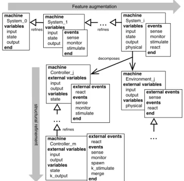
We present a stepwise and systematic method (namedHeñcher) to construct critical em-bedded control systems using Event-B. We reuse the approach already established and demonstrated in several case studies [2,3,4], following which complex systems can be constructed by combining 1) horizontal refinement with feature augmentation where we have to build a global abstract model of a the whole system (a controller and its physi-cal environment) (Sect. 2.1) and 2) structural refinement (making the abstract structures more and more concrete (Sect. 2.2). But we extend it and provide dedicated guidelines at different steps, which help the developers to reach quickly a correct control system. Fig. 1 illustrates the Event-B patterns from the most abstract model which describes only the interface of the controller, to the systematic decomposition into two parts: the

Controllerand the physicalEnvironment.

refines Feature augmentation machine System_0 variables input state output end machine System_i variables input state output physical events sense monitor stimulate react end decomposes machine Environment_j external variables input output variables physical external events sense events react end machine Controller_j external variables input output variables state external events react events sense monitor stimulate end machine Controller_m external variables input output variables state k_output external events react events sense monitor spawn k_stimulate merge end st ru ct u ra l re fin e me n t

...

...

...

Fig. 1. Synoptic structure of the Event-B models of the construction

2.1 Horizontal Process: Building an Abstract Global Model of the System The high level state space of any control system can be described by the elicitation of the interface variables between the digital part (the controller) and the physical part (the controlled environment) of the considered system.

Step 1: Characterise the abstract model of a considered system input Controller Controlled environment physical state output aact sense aact react state aact stimulate aact monitor

Fig. 2. A generic shape for event-based model of a control system

Fig. 2 depicts a general principle that may govern the organisation of event-based models of control systems. The dashed ovals are representative of the parametric events families; They should be replaced by the effective events related to the logic of a specific case study. Besides, the identi-fied physical devices to be

con-trolled should be precisely listed. The behaviour of each one will be specified later. Step 1.1: Elicit the interface We distinguish in our method, a first step which consists in the description of the interface variables of the controller. There are three categories of variables at the interface of a controller with the controlled environment.

– the input variables: they give the sensed state of the environment (the value given by sensors); they are read by the controller;

– the state variables: they are set and modified by the controller; they are used for monitoring the whole system;

– the order output variables: they are those used to send the orders that stimulate the physical environment; their values will be used by actuators.

These categories of variables will be used at different levels of the modelling and re-finement of the system at hand: to introduce the events of the first abstract model and, for refining gradually the first model. Additionally, we have the category of internal variables, which are only used inside the controller.

Step 1.2: Elicit the global properties of the system The required system properties, in-cluding safety, liveness and non-functional properties should be explicitly named and listed in their informal form. These properties will be formalised and gradually intro-duced with their formal form during the various construction steps of our method. Step 1.3: Start with a first abstract model Use the interface variables resulting from Step 1.1 to build a first Event-B abstract model. This abstract model comprises in the related B machine clauses, the interface variables together with the appropriate abstract sets and properties which characterise them. This Event-B model will be enriched to obtain a global abstract model of the system including its control part, its physical part and their related properties. Global properties of the system (among those already listed in Step 1.2) should be formalised and introduced according to the available variables. Notice that the enrichment incorporates gradually the details of the physical environ-ment (sensors and actuators) and the corresponding properties.

Step 1.4: List the events of the abstract model The Event-B abstract model resulting from the previous step will be enriched with a series of events built by defining a family of events related to each category of the interface variables: sense events, monitor events and stimulate events.

– Sense events family This family gathers the events used to set and to modify the values of the inputvariables. For each variable of this category, define an event named after the variable, with the prefix sense_. The link with the physical (state variables of the) environment is done later by refining these events in Step 2.2.

– Monitor events family These events modify the appropriate state variables. For each vari-able of this category, define an event named after the varivari-able with the prefix monitor_, to set the variable according to the current state of the controller and the input data.

– Stimulate events family The events of this family modify the order output variables; each variable of this category is set with an event named after the variable with the prefix stmlt_. These events use the internal variables, the input variables and the output variables. Associ-ated with these events to stimulate the physical devices, we may have as many events to stop the stimulation of the devices; accordingly these events have their name prefixed withstop_.

These three families of events, together with the reaction events family introduced later, are compliant with the standardsense-decision-controlof the control cycle. Step 2: Extend the abstract global model

Use feature augmentation [2,3,4] to integrate the controlled environment. This is pre-cisely achieved on the basis of the sense events family, which in turn need the descrip-tion of the controlled environment. The global properties listed before are also gradually formalised in the model, as invariants, as soon as the appropriate variables are available. Two sub-steps are distinguished but no matter their order during the development. Step 2.1: Introduce the physical environment and the reaction events family It con-sists in adding successively to the model, events to propagate the values of interface output variables inside the physical environment. These events simulate or stop the behaviours of physical devices via the actuators. The feature augmentation is used to introduce the physical state variables, invariants and appropriate behaviours. Depend-ing on the cases, either one simulates the behaviour of the physical devices with an abstract model, or the values of the output variables (from the interface) result in sig-nals sent to the environment. In this last case we do not have dedicated events in the abstract model. Accordingly, the behaviours of the physical devices should be formally described. These behaviours, systematically guarded by the values of the output vari-ables, may impact the state of the environment and finally they may impact the sensors. State automata can often be used to capture the behaviour of a physical device; describ-ing the automata with B events is then straightforward. The description of the physical part behaviour results in the family of reaction events. These events should be named using as prefix the identifier of the physical part that they describe.

Step 2.2: Detail the sense events family Each event of the sense family, updates an input variable according to the state of the sensors; for this purpose the event needs the model and the behaviour of its related sensor. Therefore the feature augmentation consists in introducing the model of the sensors and their related behaviour, as variables, invariants and related events. The behaviour of the sensors should consider the possible failures (anomalies, malfunctioning or physical defects); specific events should be described for each such possible failure.

Practically during all the refinement steps, it is recommended to proceed incremen-tally with several small refinement steps dedicated to variables and events. This is nec-essary to master the proof complexity.

Step 3: Introduce the specific properties

According to the system one has to build, besides the global properties gradually in-troduced with the variables, additional specific properties should be integrated at the abstract level to constrain the functioning of the system.

1. Reachability property with partial ordering: specific events (not at the same gran-ularity with the Event-B events) with timestamps may be systematically used to order and to reason on reachability properties.

2. Non functional properties: specific properties related to nonfunctional requirements should be gradually introduced here. No matter the way they are described, pro-vided that the mathematical support of Event-B is very large, and that external modules may be used to analyse them.

2.2 Vertical Process: Building the Concrete Parts of the System

The aim of this second process is to build the digital part and possibly the physical part of the system. The global Event-B abstract model resulting from the horizontal process should then be decomposed into various parts leading to specific components. At least we have a decomposition into a control software and a physical part. The decomposition can be performed as soon as one want to go into the details of one of the specific part by considering that the other part will stay as it is; that means no modification of the other part cannot be considered when we are refining a given one. Typically, from a decomposition step, the digital part will be refined until code by considering the events and variables of the physical part as they was at the decomposition step.

Step 4: Refine the global abstract model

We recommend to perform structural refinements as needed by the specific model to be refined. New internal B events may be added to refine the events of each family of events (sense, monitor, or stimulate). The state space variables of the global abstract model may be refined with more details in the invariant. At the end of this step, be sure that, the events of both parts are all in place, that the global required properties of the system are all in place (they cannot be introduced later after the decomposition).

Like with other formal models, an Event-B model can be animated, i.e. when appro-priate values are provided for the variables in the model, its behaviour can be observed step by step according to the semantics of the model. Animation capabilities are helpful during all the refinement steps where we still have all the events of the global system together; it will not be possible to animate the whole system after its decomposition. Step 5: Decompose into software and physical parts

A decomposition paradigm is already supported by the Event-B method. It consists in splitting a given machine into several ones which will be refined independently. The de-composition splits the variables of the state space and/or the behaviour of the machine; however resulting machines cannot contradict each other by modifying the variables and their related properties once they have been separated. Two approaches exist for this

purpose: the Abrial’style decomposition (called the A-style decomposition) [5] based on shared variables, and the Butler’style decomposition (called the B-style decomposi-tion) [6,7] based on shared events. In the A-style decomposition, events are first split between Event-B sub-components and then shared variables of the sub-components are used to introduce external events in the sub-components; these external events should be refined in the same way. In the B-style decomposition, variables are first partitioned between the sub-components and then shared events (which use the variables of both sub-components) are split between the sub-components according to the used variables. We adopt the A-style decomposition which is more relevant when considering a list of specific events to be split relatively to a control part and a physical part. The methodological guide to achieve the decomposition is as follows: the digital part is made with all the events defined in the sense events, the monitor events and the stimulate eventsfamilies whereas the physical environment gathers all the events defined in the reaction eventsfamilies. Moreover, each part must have an abstract view of the other through external variables and events.

Step 6: Refine the control software and the physical environment separately Step 6.1: Refining the control software Use Structural refinements based on the stimu-lateevents family to refine the controller. The involved categories of variables are the inputvariables, the state variables and the output variables. Typically, the values of the outputvariables are synthesised from the other ones. This can be done through simple control functions or through sub-modules.

aact k_stimulate Module 1 input Controller . . . output aact spawn aact merge k_ output[1] k_input [1] k_ output[n] k_input [n] aact k_stimulate Module n

Fig. 3. Modules redundancy When there are sub-modules, the input variables

may be spawned inside the sub-modules; in the same way output variables may be updated by promotion from the sub-modules if any. Therefore one have to incorporate successively in the Event-B model the events to set and modify the output variables; they de-scribe the result of the behaviour of the control part. State automata help to catch these behaviours; then the events of the B models encode the automata. We give now some recurrent patterns to help in modelling control part.

i). Composition of several redundant sub-modules: when a controller is made of sev-eral redundant modules, it is straightforward to describe a generic module and use an indexing function to compose several instances of such modules (see Fig. 3).

– Encasing variables inside modules: the values coming from outside one or sev-eral modules can be systematically encased inside the modules with a dedicated event that spawn the events.

– Promoting variables outside a module: in a symmetric way, the values going outside a module or several modules can be systematically described using a promotion pattern (with a dedicated event) for merging the output variables of the internal computing modules.

ii). When the modules are not redundant, each one should be refined separately, but the treatment we have described for the inputs and outputs variables is the same.

Step 6.2: Refining the controlled (physical) environment Many cases can be considered depending on the system to be studied; either the physical devices are already available, or one has to build the physical devices from the formal models, or one has to build a part of the physical devices. Nevertheless, the exchange of signal with actuators is the standard way to act on physical devices.

i). In the case where the physical devices are available, with the related actuators, the refinement is straightforward; it consists for the events of the physical part to output the correct signal values (for example on/off values are encoded as voltage) as input of the actuators. But the physical devices may be emulated in preliminary studies before implementing the control part on the real devices. Mathematical models and dedicated system engineering tools are available as explained hereafter.

ii). When the output variables of the controller cannot be immediately encoded as sig-nal values, transformation can be achieved via appropriate mathematical functions and models. This should be done, starting from the requirements and the proper-ties of the previous model, for example by external modules or functions written with tools like Matlab or Simulink1or SciLab2; related works can be found in [8]. These tools generate executable codes dedicated to the target devices. They are also equipped with specific functions to handle time requirements.

3

A Running Case Study

The proposed method is applied on the Landing Gear (LG) case study, a benchmarking example proposed at the ABZ’2014 conference to compare different formal methods in terms of expressivity, performance, and ease of use. A prerequisite for reading this section is the detailed specification of this critical embedded system given in [9]. A summary of the LG system is depicted in Fig. 4.

Mechanical and hydraulic parts

doors gears up/down Pilot interface actuators sensors Digital Part sensors

actuators front gear box

right gear box left gear box

Fig. 4. Global architecture of the LG system

The LG system is in charge of manoeuvring 3 landing boxes: front, left and right. Each landing box contains a landing gear, an as-sociated door and the correspond-ing hydraulic cylinders in charge to move gears and doors. The sys-tem is made of a controller (the digital part) and the controlled physical environment (i.e. the 3 landing gear boxes and a pilot in-terface) which interact via sensors and actuators; the sensors provide to the digital part the information on the state of its physical part; the actuators engage the orders of the controller on the physical part. The physical devices already exist, we will not build them; the challenge deals with the digital control part only (see page 2 of [9]).

1_{http://uk.mathworks.com/products/control/} 2_{http://www.scilab.org}

3.1 Horizontal Process: Building an Abstract Global Model of the System We give the main elements resulting from the successive application of the steps pro-posed in the method (Sect. 2).

Step 1.1: Elicitation and modelling of the interface variables The requirement doc-ument listed several triplicated input variables: handle, analogical switch, gear states, doors, · · ·. We model (Step 1.3) them with a type T RIPLE = {1, 2, 3} used as an index of the function variables:

GEAR = {FG, LG, RG} analogical_switch ∈ T RIPLE → AnalSW STAT E DOOR = {FD, RD, LD} handle∈ T RIPLE → HSTAT E

HSTAT E = {hDown, hU p} gear_extended ∈ (T RIPLE × GEAR) → BOOL AnalSW STAT E= {openSW, closedSW } door_closed ∈ (T RIPLE × DOOR) → BOOL

· · · ·

The function variable handle ∈ T RIPLE → HSTAT E captures precisely the re-quirement handlei∈ {hDown, hU p} with i ∈ {1, 2, 3}. The state variables are the states of the gears, doors, anomalies, etc. They are modelled as follows:

gears_locked_down ∈ BOOL ∧ gears_maneuvering ∈ BOOL ∧ anomaly ∈ BOOL ∧ · · ·

The output variables hold the values computed for various electro-valves:

general_EV ∈ BOOL ∧ close_EV ∈ BOOL ∧ open_EV ∈ BOOL ∧ · · ·

The lights which indicate the position of the gears and doors to the pilot are des-cribed as internal variables: greenLight, orangeLight, redLight. These variables are bound to the output state variable gears_locked_down with an invariant predicate. An-other internal variable order is used to record the action of the pilot on the handle.

The LG system is controlled digitally in the normal mode until an anomaly is de-tected. A permanent failure leads to an emergency mode where the system is controlled analogically. Accordingly the internal boolean variable anomaly is used to denote that an anomaly has been detected or not.

Step 1.2: Elicitation of the global properties of the LG system Most of the normal mode requirements are safety properties. Some identified ones are the following:

R21We can not observe a retraction sequence (consequence of the order hU p) if the handle

is down. Using the enumerated set HSTAT E which permits only one value from two for the variable order.

R31The gears outgoing event occurs if doors are open locked.

R41Opening and closing doors electro-valve are not stimulated simultaneously.

R51It is not possible to stimulate the manoeuvring EV (opening, closure, outgoing or

re-traction) without stimulating the general EV.

The first Event-B abstract model resulting from Step 1.3, gathers all the variables of the interface, their related invariants and initialisations. Event-B contexts are used to model the static part with the various sets and definitions that we have introduced.

Step 1.4: The families of events of the abstract model A thorough analysis of the two action sequences (outgoing sequence and retraction sequence) described in the LG sys-tem helps us to capture the behaviour of the digital part and to derive the events. We use here state automata to make it clear the interaction between the different components (actions of the pilot, the controller, the orders received by the environment).

In the sense event family we have listed for example the eventsense_gearto modify the input variable gear_extended listed above. In the same way we have listed the other eventssense_door, etc. Examples of events we have identified for the control events family are:stmlt_general_EVto stimulate the general electro valve,stmlt_door_opening,

stmlt_gear_outgoing,stop_stmlt_general_EV,stop_ stmlt_gear_outgoing, etc.

Each one modifies its related variable, for instance the eventstop_stmlt_gear_outgoing

sets the variable extend_EV to FALSE. Examples of event we have classified in the monitor eventsfamily are: monitor_ anomaly, monitor_gears_locked_Down, monitor_ gears_maneuvering.

Step 2: Extension of the abstract global model with the event families We achieve many refinement steps, by feature augmentation, to integrate gradually the variables and events related to the physical devices: the sensors, the doors and the gears.

Following Step 2.1, we define the behaviours of physical devices. For instance, the door behaviour is first captured with a state automata; the transitions of the automata are then described as events. For this purpose we use a transition function doorState ∈

DOOR→ DSTAT E where DSTAT E = {ClosedLocked,ClosedUnlocked,

OpenUnloc-ked} is the enumerated set of the identified door states. The set DOOR contains the three door identifiers. The function doorState is a total function; this captures the requirement that all the three doors are controlled via the state transition.

The starting transition of the door behaviour is enabled by the open_EV order given by the digital part. Therefore there is a synchronisation between the digital part and the motion of the doors. We only give below the description of the starting event

Door_openDoor_cl2cu; the other necessary events are similar.

eventDoor_openDoor_cl2cu

/* Door’s Behaviour (for the three doors). The first transition of the Door Automata */ where

@g1 open_EV = T RU E // all the doors Electro Valves are on @g2 ran(doorState) = {notOpenLocked}

then

@a1 doorState := DOOR × {notOpenNotLocked} // door is being opened end

The following event describes an event of the control event family.

eventstmlt_gear_outgoing

/* stimulate gear outgoing electro valve once the three doors are in the open position */ where

@g0 general_EV = T RU E @g1 order = hDown @g2 ran(handle) = {hDown}

@g4 ran(door_open) = {T RU E} @next nextOGseq = 3

@gano anomaly = FALSE // no anomaly detected @notretract retract_EV = FALSE

then

@a1 extend_EV := T RU E

@a2 nextOGseq := nextOGseq + sequenceStep end

The variable nextOGseq controls the evolution of the outgoing sequence; it indicates in the event guards, the next step in the outgoing sequence. We note that the events in the sense event family anticipate their real future specifications, which are related to the physical part introduced later. When we have introduced the various events families and the related variables, it becomes clear for us that we have the complete control loop.

Following Step 2 the properties (listed in Step 1.2 above) are formalised as first order predicates, integrated into the invariant of the abstract model and, proved along the horizontal refinement. As an example, the requirement R51is described as follows.

((open_EV = T RU E ∨ close_EV = T RU E ∨ extend_EV = T RU E ∨ retract_EV = T RU E) ⇒ general_EV = T RUE)

To sum up, the global Event-B abstract model results from a series of refinement of contexts and machines.

Step 3: Dealing with specific properties In this case study, reachability is one of the specific properties. Based on the idea of Lamport’s logical clocks [10], we implement a technique that captures the reachability requirement R1given in page 13 of [9]. For that purpose, we introduce the notion of control cycle, a period of time during which one can observe several events, especially a chain of events denoting an outgoing sequence or a retraction sequence; a typical control cycle is one starting with an event (downH) which denotes the hDown order and terminating by an event (dcge) which denotes the fact that “the gears are locked down and the doors are seen closed”; similarly, another control cycle is started when the handle triggers an order hU p. A dedicated variable endCycleis used to control the start and the end of each control cycle.

Given a set obsEvents of events (for instance the starting of an outgoing sequence, a door closed, a gear locked in a position, etc.) and a logical clock modelled as a natural number, the occurrences of the events can be ordered by the timestamps given by the clock. In our case two events cannot happen at the same time. We use a partial function ldate∈ obsEvents 7→ N to record the timestamps of the events. We can compare and reason on the timestamps of any events happening during a sequence and specifically within the specific event sequence called control cycle. An example is as follows.

∀d j.(((d j ∈ N) ∧ (dcge ∈ dom(ldate)) ∧ (d j = ldate(dcge)) ∧(endCycle = T RUE) ∧ d j < llc) ⇒

∃di.((di ∈ N) ∧ (downH ∈ dom(ldate)) ∧ (di = ldate(downH)) ∧ (di < d j)∧ ∀ii.(ii ∈ N ∧ di ≤ ii ∧ ii < d j ⇒ ldate ∼ [{ii}] 6= {upH})))

To put into practice in Event-B withRodin, we defined the set obsEvents in the context of our machines, and the above property is included in the invariants of the abstract model.

3.2 Vertical Process: Building the Concrete Parts of the LG System

The vertical process includes several refinements (in Step 4) described below follow-ing the proposed method. We end our process with the Step 5. The Step 6 was not performed for the LG case study because only the digital part will be refined with the objective to build the software part. The variables and events which are specific to the behaviour of the physical part are not refined but we keep them in the model in order to preserve animation capabilities. This approach is very pragmatic.

Step 4: Structural refinements of the global abstract model The requirement docu-ment details the inner structure of the digital part; it is made of two redundant com-puting modules. We achieve structural refinement steps to overcome the details of the behaviour of the digital part.

a) Introducing the two computing modules with refinements Both modules have the same interface (input and output variables) inherited from the abstract model of the digi-tal part. Each interface variable of a module k (where k ∈ {1, 2}) is inherited from a vari-able (for instance gear_extended) of the digital part of the abstract model and it is de-noted by k_gear_extended(k) where k is an index. An enumerated set CompModule = {1, 2} is used for the indexes. Therefore each interface variable of the computing mod-ules is specified with the following shape:

k_gear_extended ∈ CompModule → ((T RIPLE × GEAR) → BOOL) The binding between the two modules interface variables and those of the abstract mod-ule is achieved via refinements where new variables and related events are introduced. b) Spawning the inputs inside the computing modules with refinements We introduced new events (prefixed with spawn_) to push the value of each input variable (for example handle) at the abstract level, in the corresponding variable (for example k_handle) of each computing module. As the inputs of the modules should be the same, an invariant is defined in each case of variable spawning in order to guarantee the correctness of the binding between the input variable of the digital part and the same input of the computing modules. The following event pattern spawns the variables at the interfaces of the computing modules.

eventspawn_handleDown // spawn handleDown within the k CompModules where@g1 ran(handle) = {hDown}

then

@a1 k_handle := {1 7→ (T RIPLE × (ran(handle))), 2 7→ (T RIPLE × (ran(handle)))} end

We have identified a reusable specification rule: a new event is introduced along with each new k-indexed variable. This event should copy the variable at high level (the digital part) into the indexed variables at the low level. Furthermore, the existing events, whose guards or actions involve the spawned variables, should be refined by extending their guards and actions in order to satisfy the binding between the variables and the associated k-indexed variables. One noticeable feature in this case is that when we have a non-deterministic event of abstract level (as for the value of the sensors), then in the refinement the event should be refined (not extended). This is another reusable specification rule we have identified.

c) Merging the outputs of the computing modules with refinements As depicted in Fig. 3, the k-indexed output variables (for example k_extend_EV (1) and k_extend_EV (2)) are merged using a logical OR to set the corresponding variable (for example extend_EV ) at the output of the digital part. Therefore the event that sets the variable should be guarded by the availability of the merged value. As explained before, a binding invariant should be provided for each variable and the related k-indexed variable. Several refinements are used to introduce the appropriate events.

d) Specifying the behaviour of the computing modules The two computing modules have the same behaviour. It is made of the events that monitor the system and set ac-cordingly the state output variables and the input variables of the digital part, the events that give orders (control decision) to the physical part through the order output vari-ables. It results in the k-indexed form of the events related to the three categories of the interface variables and the internal variables.

We stopped our construction at this stage. However following the guidelines pro-vided in the method, it remains to perform the decomposition step in the basis of the sense, monitor, control events families (Step 6).

4

Assessment and Discussion

Coverage Applying the proposed method helped us a lot in mastering the case study. The resulting Event-B model presented in this article covers the main aspects of the landing system: the digital part with modules redundancy, its physical part and their interactions. The model covers mainly the safety properties of the LG system; liveness properties are treated by adapting Lamport’s logical clocks [10]; but we have not deal with time constraints. Code generation was out of the scope of the current work. Never-theless the management of huge B models is still tedious, since modifying the models already equipped with a lot of variables an events, at more abstract level requires redo-ing several steps of modellredo-ing, refinements and provredo-ing.

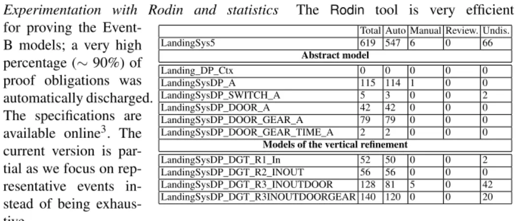
Experimentation with Rodin and statistics The Rodin tool is very efficient

Total Auto Manual Review. Undis.

LandingSys5 619 547 6 0 66 Abstract model Landing_DP_Ctx 0 0 0 0 0 LandingSysDP_A 115 114 1 0 0 LandingSysDP_SWITCH_A 5 3 0 0 2 LandingSysDP_DOOR_A 42 42 0 0 0 LandingSysDP_DOOR_GEAR_A 79 79 0 0 0 LandingSysDP_DOOR_GEAR_TIME_A 2 2 0 0 0

Models of the vertical refinement

LandingSysDP_DGT_R1_In 52 50 0 0 2

LandingSysDP_DGT_R2_INOUT 56 56 0 0 0

LandingSysDP_DGT_R3_INOUTDOOR 128 81 5 0 42

LandingSysDP_DGT_R3INOUTDOORGEAR 140 120 0 0 20

Table 1. Statistics of PO generated and proved withRodin

for proving the Event-B models; a very high percentage (∼ 90%) of proof obligations was automatically discharged. The specifications are available online3. The current version is par-tial as we focus on rep-resentative events in-stead of being exhaus-tive.

Statistics on Proof Obligations are given in Tab. 1. From a total of 619 POs, 547 of them were automatically discharged byRodinand 6 of them were interactively dis-charged. Most of the POs at the abstract levels were proved. The undischarged POs are related to the structural refinement and specifically they are related to the binding invariants.

Managing very large models requires a rigorous slicing and several small steps of refinements. This is the reason why we have introduced many refinements, but it is still not enough, the slicing should be of finer grain. Moreover a good naming discipline is necessary at each level of the modelling. As far as the ProB animation tool (integrated inRodin) is concerned, it is very helpful to tune the Event-B models.

Related Works The state of the art lacks of assistance methods. The four-variable model of software-controlled embedded systems originally proposed by Parnas and Madey has been used successfully in the development of safety-critical applications in various industries. But as mentioned by [11], the model does not explicitly specify the software requirements, but rather bounds them by specifying the system requirements and the input and output hardware interfaces of the system.

We share the same the motivations with [12]. However the authors propose a method to synthesise the controller from the environment behaviour. Indeed they introduced the controller and its interface as a solution to the problem of maintaining a desired behaviour of an autonomous system. In our approach the controller is not synthesised to maintain a specific behaviour; it is built simultaneously with the environment according to the given control requirements, but the environment behaviour is less constrained by the controller.

As far as method is concerned in the treatment of the LG system benchmark, all the related B specifications of the LG System are based on refinements. They do not de-scribe a precise methodological process. Often, the authors need about ten refinements to include properties and requirements. The distinction between them is rather the way the refinements are organised rather than on methodological assumptions.

Su and Abrial [13] mentioned that there is no definitive answer for applying some recipe since the question vary from one project to another. They propose a light method-ology including three steps: informal requirements, refinement strategy and formal model. They excluded features like redundancy and simplified time constraints. The systematic refinement strategy integrates progressively the devices, which is rather spe-cific to the case study. Accordingly, our method focuses on a more general refinement strategy.

Mammar and Laleau adopted the four-variable model of software-controlled em-bedded systems originally proposed by Parnas and Madey. They used a series of refine-ments [14] first according to a variable classification first (monitor, control, output) then including timing aspects, failure cases and last properties. Mammar and Laleau focused on the control part only. Since it appears to be a logical organisation, a separation of concerns, this ordering delays most of the proof work to the last refinements. It lost modularity and extensibility.

R. Banach used Hybrid Event-B to lead his study [15]; this extension enables one to carry continuous varying behaviours. R. Banach proposed a proof of concept of the

language extension rather than a method or a full answer to the case study. However, hybrid-B seems adequate to refine the physical part of our current specification and especially to model time requirements.

Hansen et al. focused on the validation of the case using ProB rather than on the methodology of specifying with B [16]. As a matter of fact, the temporal properties are naturally introduced using LTL expressions. Another interesting feature is the abil-ity to visualise the system execution. The counterpart is a simplified specification (no redundancy, no physical part, no failure). The refinements start with physical devices (door, gears, electro-valves), then the output, sensor and controllers are introduced as refinements and finally the general control (switch, valves, lights).

5

Conclusion

We proposed a method (namedHeñcher) to guide step by step the construction of em-bedded control systems with Event-B. We build on the well-known structure of control systems and on the experiments of several case studies where the Event-B was used and where some methodological guidelines was provided [3,2]. We provide a system-atic use of the interface of the controller to build the components of the abstract model of the control system and, also how the features of the control system should be used to guide the successive refinements of the abstract model. A non trivial case study served as illustration and assessment of the proposal.

One flaw of the Event-B top-down approach is the constraint imposed by the evolu-tion of the global abstract model defined before its refinement to the concrete models. This constraint prevents for an incremental model evolution. Indeed, if we miss some features in the abstract state, we will have to reconsider completely the structural refine-ments. It would be interesting to be able to mix both horizontal and vertical refinements in an incremental view of the design method. In [17] Back, have proposed guidelines for this purpose; an adaptation of this work to Event-B is likely to be interesting.

The reuse of existing independent models, with a bottom-up approach, would be interesting for managing large Event-B models. A typical example is the composition of existing models to build a given abstract model where each part can be modified and refined separately.

We plan to develop an assistance tool to help the user with various patterns, in the form of Event-B machines derived from the interface variables which will be extracted from a sketched graphical view of its control system (as in Fig. 2).

References

1. Jard, C., Roux, O.H., eds.: Communicating Embedded Systems: Software and Design. Wiley-ISTE (2009)

2. Damchoom, K., Butler, M.J.: Applying Event and Machine Decomposition to a Flash-Based Filestore in Event-B. In: 12th Brazilian Symposium on Formal Methods, SBMF 2009. Vol-ume 5902 of LNCS., Springer (2009) 134–152

3. Damchoom, K., Butler, M.J., Abrial, J.R.: Modelling and Proof of a Tree-Structured File System in Event-B and Rodin. In: 10th International Conference on Formal Engineering Methods, ICFEM 2008. Volume 5256 of LNCS., Springer (2008) 25–44

4. Abrial, J.R.: Modeling in Event-B - System and Software Engineering. Cambridge Univer-sity Press (2010)

5. Abrial, J.R., Hallerstede, S.: Refinement, Decomposition, and Instantiation of Discrete Mod-els: Application to Event-B. Fundam. Inform. 77(1-2) (2007) 1–28

6. Butler, M.: Decomposition Structures for Event-B. In: 7th International Conference on Integrated Formal Methods, IFM 2009. Volume 5423 of LNCS., Springer (2009) 20–38 7. Silva, R., Butler, M.: Shared Event Composition/Decomposition in Event-B. In: 9th

Inter-national Symposium onFormal Methods for Components and Objects, FMCO 2010. Volume 6957 of LNCS., Springer (2012) 122–141

8. Su, W., Abrial, J.R., Zhu, H.: Complementary Methodologies for Developing Hybrid Sys-tems with Event-B. In Aoki, T., Taguchi, K., eds.: Formal Methods and Software Engineer-ing. Volume 7635 of LNCS., Springer Berlin Heidelberg (2012) 230–248

9. Boniol, F., Wiels, V.: The landing gear system case study. [18] 1–18

10. Lamport, L.: Time, Clocks, and the Ordering of Events in a Distributed System. Commun. ACM 21(7) (1978) 558–565

11. Patcas, L.M., Lawford, M., Maibaum, T.: From system requirements to software require-ments in the four-variable model. ECEASST 66 (2013)

12. Hudon, S., Hoang, T.S.: Development of Control Systems Guided by Models of Their Envi-ronment. Electron. Notes Theor. Comput. Sci. 280 (December 2011) 57–68

13. Su, W., Abrial, J.R.: Aircraft landing gear system: Approaches with event-b to the modeling of an industrial system. [18] 19–35

14. Mammar, A., Laleau, R.: Modeling a landing gear system in event-b. [18] 80–94 15. Banach, R.: The landing gear case study in hybrid event-b. [18] 126–141

16. Hansen, D., Ladenberger, L., Wiegard, H., Bendisposto, J., Leuschel, M.: Validation of the abz landing gear system using prob. [18] 66–79

17. Back, R.J.: Software Construction by Stepwise Feature Introduction. In: 2nd International Conference of B and Z Users. Volume 2272 of LNCS., Springer (2002) 162–183

18. Boniol, F., Wiels, V., Ait Ameur, Y., Schewe, K.D., eds.: ABZ 2014: The Landing Gear Case Study. In Boniol, F., Wiels, V., Ait Ameur, Y., Schewe, K.D., eds.: ABZ2014. Volume 433 of CCIS., Springer International Publishing (2014)