HAL Id: hal-01666698
https://hal.archives-ouvertes.fr/hal-01666698
Submitted on 6 Nov 2019
HAL is a multi-disciplinary open access archive for the deposit and dissemination of sci-entific research documents, whether they are pub-lished or not. The documents may come from teaching and research institutions in France or abroad, or from public or private research centers.
L’archive ouverte pluridisciplinaire HAL, est destinée au dépôt et à la diffusion de documents scientifiques de niveau recherche, publiés ou non, émanant des établissements d’enseignement et de recherche français ou étrangers, des laboratoires publics ou privés.
An estimation of stress intensity factor in a clamped
SE(T) specimen through numerical simulation and
experimental verification: case of FCGR of AISI H11
tool steel
Masood Shah, Catherine Mabru, Farhad Rezai-Aria, Inès Souki, Riffat Asim
Pasha
To cite this version:
Masood Shah, Catherine Mabru, Farhad Rezai-Aria, Inès Souki, Riffat Asim Pasha. An estimation of stress intensity factor in a clamped SE(T) specimen through numerical simulation and experimental verification: case of FCGR of AISI H11 tool steel. ACTA METALLURGICA SINICA-ENGLISH LETTERS, 2012, 25 (4), pp.307-319. �10.11890/1006-7191-124-307�. �hal-01666698�
An estimation of stress intensity factor in a clamped SE(T)
specimen through numerical simulation and experimental
verification: case of FCGR of AISI H11 tool steel
Masood Shah 1)§, Catherine Mabru 2), Farhad Rezai-Aria 3), Ines Souki 3)
and RiÆat Asim Pasha 1)
1) Mechanical Engineering Department, University of Engineering and Technology, Taxila, Pakistan 2) Department of Mechanics of Structures and Materials, University of Toulouse; INSA, UPS, Mines Albi,
ISA; ICA (Institute Cl´ement Ader); DMSM, F-31056 Toulouse, France
3) Research Group of Surfaces, Machining, Materials and Tooling, University of Toulouse; INSA, UPS, Mines Albi, ISAE; ICA (Institute Cl´ement Ader); Campus Jarlard, F-81013 Albi cedex 09, France
A finite element analysis of stress intensity factors (KI) in clamped SE(T)Cspecimens
(dog bone profile) is presented. A J-integral approach is used to calculate the values of stress intensity factors valid for 0.125∑a/W ∑0.625. A detailed comparison is made with the work of other researchers on rectangular specimens. DiÆerent boundary conditions are explored to best describe the real conditions in the laboratory. A sensitivity study is also presented to explore the eÆects of variation in specimen position in the grips of the testing machine. Finally the numerically calculated SIF is used to determine an FCGR curve for AISI H11 tool steel on SE(T)C specimens
and compared with C(T) specimen of the same material.
KEY WORDS Fatigue crack propagation; Stress intensity factor; J–Integral; Paris law
NOMENCLATURE SE(T) Side edge cracked, tension specimen
SE(T)C Side edge cracked, clamped tension specimen
a/W Crack length to specimen width ratio C(T) Compact tension specimen
a Crack length B Specimen thickness
W Specimen width inside gauge length We Specimen width at the specimen ends
H Specimen height
H/W Height to width ratio of specimen s Length of the arc around the contour y Direction perpendicular to crack plane
v, u Displacement parallel to y axis and x axis, respectively ¿§ Displacement vector
w Strain energy density
§Corresponding author. Assistant Professor, PhD; Tel: +92 51 90472297, Fax: +92 51 9047690.
° Contour for J-Integral T Traction vector
F Force perpendicular to crack plane K Stress intensity factor
KI Mode I stress intensity factor
E Young0s modulus
FEA Finite element analysis " Strain
r Distance from the crack tip æy Yield stress
∫ Poisson0s ratio
Uy Displacement applied at the end of a specimen
Rx, Ry, Rz Rotation of specimen ends along x, y and z axis respectively
f Reaction force on each node of an finite element model f (a/W ) Geometric correction factor for stress intensity factor ¡ Ratio of in plane rigidity of gauge length
to in plane rigidity of specimen ends FCGR Fatigue crack growth rate
1 Introduction
To test the surface damage of die steels, small specimen of very low thickness is needed[1,2]. This is due to the fact that the surface damage in tool steels may extend
from 50–300 µm below the loaded surface and the tested specimen should be of the order of this size. For this purpose clamped SE(T)Cspecimens provide a good alternative to C(T)
specimens because they completely remove the possibility of buckling or bending during tensile fatigue testing. The same problems of buckling and bending would be present in pin loaded specimens (eÆects of non symmetric rotation) as well as failure in the bearing surfaces since the specimen thicknesses can be as low as 0.10 mm[1,2]. Also the free standing
surface keeps a flat view towards the camera throughout the test which is very important for making small measurement of the order of 10 µm accurately. In addition, standard ASTM specimens would be di±cult to machine in the dimensions imposed by the testing conditions we are trying to copy. A
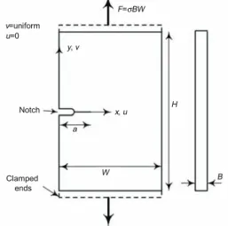
schematic for the single edge cracked speci-men is shown in Fig. 1, where B is thickness, a is crack length, W is specimen width, H is height. The direction of the applied load is also shown. However, a method is needed to calculate accurately the stress intensity fac-tors generated in these specimens.
Indeed, KI is known to be dependent
on the H/W ratio and the end condi-tions as shown in literature[3°5]. It is also
observed that in practice the position of the specimens inside the grips may vary slightly from one experiment to another. The influence of these variations on the KI values needs to be assessed to
deter-mine its eÆects on the interpretation of the
Fig. 1 Schematic of the single edge cracked tensile specimen with clamped ends, SE(T)C
results of the experiments. Numerous studies addressing the numerical calculations of SIF are reported in the literature. One of the most common methods relies on the extrapolation of displacements in the vicinity of the crack tip[6,7]. The other method is based on an
energetic approach and consists of determining the J-integral values or the equivalent domain integral[3,4,6].
In this paper the finite element simulations are carried out in ABAQUS/StandardTM
software package. The software has the possibility of giving direct K output or values for J-Integral. But in both the cases the basic calculation is carried out using the J-integral approach. The J-Integral introduced by
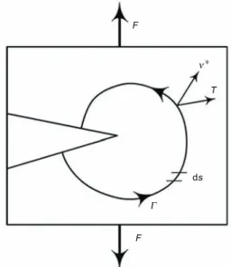
Rice[8]is shown schematically in Fig. 2. Here,
a material with a crack is monotonically loaded by a force F in the direction perpen-dicular to the direction of crack propagation. Considering T as traction independent of the crack length on a contour ° around the crack tip and assuming there is no load on the crack faces, the integral “J” around the contour ° is given by Eq. (1).
J =
Z
°
(wdy ° T@v@x§ds) (1) The elastic J-Integral calculated in this manner may be easily related to the elastic mode I stress intensity factor KI. So instead
of using the software output, KIwas directly
calculated using Eq. (2).
Fig. 2 Schematic of a cracked body loaded for contour integral or “J-Integral” calcu-lation
J = KI2/E0 (2)
where E0=E for plane stress and E0=E/(1°∫2) for plane strain.
The J-integral is independent of path where the path begins at the lower crack face and ends at the upper crack face as long as the tractions are zero on the crack faces and the crack is along the x-axis. Due to this property the numerical simulation can be carried out for fairly coarse mesh without much problems[6].
In the present paper, a J-integral approach is used to calculate KI values for clamped
SE(T)C specimens. EÆects of H/W ratio and boundary conditions on KI values are
in-vestigated and compared to literature data[3°5]. A sensitivity study is particularly carried
out to evaluate the influence of the variation of the specimen position inside the grips on the calculated KIvalues. SIF values obtained for specimens with 2.5 mm in thickness, are
applied on thinner specimens (down to 0.1 mm) as well. This was justified by the fact that we needed a single criterion to compare FCGRs of specimens of diÆerent thicknesses. The SIF thus calculated for the SE(T) specimens is used to determine the FCGR or Paris curves for a high strength tool steel, AISI H11 and the results are compared with the Paris curve determined using the C(T) specimen on the same material.
2 Finite Element Analysis 2.1 Finite element model
Detailed finite element analyses are performed on plane strain models of three types of 1-T SE(T)C specimens, all having a thickness of 2.5 mm using the software package
ABAQUS/ StandardTM. The analysis is carried out on diÆerent rectangular specimens
with height to width ratio (H/W ) of 1, 1.5, 2, 2.5 and 3 respectively, as well as on one dog bone type specimen. Only the specimens of H/W of 2, 3 and the dog bone type specimens are shown in Fig. 3.
As indicated above the KIis dependent on the H/W ratios in rectangular specimens.
This does not pose a problem as long as the test specimens are rectangular and the KI
values may be obtained directly in the literature. However, when using a dog bone spec-imen as in this paper, the situation is more complex. In this example, there are diÆerent H/W ratios; for gauge length it is 1.875 and
that for the unconstrained length between grips is 3.125. It may also be noted that in the unconstrained length between grips there are shoulders which change the compli-ance of the specimen due to variable section along the length. This specimen thus has to be considered as a structure instead of a simple rectangular specimen. However since the two extreme H/W ratios possible are be-tween about 2 and 3, the numerical analysis procedure is verified for these two H/W val-ues only by comparison with the literature.
Although the finite element analyses are carried out on all the specimens (rectangular and dog bone), the procedure is described only for the dog bone specimen whereas the procedure for other two geometries stays the same. Figure 4 shows the finite element model constructed for the SE(T)C specimen
along with the meshing. In the rectangular specimens, a is the crack size including the notch, W is the width of the specimens and H is the height. The rectangular specimens are analyzed with the intention of compar-ing the results obtained with those of other researchers[3°5]. The comparison will be
pre-sented in the results section.
All the specimens are tested for 0.125∑a/W ∑0.625 which corresponds to crack lengths of 1 mm to 5 mm in a to-tal width of 8 mm. A conventional crack
Fig. 3 Schematic of the SE(T)C specimens
used in finite element analyses: (a) rectangular H/W =2; (b) rectangular H/W = 3; (c) dog bone used in FEA and experiments (unit in mm)
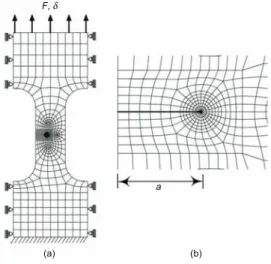
Fig. 4 Finite element model used in plane strain analyses: (a) complete specimen; (b) region of interest around the crack tip
analysis mesh configuration is used with a focused ring of 15-node quadratic tri-angular prism (C3D15) elements around the crack tip (Fig. 5). Around this first cylinder of triangular elements five con-centric rings of 20-node quadratic brick, reduced integration (C3D20R) elements are generated. These rings are subse-quently used for calculation of the J-Integral wherein the values on the first ring are ignored[9]. There has to be convergence on all
Fig. 5 Schematic of stepwise procedure of meshing
other element rings for results to be valid (see ABAQUS/StandardTM user0s manual[9] for
a detailed explanation).
The position of the center of these rings defines the crack front. A typical 3D finite element mesh contains about 10000 elements. A transverse plane surface is then chosen from the center of the rings to the crack edge which is defined as the partition or the crack plane. During the finite element analysis ABAQUS/StandardTM duplicates the nodes
on the crack plane and then assigns one set of nodes to one face and the other set to the other face. This creates a crack with no opening at the beginning, while a strain singularity at the crack tip. However since the large strain zone is very localized at the singularity the problem can be solved satisfactorily using small-strain analysis. The crack tip strain singularity depends on the choice of the material model used. In this analysis an incremental plasticity model is used. If r is the distance from the crack tip then the strain singularity is valid for small strain is Eq. (3).
"/ 1/pr (3)
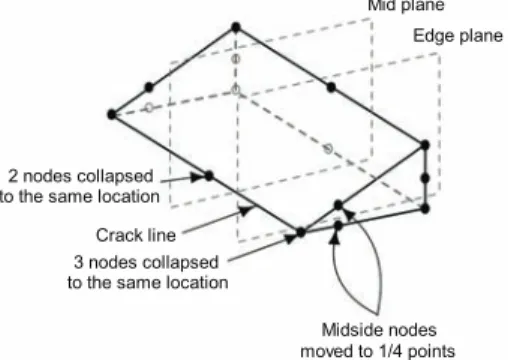
This singularity is automatically built into the finite element model in ABAQUS/Stand-ardTM with the help of the triangular prismatic elements which are used to represent
collapsed quadratic elements. The need for creating “quarter point” nodes manually is essentially eliminated. There is a quarter point element that leads to a square root stress singularity that simulates the collapsing of
quadratic into a wedge element[9]at the crack
tip (Fig. 6).
The finite element code ABAQUS/Stand-ardTM provides the numerical solutions for
plane strain analyses for 3D models as presented here. The evaluation of the J-integral is based on the domain J-integral procedure[8,9] which yields J values in
ex-cellent agreement with other methods of calculation[6]. The procedure is supposed
to maintain strong path independence for domains outside the highly strained material near the crack tip. Such J values provide
Fig. 6 C3D20R element collapsed on one side to create a singularity, the collapsed el-ement can be simulated automatically by using a C3D15 element
a convenient parameter to characterize the average intensity of far field loading on the crack front. The advantage being that we can directly calculate the KI stress intensity
factor values using Eq. (2).
The conditions described above, have also been used for the rectangular specimens. The density of the mesh around the crack tip, no of contours around the crack tip (as described in section 3.1), no of layers of elements, as well as the density of the mesh at the specimen ends, used to calculate the reaction force remains the same for the rectangular specimens and the dog bone specimens. The total number of nodes in each simulation varies, due to the fact that a constant mesh density is used.
2.2 Computational procedure
2.2.1 Material The material defined for all analyses is an incremental plasticity mate-rial using values for an X38CrMoV5 hot work tool steel with, E=206 GPa, æy=1100 MPa,
∫=0.27. The charge in all the specimens never exceeds 250 MPa in total thus giving a fairly accurate approximation to a linear elastic analysis with a confined plastic zone. Three diÆerent types of analyses have been performed which are detailed separately as follows.
2.2.2 Rectangular specimens and boundary conditions The main purpose of testing the rectangular specimens is to compare the procedure of numerical analysis explained above with that of other researchers[3°5]. The analysis has also been used to correctly
identify the eÆect of diÆerent boundary conditions for the calculation of KI; (i) with one
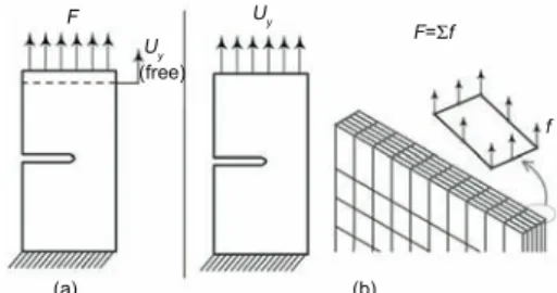
end fixed while a uniform force applied on the other end or (ii) one end fixed with a uniform displacement applied at the free end. Two diÆerent H/W values (Figs. 3a and 3b) have been used because the final dog bone (Fig. 3c) specimen falls within this ratio as discussed above. Figure 7 shows the end conditions in detail.
In the first set of boundary conditions Fig. 7a, one end of the specimen is fixed while at the other end a uniform force is ap-plied such that the total force is equal to F , while the displacement of this face is kept completely free. In the second set of bound-ary conditions (Fig. 7b), one end is fixed as before while a fixed displacement Uy is
ap-plied on the other end. The magnitude of this displacement is adjusted in such a way that the sum of reaction forces f, on all the
Fig. 7 Boundary conditions: (a) applied uni-form force; (b) applied displacement
nodes of this face should be equal to the force applied in the first case F . This second set of boundary conditions follows more closely the real testing conditions inside the laboratory while using fixed end loading.
The KIvalues have been calculated for both boundary conditions to be compared with
the work of Chiodo et al[3] and Cravero et al[4] and that of John et al[5], both of whom use
the applied displacement boundary condition in their analyses. John et al[5] have used the
singular elements method[10] of K
I calculation, which in brief, is a method based on the
displacement of near crack-tip nodes. The software used is ADINA. Whereas the method used by Chiodo et al[3,4] is similar to the one described in this paper i.e., is an energetic
solution based on the domain integral method[4,6]. They have carried out the simulation
in WARP3D software. The results of the simulation comparison will be presented in the results section of this paper.
2.2.3 Dog bone specimens and boundary conditions With the help of the comparative study on rectangular specimens as described above it was concluded that the applied dis-placement method gives a better correlation for the KIvalues. It is, in any case physically
closer to the experimental configuration in the fixed grip loading. This point is discussed in more detail later.
The dog bone specimen is fixed on one end where the ends of the part that go into the grips have also been constrained (Fig. 8a). On the free end of the specimen the displacement is applied on the top face with a magnitude adjusted to create a 250 MPa stress in the gauge length of the specimen. The side faces of this end also have been constrained for only axial displacement (Fig. 8b).
Subsequently, finite element analyses are run for five diÆerent crack lengths that lie in the range of 0.125∑a/W ∑0.625.
2.2.4 Sensitivity analysis of grip position As will be seen in the results section, the values of KIin the rectangular specimens are strongly dependent on the H/W ratio. During
the installation of specimens in the machine grips, it has been noted that there is usually some variation in the position of the grips on the specimen. This variation may be due to operator error or due to installation of an extensometer on some experiments and its absence on others which requires more clearance between the grips, consequently pushing them apart.
It follows from the H/W sensitivity, that the variation in position in the grips may be a source of errors during the experiment. Thus a sensitivity analysis of the grip position on the specimen has been carried out to quantify the error if any exists. DiÆerent grip positions have been analyzed, from the extreme of the specimen to full coverage of specimen broad ends in the grip (Fig. 9).
3 Results and Discussion 3.1 J-integral calculations
After running the analysis in ABAQUS/StandardTMwe get the K
Ivalues for diÆerent
Fig. 8 Boundary conditions of dog bone spec-imen: (a) fixed end; (b) applied dis-placement end
Fig. 9 Variation in the position of the speci-men in the grips
concentric domains around the crack tip in the “*.dat” output file. Table 1 presents one such line as an example from the ABAQUS/StandardTM output. These results verify the
path independence of the J-integral obtained at the crack tip and in domains further away. Also, since the steel is a very high tensile stress material with a high hardening constant the plastic zone remains essentially confined near the crack tip and the plasticity eÆects on the far field domains are minimal.
Table 1 One line of J integral values output by ABAQUS/StandardTMfor
one layer of contours
Crack front node set Contour -1- -2- -3- -4- -5--12- J 1.288 1.290 1.291 1.292 1.292
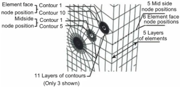
In principle, for each element layer along the thickness, the analysis will give out 10 val-ues for five element contours on element faces and 5 valval-ues for mid side node positions. These include the 5 rings of nodes of the quadratic element edges plus the 5 mid-side node rings. However, the output in the *.dat file is always for five contours averaged be-tween mid-side nodes and edge nodes. The mid-side nodes are always present in 20 node quadratic brick elements. The 3D model consists of five layers of elements in that make up the thickness of the specimen (each layer being 0.5 mm). The outer most layers gives lower values due to plane stress condition. There are 11 parallel sets of node rings making up the thickness of the specimen. Six rings on the element faces and five on the mid-sides. Thus we have a total of 55 J-integral values for each analysis carried out. In the present paper only the values of the last ring of nodes are considered (after convergence). The 11 values (11 layers of contour rings) are then averaged to find out the desired J-integral. The value of J-integral at the first contour, closest to the singularity, is never considered because they may give erroneous results due to large strains[6,9]. The contours are explained in detail in
Fig. 10.
All in all 50 analyses are carried out for the rectangular specimen comparison pur-poses, 5 analyses for the dog bone specimens and 25 analyses for the sensitivity analysis. 3.2 Rectangular specimens
The rectangular specimens, as described previously have been analyzed for verifi-cation and comparison of the method of FEA used in this analysis and by other researchers[3°5].
Fig. 10 Positions of the contours in the speci-men numerical model
The stress intensity factor in a body (Fig. 1) loaded by a force F leading to a nominal stress æ = F/BW , is given by
KI= æpºaf (a/W ) (4)
where f(a/W ) is the geometric correction factor. During the numerical simulation the software gives an output of the KI values. From these values the f(a/W ) can be deduced
from Eq. (2). Table 2 presents all the values of the correction factors. The graph in Fig. 11 represents the variation of the geometric correction factor as a function of the ratio of the crack length to the specimen width.
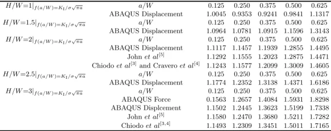
Table 2 Values of the correction factor f (a/W ), comparison with literature
H/W =1|f (a/W )=KI/æpºa a/W 0.125 0.250 0.375 0.500 0.625
ABAQUS Displacement 1.0045 0.9353 0.9241 0.9841 1.1317 H/W =1.5|f (a/W )=KI/æpºa a/W 0.125 0.250 0.375 0.500 0.625
ABAQUS Displacement 1.0964 1.0781 1.0915 1.1596 1.3143 H/W =2|f (a/W )=KI/æpºa a/W 0.125 0.250 0.375 0.500 0.625
ABAQUS Displacement 1.1117 1.1457 1.1939 1.2855 1.4495 John et al[5] 1.1292 1.1555 1.2023 1.2875 1.4471
Chiodo et al[3]and Cravero et al[4] 1.1243 1.1577 1.2099 1.3009 1.4605
H/W =2.5|f (a/W )=KI/æpºa a/W 0.125 0.250 0.375 0.500 0.625
ABAQUS Displacement 1.1774 1.2352 1.3138 1.4371 1.6186 H/W =3|f (a/W )=KI/æpºa a/W 0.125 0.250 0.375 0.500 0.625
ABAQUS Force 0.1563 1.2657 1.4084 1.5931 1.8298 ABAQUS Displcement 1.1502 1.2445 1.3623 1.5199 1.7338 John et al[5] 1.1580 1.2470 1.3680 1.5211 1.7282
Chiodo et al[3,4] 1.1493 1.2309 1.3451 1.5011 1.7165
The lower set of curves represents the correction factors for H/W =2 and the up-per set represents the curves for H/W =3. The correction factors obtained under diÆer-ent conditions of applied uniform force and applied uniform displacement have been rep-resented by the names ABAQUS Force and ABAQUS Displacement on the graph respec-tively. These curves have been subsequently compared with the calculations done by John et al[5], Chiodo et al[3] and Cravero et al[4]
using procedures described previously. The two authors have used an applied uniform displacement boundary condition.
The comparison of the graphs clearly shows that the applied displacement
bound-Fig. 11 Verification of the numerical analy-sis method on standard rectangular SE(T)C specimens & comparison with
publications
ary condition correlates very well in comparison to these authors, with the error ranging from 0.25% for a/W =0.125 to 1.5% for a/W =0.625. Whereas the error in readings at the same positions goes up to 8% for applied force boundary conditions.
Being an asymmetric specimen with respect to the force axis, the applied force boundary condition tends to add a bending moment at the crack tip. This has been analyzed in detail by Cravero et al [4] for pin loaded SE(T) specimens. In fixed grip specimens, the reaction
of this moment is present on the grips which, being very rigid as compared to the specimen, do not deform considerably. This has an eÆect of closing the crack thus reducing the values of the correction factors.
In view of the above discussion and the experimental conditions analyzed in section 2.2.3, it was decided to analyze the dog bone specimen with the applied displacement boundary condition only.
Other H/W ratios have also been studied in order to understand the trend of evolution of SIF in short length specimens. Also, these dimensions may be pertinent in other non
standard testing conditions. They are presented in Table 2 as well. 3.3 Dog bone specimen
The correction factors for the dog bone specimen are calculated in the same manner as above for crack lengths corresponding to 0.125∑a/W ∑0.625. The values obtained for this specimen are given in the Table 3.
Table 3 Correction factor f(a/W ) for dog bone specimens a/W 0.125 0.250 0.375 0.500 0.625 f (a/W ) 1.1428 1.2363 1.3568 1.5088 1.7119
The expression calculated and the subsequently used in all the experiments is repre-sented by the fourth order polynomial:
f≥ a W ¥ = C1+ C2 ≥ a W ¥ + C3 ≥ a W ¥2 + C4 ≥ a W ¥3 + C5 ≥ a W ¥4 (5) where C1=1.0869, C2=0.2383, C3=1.983, C4=2.8373, C5=2.5771.
In Fig. 12, the values of f(a/W ) have been compared for the dog bone specimen and the standard rectangular SE(T)C specimen with H/W =3. It can be seen that the
f (a/W ) values for the dog bone specimen approach those for the rectangular specimen with H/W =3.
3.4 Sensitivity study of grip position
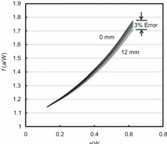
The justification of sensitivity study has been presented above. The sensitivity of grip installation position has been studied for crack lengths corresponding to 0.125∑a/W ∑0.625. The analysis has been carried out from 0 to 12 mm grip position, measured as shown in Fig. 9. The results of the sensitivity analysis are shown in Fig. 13. A maximum varia-tion of 3% can be observed at the extreme posivaria-tions. It should however be noted that this value in itself is very low, coupled with the fact that the sensitivity analysis has been
Fig. 12 Comparison of correction factors of dog bone specimen with standard rectangu-lar SE(T)Cof H/W = 3
Fig. 13 Sensitivity analysis of variation of spec-imen position in the grips
carried out for extreme position of the grips, whereas in reality only the half range of these conditions is encountered. To get an idea of acceptable limits of error, one needs to look at the comparison of diÆerent methods of calculation, analytical and numerical by Courtin et al [6] for standard C(T) specimens, showing up to 8% variation for the calculated values
by diÆerent authors. Thus an error of 3% is considered to be tolerable.
Thus the configuration of the test specimen and the experiment was not considered to be highly dependent on the variation of H/W due to the specimen grip position in a dog bone specimen. This seems to be in contradiction to the H/W sensitivity seen in rectangular specimens. The diÆerence in interpretation can be explained by the extra rigidity provided by the large ends of the dog bone specimen, Fig. 3.
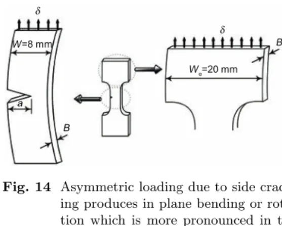
The H/W sensitivity in rectangular specimens is in fact the eÆect of in plane rotation in an SE(T)C specimen[4]. The longer specimens, being less rigid, will show a higher KI
value. It follows from in plane rotation of the specimen and the beam theory that the resistance to the moment, produced by the non symmetric loading, would be proportional to the moment of inertia or BW3, where W is the width of the specimen and B is its
thickness as shown in Fig. 14.
Applying the above explanation to our specimen with W =8 mm inside the gauge length and We=20 mm at the ends (Webeing
the width of the ends) the ratio of resistance to bending by the non symmetric loading in the gauge length to the specimen grip ends would be as follows:
¡ =≥We/W
¥3
ª
= 16 (6)
This shows that the specimen ends that are gripped by the machine are almost 16 times as rigid as the gauge length as regards to the in plane bending, hence the apparent non sensitivity of the position of the grips on the values of KI of the specimens.
Fig. 14 Asymmetric loading due to side crack-ing produces in plane bendcrack-ing or rota-tion which is more pronounced in the gauge length as compared to the spec-imen ends
In light of the above discussion it can be safely said that the minor changes in the installation position of the specimens will not show a marked error on the results of the experiments that were performed on these specimens. Also it was observed with experience that the dispersion of the data from the experiments is su±ciently high to render these diÆerences un-noticeable.
4 Experimental Validation
The SIF on SE(T)C specimens was used to determine the FCGR for a hot work tool
steel, AISI H11. The steel is a double tempered martensitic tool steel quenched and double tempered to 47HRC. The details of the experiments and material are given in the reference[1]. Here a comparison is presented with the FCGR curve of the same material,
with similar material properties, determined using C(T)25B12 specimens[11] as shown in
diÆerent initial stock sizes.
It can be seen from Fig. 15, that the two methods of determining the FCGR give re-markably similar results and trends, with the exact same slope of the Paris curve. The slight diÆerence may be due to the diÆerence of thickness of the specimens (2.5 mm for the SE(T)C and 25 mm for the C(T)
spec-imens). Also this may be due to the dif-ferences in microstructure due to diÆerent initial stock sizes from where the specimens were prepared.
This comparison in Fig. 15 proves be-yond any doubt that the method of sim-ulation of the SIF (for SE(T)C) by
nu-merical simulations the is valid and gives
Fig. 15 Comparison of Paris curves of two specimen geometries, SE(T)C and
C(T)25B12 specimens
good correlation to the analytical formulae used in determining the SIF for C(T) specimens, especially when used for FCGR purposes. However, one has to be careful to take the necessary precautions in applying the right boundary conditions in the numerical simulation methods.
5 Conclusions
In this paper, the experimental constraints impose a need to use a non standard SE(T)C
specimen configuration. The calculation process follows the energetic calculation of the domain integral J at the crack tip and its interpretation into the KI values in the elastic
domain. The analyses have been presented as three groups used in order to verify (1) the validity of the method, (2) the actual analysis of the specimen, and (3) the eÆect of experimental errors on the interpretation of the experimental data.
The results revealed that the domain integral method of KI calculation by using the
software ABAQUS/StandardTM are reliable when compared to work done by other
re-searchers using diÆerent software packages and diÆerent calculation methods. Two H/W configurations of 2 and 3 were analyzed in this paper. The comparison has been carried out for two types of end conditions with applied uniform force or applied uniform displacement. The applied displacement end condition was found to be satisfactory and closer to the real experimental conditions. The expression of KIfor the dog bone specimen was determined
using this condition.
EÆects of variation in specimen position while installing are studied. A sensitivity analysis of the variation was carried out. Due to the rigidity of the specimen ends there is not much eÆect of this variation (only 3% at extreme positions) and that the expression of KI calculated for specimens remains valid in real experimental conditions.
The numerically calculated and verified SIF is then applied on the FCGR of an AISI H11 tool steel. The results show an excellent correlation of results obtained for 2.5 mm thick SE(T)Cspecimens when compared with the FCGR for 25 mm thick C(T) specimens.
Numerically calculated SIF is used for the 2.5 mm SE(T)C specimen, while standard
REFERENCES
[1] M. Shah, C. Mabru, C. Boher, S. Leroux and F. Rezai-Aria, Adv Eng Mater 11 (2009) 746
[2] M. Shah, C. Mabru, C. Boher, S. Leroux and F. Rezai-Aria, Tool Steels (Aachen, Germany, 2009) p.83 [3] M.S. Chiodo, S. Cravero and C. Ruggieri. Stress Intensity Factors for SE (T) Specimens, Technical
Report BT-PNV-68 (Faculty of Engineering, University of Sao Paulo, 2006) [4] S. Cravero and C. Ruggieri, Eng Fract Mech 74 (2007) 2735
[5] R. John and B. Rigling, Eng Fract Mech 60 (1998) 147
[6] S. Courtin, C. Gardin, G. Bezine and H.B.H. Hamouda, Eng Fract Mech 72 (2005) 2174 [7] D.R.J. Owen and A.J. Fawkes, Eng Fract Mech (1983) 305
[8] J.R. Rice, J Appl Mech 35 (1968) 379
[9] K. Hibbit and I. Sorensen, ABAQUS Users’ Manual, Version 6.5 (2002) [10] R. Barsoum, Int J Numer Meth Eng 10 (1976) 25