A 2D vertical finite volume solver using a level set approach for simulating free surface incompressible flows

Texte intégral

(1)Vol 2009-3. ISSN 0035-3612. CONTENTS A 2D vertical finite volume solver using a level set approach for simulating free surface incompressible flows S. Detrembleur, B.J. Dewals, S. Erpicum, P. Archambeau, M. Pirotton. Performance and emission characteristics of a Diesel engine operating on cottonseed oil methyl ester Y.V. Hanumantha Rao, Ram Sudheer Voleti, A.V. Sitamara Raju, P. Nageswara Reddy. Part load emission reduction in a direct injection Diesel engine through porous medium combustion technique C. Kannan, P. Tamilporai. Experimental investigation of turbulent heat transfer in a horizontal tube with longitudinal strips S.N. Sarada, K.K. Radha, A.V.S. Raju. Information.

(2) Vibrations & Acoustics What we do … For your workers : noise and vibrations exposure quantification and contribution analysis. For your environment : noise and vibrations measurements. For your products and processes : Vibro-acoustics studies on machines (design and maintenance). For you : Training and consciousness-raising MoDyVA offers consulting services in acoustics and vibrations. Our goal is to help companies having noise and vibrations problems at the workplace and in the environment. We also assist our customers to design less vibrating and more silent products. You’re looking for solutions in vibrations and acoustics ? Please contact us or visit our website : With the support of the Walloon Region. +32 (0)65 37 41 80 +32 (0)476 672 111 philippe.brux@MoDyVA.be www.MoDyVA.be. c/o Faculté Polytechnique de Mons. Rue de Houdain, 9 B-7000 Mons BE 882.779.875.

(3) ISSN 0035-3612. Vol 2009-3. EUROPEAN JOURNAL OF. ECHANICAL AND ENVIRONMENTAL ENGINEERING BSMEE - Belgian Society of Mechanical and Environmental Engineering 2 Rue Hobbemastraat B 1000 Brussels, Tel 32-2-7376553, Fax 32-2-7376547 E-mail : Kristof.harri@rma.ac.be, www.bsmee.be, www.eneest.eu. Aims and Scope of the Journal The European journal of Mechanical and Environmental Engineering welcomes papers on all aspects of mechanical engineering. Topics include, but are not limited to, machine elements, machine construction, manufacturing technology, tribology, vibrations, environmental testing engineering, mechanical. power engineering, mechanical and thermal energy conversion, heat and fluid flow engineering. The journal also accepts papers of interdisciplinary nature, for example mechatronics, robotics, electronic and optical methods in mechanical and production engineering. The journal especially welcomes papers on environ-. mental engineering, i.e. on the influences of environmental factors on systems or on the interaction of systems with their environment, including security and safety aspects. Essential for acceptance is howeverthat mechanical engineering forms the core of a submitted paper.. Editorial Board Chairman Prof. Y.Baudoin, Royal Military Academy (BE) Editor Dr Ir K.Harri, BSMEE Secretary Members Prof JC Samin, Université Catholique de Louvain-La-Neuve. Prof P.Kool, Vrije Universiteit Brussel Prof S. Vanlanduit, Vrije Universiteit Brussel Prof B. Lauwers, Katholieke Universiteit Leuven Prof O. Verlinden, Faculté Polytechnique de Mons Prof P.Dehombreux, Faculté Polytechnique de Mons Prof B.Donnay, ISIL, Liège. Scientific Committee Prof C.Bostater, Florida Institute of Technology Prof B.Kiss, Budapest University of Technology Prof I.Dorofteï, Technical University of Iasi A. Charki,LASQUO-ISTIA, France Prof G.Muscatto , University of Catania Prof R.Molfino, Genova University Prof M.Armada, CSIC-IAI, Madrid Prof P.Kopacek, HUT Vienna Prof M.Maly, ME Institute of Technical University,Liberec Dr Karl-Friedrich Ziegahn, Forschungszentrum Karlsruhe. Prof B.-R. Höhn, TU München Prof K.Berns, University of Kaizerslautern Prof P.Regtien, University, Twente Prof A. Maslowski, Technical University Warschau Prof V.Gradetski, Institute for Problems in Mechanics, Moscou Prof. Håkan Torstensson, CEEES, Sweden Prof JC Golinval, Université de Liège Prof E.Dick, Universiteit Gent Prof R.Van den Braembussche,Von Karman Institute Prof A.Winffield, University of Bristol. 3.

(4) European Journal of Mechanical and Environmental Engineering. Volume 2009-3. A 2D vertical finite volume solver using a level set approach for simulating free surface incompressible flows a. S. Detrembleura, B.J. Dewalsa,b, S. Erpicuma, P. Archambeaua, M. Pirottona Unit of Hydrology, Applied Hydrodynamics and Hydraulic Constructions (HACH), ArGEnCo, University of Liege, Chemin des Chevreuils 1 B52/3+1, 4000 Liege, Belgium Email: sylvain.detrembleur@ulg.ac.be b Postdoctoral Researcher of the Belgian Fund for Scientific Research (F.R.S-FNRS). Abstract In order to solve the Navier-Stokes equations in the case of free surface incompressible flows, a method has been developed on the basis of the finite volume technique applied to a 2D Cartesian grid in the vertical plane. The projection method has been adopted to solve the water phase. The air phase is not solved explicitly but a weighted linear extrapolation of the velocity field computed in water is used, ensuring a divergence free velocity field in the air. The interface tracking is ensured by a level set approach. The numerical implementation of the projection method is carried out based on an original splitting of the unknowns for the transport step, achieving first or second order space accuracy. The projection step is carried out by solving the Poisson’s equation thanks to the iterative GMRES solver. Time integration is ensured by Runge-Kutta schemes. Moreover, the viscous diffusive terms are integrated into the model allowing the explicit computation of internal losses. The implemented model was first validated for pressurized flows based on benchmarks coming from literature. Next, the solver has been validated for both steady and unsteady free surface flows. An industrial application used to reduce damp wind-induced vibrations of high chimneys is illustrated by an experimental sloshing tank.. Keywords: Navier-Stokes equations, finite volume, free surface flow, projection method, level set.. 1. Introduction When modeling hydraulic structures, engineers need to conduct studies both at large scale and at smaller scales. Numerical studies at large scales can hardly be carried out using 3D models because of the high computational time needed. On the other hand, standard depth-averaged approaches enable to achieve accurately this goal but they remain valid only at a certain distance from the hydraulic structure and not in their near-field. In the vicinity of the structure, the assumptions on which depth-averaged models rely, such as the hydrostatic pressure distribution, are no more verified. In particular, vertical velocities may not be neglected anymore compared to the horizontal ones.. In such cases, explicitly discretized models on the water depth are needed to obtain accurate hydrodynamic results in the vicinity of the structure. While 3D models may be exploited, 2D vertical models also succeed to provide valuable information and require less computation time. For many applications, it is consequently relevant to opt for a reliable 2D vertical model, enabling to accurately describe the local flow patterns. Many real-world structures contain geometric singularities such as outfalls or local topographic steps. In addition, such singularities are often connected to a free surface flow, which constitutes an additional numerical challenge. The mathematical and computational model presented in this paper handles incompressible flows with free surface. The model has been successfully tested on a number of benchmarks.. 4.

(5) European Journal of Mechanical and Environmental Engineering The developed computer program is embedded in the modeling system WOLF, entirely developed at the University of Liege by the research unit HACH. This modeling system includes several components, solving hydrological run-off [1], flows in rivers and sewage networks [2], two-dimensional shallowwater flows [3,4,5,6,7,8], as well as 2D vertical incompressible free surface flows (WOLF2DV) as detailed in this paper. All developed computer codes are based on a similar algorithmic architecture. The finite volume method applied to structured grids is systematically used. Constant or linear reconstruction of unknowns guarantees first or second order space accuracy. Moreover, time integration is ensured by standard Runge-Kutta schemes up to four steps. Section 1 describes the basic principles governing the dynamics of flows in the vertical plane, including the Navier-Stokes equations and the equation used for free surface tracking. A brief review of the numerical approach used to solve these equations is provided. The projection method initially developed by Chorin [9] is also depicted. Section 2 details the space and time discretizations used for the transport step, as well as the implicit resolution of the Poisson's equation related to the projection step. Section 3 presents several benchmarks based on numerical and experimental results from the literature and showing the validity and accuracy of the implemented code for both pressurized and free surface flows.. 2. Governing equations The governing equations for the flow include the mass and momentum balances, while the free surface tracking is ensured by the Level Set approach [10]. The main assumptions underlying the model developed here are: - density is supposed to remain constant in time and space and is noted ρ0; - water is regarded as a Newtonian fluid, described by the tensor of shear viscous stresses; - the expression of the viscous stresses is simplified in accordance with Stokes hypothesis; - no surface tension is considered at the free surface. The following general form of the equations is obtained:. Volume 2009-3. ⎧→ → ⎪∇ ⋅ v = 0 ⎪ → → → ur 1 → ⎪∂ v ⎛ → → ⎞ → + v ⋅ ∇ v = − ∇ p + ∇ ⋅ ( ν ∇ v ) + f (1) ⎨ ⎜ ⎟ ρ0 ⎠ ⎪ ∂t ⎝ ⎪ ∂φ → → ⎪ + v ⋅ ∇ φ = 0 (Level set equation) ⎩ ∂t r where t is the time, v the velocity field, p the ur pressure, f the field of external volume forces, ν = μ / ρ0 the kinematic viscosity of the fluid, μ the dynamic viscosity or the shear stress viscosity of the fluid and φ the geometric distance to the free surface.. 2.1 Conservative form of the equations Using the hypothesis of incompressible fluid, one can rewrite equations (1) in a conservative form for the convective terms of the momentum equations. In order to rewrite similarly the level set equation in a conservative way, one must ensure that the continuity equation is also verified in the air domain. While it is definitely the case in the liquid phase, the same doesn’t automatically hold in the air. Therefore, in order to obtain a discrete divergence free velocity field in the air, a two-step procedure is followed. First, a linear extrapolation of the velocities computed in the water is exploited. Next, in order to restore the continuity, a correction step based on a Poisson’s equation is conducted. As a result, a global and local divergence free velocity field is computed everywhere with a second order accuracy in space. Finally, integrating the only considered external force (i.e. the gravity) into the pressure gradient, one can rewrite the set of equations (1) in the following form:. ⎧ ∂u ∂v ⎪ ∂x + ∂y = 0 ⎪ ⎪ ∂u ∂u 2 ∂uv 1 ∂p* ∂ 2u ∂ 2u + + + − ν ( + )=0 ⎪ ∂y ρ0 ∂x ∂x 2 ∂y 2 ⎪ ∂t ∂x (2) ⎨ 2 * 2 2 v v uv p v v ∂ ∂ ∂ 1 ∂ ∂ ∂ ⎪ + + + −ν ( 2 + 2 ) = 0 ⎪ ∂t ∂y ∂x ρ0 ∂y ∂x ∂y ⎪ ⎪ ∂φ + ∂uφ + ∂vφ = 0 ⎪ ∂t ∂x ∂y ⎩ where u and v are respectively the horizontal and vertical velocities while p* designates a conventional pressure that includes the hydrostatic pressure derived from gravity.. 5.

(6) European Journal of Mechanical and Environmental Engineering. 3. Projection method Following the projection method based on the Hodge theory [11], the resolution of the equations for incompressible flows is separated into two successive steps: the transport phase and the projection phase. In the transport phase, the projection of the Navier-Stokes equations in the vector space with null divergence is considered. As a result of the projection, the pressure gradients cancel out in the remaining form of the momentum conservation equations, which are solved to provide an approximate velocity field, noted ( u*, v *) :. ⎧ ⎡ ∂unun ∂unvn ⎛ ∂2un ∂2un ⎞⎤ n + −ν ⎜ 2 + 2 ⎟⎥ ⎪u* = u −Δt ⎢ ∂y ∂y ⎠⎦ ⎝ ∂x ⎪ ⎣ ∂x (3) ⎨ ⎡ ∂vnvn ∂unvn ⎛ ∂2vn ∂2vn ⎞⎤ ⎪ n ⎪v* = v −Δt ⎢ ∂y + ∂x −ν ⎜ ∂x2 + ∂y2 ⎟⎥ ⎝ ⎠⎦ ⎣ ⎩ where the superscript n refers to the previous time step. This approximated field does not yet verify the continuity equation. To restore the continuity at the next time step (noted n + 1), the approximate velocity field must be corrected based on the principle stated by the Hodge’s theorem. This correction depends on the gradient of a field q to be determined:. ⎧ * 1 ∂q*n +1 − Δ = u n +1 u t ⎪ ∂ ρ x ⎪ 0 ⎨ * n +1 ⎪v* − Δt 1 ∂q = v n +1 ⎪⎩ ρ0 ∂y. (4). An identification between (2) (written with an explicit Euler discretisation in time) and (4) shows that the unknown field q is simply the pressure of the fluid. Prior to deducing from (4) the velocity corrections needed to restore the continuity, it is necessary to compute the pressure. For this purpose, the divergence operator is applied to both members of equations (4) and both equations are summed. As a result, a relation is obtained between the Laplacian of the pressure and the divergence of the approximate velocity field, since the divergence of the velocity field at next time must be zero. This equation is more commonly known as the Poisson's equation and can be written as:. ∂ 2 p* ∂ 2 p* ρ0 ⎛ ∂u * ∂v* ⎞ + = + ⎜ ⎟ ∂x 2 ∂y 2 Δt ⎝ ∂x ∂y ⎠. (5). The resolution of this last one using the iterative GMRes method for linear systems provides the pressure field. The gradient of this pressure field. Volume 2009-3. enables then to modify the approximate velocity r field v * into a null divergence field following equation (4) where q equals p. This is known as the projection step. At the end of these operations, the new values of the variables are known and can be used as a predictor step in a Runge-Kutta scheme or directly as the result at the next time step for an Euler time integration.. 4. Free surface evolution After the Navier-Stokes equations being solved for the liquid phase, the location of the free surface needs to be updated using the level set technique. For this purpose, a divergence free velocity field needs to be computed in the fictitious air domain. Within a thin layer of air cells close to the interface, the velocities are extrapolated from those previously computed in the liquid phase. As presented by Sussman [12], the extrapolation is conducted following a four-step procedure: - for each considered cell in the air, tag the cells in the water that belong to a 5 × 5 stencil centered on the closest cell of the interface; - estimate by a least square approach the coefficients of a plane approximating the velocity field computed in the water; - compute the velocities in the air cell from the fitted plane approximation; - the extrapolated velocity field must be corrected to restore continuity in the air, by solving a Poisson’s equation with as a source term the divergence of the extrapolated velocity field. In addition, boundary conditions for the velocities are prescribed at the interface. The air cells located further from the interface should also verify the continuity equation but they don’t need to be extrapolated from the water domain. They progressively spoil the characteristic properties of the level set function, but without affecting the interface tracking. If needed, the level set function is redistanced at regular intervals.. 5. Boundary conditions Boundary conditions generally prescribed to solve the Navier-Stokes equations are velocities and pressure. In the present approach, the first ones are prescribed in the transport phase, while pressure boundary conditions are prescribed at the stage of solving the Poisson’s equation. Pressure conditions are required both at outflow. 6.

(7) European Journal of Mechanical and Environmental Engineering boundaries and at the time-varying free surface. At the free surface boundary, they are prescribed with a second order accuracy and accounting for the real distance between the boundary and the location of the free surface given by the level set function. Boundary conditions are also applied to the level set function at inlets, based on a geometric linear extrapolation of values existing in the domain.. 6. Applications. Volume 2009-3. to 10,000 cells on the finest grid. A linear reconstruction of the unknowns is used to achieve a second order accuracy in space. For the finest grid, the horizontal velocity in a cross section at x = L / 2 and the vertical velocity at y = L / 2 were compared with the results of Ghia [13] for Re = 400 (Figure 2 and Figure 3) and for Re = 1000 (Figure 4 and Figure 5). The results show a very good adequacy between the reference data and the results of the present model. 1. 6.1. Driven cavity flow. 0.8. 0.4. 0.2 Ghia et Al. (1982) Wolf2DV Δx=1cm. 0 ‐0.4. ‐0.2. 0. 0.2 0.4 u/ULid. 0.6. 0.8. 1. Figure 2: Horizontal velocities for Re = 400 at x = L / 2. 0.4. Ghia et Al. (1982) Wolf2DV Δx=1cm. 0.2. 0. v/ULid. u = U Lid = 1m / s. 0.6. y/L. In order to validate the implemented projection method, the model was first tested for the simulation of a particular pressurized flow, namely a driven cavity flow. The considered geometry is a square box of length L (Figure 1). The lid of the box moves at a constant velocity U Lid , while a no-slip boundary condition is prescribed on the three other sides. In addition, all normal velocities on the boundaries are set to zero. The initial conditions correspond to a fluid at rest everywhere in the box. Two different values for the kinematic viscosity were considered in order to simulate Reynolds numbers of 400 and 1000. Since the characteristic length and lid velocity equal unity, the Reynolds Number is simply expressed by Re = ν –1 and the corresponding kinematic viscosity values are 2.5 × 10-3 and 10-3 m²/s. v=0. ‐0.2. ‐0.4. L. u=0 v=0. ν = 2,5.10 / ν = 1.10 −3. u=0 v=0. −3. ‐0.6. u=0 v=0. 0. 0.2. 0.4. x/L. 0.6. 0.8. 1. Figure 3: Vertical velocities for Re = 400 at y = L / 2. y x. L. Figure 1 : Geometry, boundary and initial conditions for the driven cavity flow. Simulation results show a flow pattern characterized by the development of a vortex in the box until reaching a steady state. The cell sizes used are either 1 cm, 2 cm or 4 cm, leading. 7.

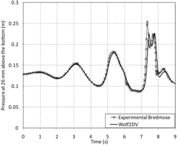
(8) European Journal of Mechanical and Environmental Engineering. Volume 2009-3. 1. 6.2. Sloshing in an open tank 0.8. y/L. 0.6. 0.4. 0.2 Ghia et Al. (1982) Wolf2DV Δx=1 cm ‐0.4. ‐0.2. 0. 0.2 0.4 u/ULid. 0.6. 0.8. 1. Figure 4: Horizontal velocities for Re = 1000 at x = L / 2. 0.6. Ghia et Al. (1982) Wolf2DV Δx=1 cm. 0.4. v/ULid. 0.2 0. ‐0.2 ‐0.4 ‐0.6 0. 0.2. 0.4. x/L. 0.6. 0.8. 1. Figure 5: Vertical velocities for Re = 1000 at y = L / 2. The L1 error versus the cell size is plotted in Figure 6, confirming the second order accuracy of the method. The L1 error is defined as:. L1 =. 1 N. ∑. N. δ i ,exact − δ i ,computed. (6). δ i ,exact. i =1. 0.4. where δi,exact is the reference value, δi,computed the computational result and N the number of cells. Δx 0.01. 0.001 v. 0.1 1. u. 0.1. L1 error. Slope of 1/Δx². Horizontal tank acceleartion (m/s²). 0. The second validation example refers to the experiments of Bredmose et al. [14], consisting of a rectangular glass tank of size 1.48 × 0.4 × 0.75 m (length × width × height) fastened on a support table and shaken in the horizontal direction. This kind of tank is often used in order to damp wind-induced vibrations of high chimneys. The tank must be designed in such a way that the movement of the water contained in the tank slows down the movement of the chimney. The example described hereafter shows the ability of the present model to simulate such free surface transient flows and shows the applicability of the model for the design of such hydraulic dampers. Initially, the tank is motionless and filled with water with a depth of 155 mm. The support table is moved horizontally (along the longest side of the container) according to the driving signal shown in Figure 7. In the experiments, the profiles of the water surface were recorded using a stationary video camera, and the pressure of the water on the left wall of the tank was measured with a pressure transducer. In our model, the frame of reference is associated with the tank. Surface tension effects are neglected. Simulations were performed on a 5 mm grid with a free-slip boundary condition on the tank walls. The acceleration of he tank is modeled by an external force that act in the momentum equation along the x axis. Figure 8 shows the pressure evolution on the left wall of the tank, 26 mm above the floor. There is a slight different phase shift between the experimental and numerical curves but the overall agreement is satisfactory.. 0. ‐0.4. ‐0.8. ‐1.2 0. 0.01. Figure 6: Error L1 for a grid size of 1 cm, 2cm and 4 cm (both logarithmic axis). 1. 2. 3. 4 5 Time (s). 6. 7. 8. 9. Figure 7: Horizontal tank acceleration as a function of time.. 8.

(9) European Journal of Mechanical and Environmental Engineering. Pressure at 26 mm above the bottom (m). 0.3. [5]. 0.25. 0.2. [6] 0.15. 0.1. 0.05. [7] Experimental Bredmose Wolf2DV. 0 0. 1. 2. 3. 4 5 Time (s). 6. 7. 8. 9. Figure 8: Pressure histories on the left vertical wall, 26 mm above the floor.. 7. Conclusion A second order accurate algorithm for solving free surface flows in a 2D vertical plane has been presented. It enables to solve the Navier-Stokes equation in water while a divergence free velocity field is constructed in the fictitious air domain. The interface tracking is achieved using the level set method. The code developed has been validated for a number of benchmarks involving both pressurized and free surface transient flows.. [8]. [9]. [10]. References [1]. [2]. [3]. [4]. Khuat Duy, B., P. Archambeau, S. Erpicum, B. J. Dewals et M. Pirotton. Modélisation hydrologique à grande échelle des zones imperméables égouttées. Houille Blanche-Rev. Int., 2009, Accepté. Kerger, F., P. Archambeau, S. Erpicum, B. J. Dewals et M. Pirotton. Simulation numérique des écoulements mixtes hautement transitoires dans les conduites d'évacuation des eaux. Houille BlancheRev. Int., 2009, Accepté. Roger, S., B. J. Dewals, S. Erpicum, M. Pirotton, D. Schwanenberg, H. Schüttrumpf et J. Köngeter. Experimental und numerical investigations of dikebreak induced flows. J. Hydraul. Res., 2009. in press. Erpicum, S., T. Meile, B. J. Dewals, M. Pirotton et A. J. Schleiss. 2D numerical flow modeling in a macro-rough channel. Int. J. Numer. Methods Fluids, 2009. published online: 13 Feb 2009.. [11]. [12]. [13]. [14]. Volume 2009-3. Erpicum, S., B. J. Dewals, P. Archambeau et M. Pirotton. Dam-break flow computation based on an efficient flux-vector splitting. J. Comput. Appl. Math., 2009. accepted. Dewals, B. J., S. A. Kantoush, S. Erpicum, M. Pirotton et A. J. Schleiss. Experimental and numerical analysis of flow instabilities in rectangular shallow basins. Environ. Fluid Mech., 2008, 8. 3154. Dewals, B. J., S. Erpicum, P. Archambeau, S. Detrembleur et M. Pirotton. Hétérogénéité des échelles spatio-temporelles d'écoulements hydrosédimentaires et modélisation numérique. Houille Blanche-Rev. Int., 2008, 5. 109-114. Dewals, B. J., S. Erpicum, P. Archambeau, S. Detrembleur et M. Pirotton. Depth-integrated flow modelling taking into account bottom curvature. J. Hydraul. Res., 2006, 44. 787-795. Chorin, A. J. Numerical method for solving incompressible viscous flow problem. Journal of Computational Physics, 1967, 2. 12-20. Sethian, J. A. Level Set Methods and Fast Marching Methods - Evolving Interfaces in Computational Geometry, Fluid Mechanics, Computer Vision and Materials Science. Berkeley, Cambridge University Press. 1999 Denaro, F. M. On the application of the Helmholtz-Hodge decomposition in projection methods for incompressible flows with general boundary conditions. Internatinal journal for numerical method in fluids, 2003, 43. 43-69. Sussman, M. A second order coupled level set and volume-of-fluid method for computing growth and collapse of vapor bubbles. Journal of Computational Physics, 2003, 187. 110-136. Ghia, U., K. N. Ghia et C. T. Shin. HighRe solutions for incompressible flow using the Navier-Stokes equations and a multigrid method. Journal of Computational Physics, 1982, 48(3). 387411. Bredmose, H., M. Brocchini, D. H. Peregrine et L. Thais. Experimental investigation and numerical modelling of steep forced water waves. Journal of Fluid Mechanic, 2003, 490. 217-249.. 9.

(10) European Journal of Mechanical and Environmental Engineering. Volume 2009-3. Performance and emission characteristics of a diesel engine operating on cottonseed oil methyl ester Y.V. Hanumantha Raoa, Ram Sudheer Voletia, A.V. Sitarama Rajub, P. Nageswara Reddyc Department of Mechanical Engineering, K.L. College of Engineering, Green Fields, Guntur Dt, Fax: +918645 247249, Andhra Pradesh-522502, India Email: mechanicalmighty@yahoo.co.in b Department of Mechanical Engineering, J.N.T.U College of Engineering, Kakinada, Andhra Pradesh-533003, India Email: avsr_raju2005@yahoo.com c Principal, BITS, Narasampet, Warangal Dt, Andhra Pradesh-506331, India Email: nageswara_preddy@rediffmail.com. a. Abstract The scarce and rapidly depleting conventional petroleum resources have promoted research for alternative fuels for internal combustion engines. In view of this, the vegetable oil is a promising alternative fuel for diesel engines as it has several advantages. The high viscosity causes some problems in atomization of injector systems and combustion in cylinders of diesel engines. In present research, to decrease viscosity of raw cottonseed oil, cottonseed methyl ester is obtained by transesterification process. The fuel properties of cottonseed methyl ester such as kinematic viscosity, calorific value, flash point, fire point, carbon residue and density were found. A single cylinder, four stroke, constant speed, water cooled, direct injection diesel engine was used for the experiments. The acquired data were analyzed for various parameters such as brake thermal efficiency, specific fuel consumption and exhaust gas temperature. Results indicated that B25 fuel has closer performance to mineral diesel. The brake thermal efficiency for biodiesel and its blends is found to be slightly higher than that of diesel fuel at tested load conditions. For cottonseed biodiesel and its blended fuels, the exhaust gas temperature increased with increase in load. The engine experimental results showed that exhaust emissions including CO, CO2 and HC emissions were reduced for all biodiesel mixtures. However, a slight increase in oxides of nitrogen (NOx) emission was experienced for biodiesel blends.. Keywords: cottonseed oil, biodiesel, transesterification, diesel engine, performance, emissions.. 1. Introduction The high energy demand in the industrialized world as well as in the domestic sector and pollution problems caused due to the widespread use of fossil fuels make it necessary to develop renewable energy sources. From the point of view of protecting global environment and concerns for long-term energy security, it becomes necessary to widen alternative fuels with properties comparable to petroleum based fuels. The rapid depletion of petroleum reserves and fluctuating oil prices has led to the search for alternative fuels. This was the basic motivation behind the research in this paper. Non edible oils are promising fuels for agricultural applications. Vegetable oils have properties comparable to diesel and can be used to run compression. ignition engines with little or no modifications. For diesel engines, a significant research effort has been directed towards using vegetable oils and their derivatives as fuels [1]. Most of the investigations reported in the literature on the usage of vegetable oil as engine fuels have emphasized modifying the oil fuels to work in existing engine designs. Studies have shown that the usage of vegetable oils in neat form is possible but not preferable [4-12]. The high viscosity of vegetable oils and the low volatility affects the atomization and spray pattern of fuel, leading to incomplete combustion and severe carbon deposits, injector choking and piston ring sticking. There are different methods used for improving fuel properties and decreasing viscosity and density of oils such as dilution of vegetable oils with solvents, pyrolysis,. 10.

(11) European Journal of Mechanical and Environmental Engineering microemulsification with alcohols and transesterification. Among the methods that had been investigated, transforming the oils to their corresponding esters proved to be the best alternative. The fuel characteristics of these esters were much closer to those of diesel fuel than the vegetable oils. To reduce the viscosity, transesterification is the commonly used commercial process to produce clean and environmental friendly fuel. However, this adds extra cost of processing because of the transesterification reaction involving chemical and process heat inputs [3]. The difference between biodiesel and the diesel fuel is concerned with oxygen content. Biodiesel contains 10–12% oxygen in weight basis and this lowers the energy content. The lower energy content causes reductions in engine torque and power. Biodiesel containing oxygen reduces exhaust emissions such as CO, HC and Smoke mainly due to the effect of complete combustion. In the present investigation, cottonseed oil (C.S.O), that is non-edible oil, was considered as a potential alternative fuel for compression ignition engines. Three blends were obtained by mixing diesel and cottonseed methyl ester in the following proportions by volume: 75% Diesel+25% Esterified C.S.O, 50% Diesel+50% Esterified C.S.O and 25% Diesel+ 75% Esterified C.S.O. For comparison purposes experiments were also carried out on 100% Esterified C.S.O and diesel fuel.. 2. Methods and measurements The conversion of Cottonseed oil into its methyl ester can be accomplished by the transesterification process. Transesterification involves, reacting the triglycerides of Cottonseed oil with methyl alcohol in the presence of a catalyst Sodium Hydroxide (NaOH) to produce glycerol and fatty acid ester.. Volume 2009-3. 2. Reaction. The alcohol/catalyst mix is then charged into a closed reaction vessel and 1000ml Cottonseed oil is added. Excess alcohol is normally used to ensure total conversion of the fat or oil to its esters. 3. Separation of glycerin and biodiesel. Once the reaction is completed, two major products exist: glycerin and biodiesel. The quantity of produced glycerin varies according the oil used, the process used, the amount of excess alcohol used. Both the glycerin and biodiesel products have a substantial amount of the excess alcohol that was used in the reaction. The reacted mixture is sometimes neutralized at this step if needed. 4. Alcohol Removal. 5. Glycerin Neutralization. The glycerin byproduct contains unused catalyst and soaps that are neutralized with an acid and sent to storage as crude glycerin. In some cases the salt formed during this phase is recovered for use as fertilizer. In most cases the salt is left in the glycerin. 6. Methyl Ester Wash. The most important aspects of biodiesel production to ensure trouble free operation in diesel engines are complete reaction, removal of glycerin, removal of catalyst, removal of alcohol and absence of free fatty acids.. 2.1 Measurement of properties The physical and chemical properties of Cottonseed oil are measured and tabulated in Table 1. Performance of CI engine greatly depends upon the properties of fuel among which viscosity, density, cetane number, calorific value, etc are very important. Calorific value and viscosity are measured by bomb calorimeter and redwood viscometer respectively. The flash point and fire point are determined by Pensky-Martens apparatus closed-cup method. The pour point is measured by cooling process. Carbon residue is measured by Conradson method. The cetane number is determined by measuring the Aniline point.. 3. Experimental setup The production of biodiesel by transesterification of the oil generally occurs using the following steps: 1. Mixing of alcohol and catalyst. For this process, a specified amount of 450ml methanol and 10gm Sodium Hydroxide (NaOH) were mixed in a round bottom flask.. The engine used for this experimental investigation was a single cylinder four stroke naturally aspirated water cooled diesel engine having 5 BHP as rated power at 1500 rpm. The engine was coupled to a brake drum dynamometer to measure the output. Fuel flow rates were timed with calibrated burette. Exhaust. 11.

(12) European Journal of Mechanical and Environmental Engineering gas analysis was performed using a multi gas exhaust analyzer. The pressure crank angle diagram was obtained with help of a piezo electric pressure transducer. A Bosch smoke pump attached to the exhaust pipe was used for measuring smoke levels. The specifications of the engine are shown in Table 1. The total experimental set up is shown in Figure 1.. Volume 2009-3. 3.1 Experimental procedure Experiments were initially carried out on the engine using diesel as the fuel in order to provide base line data. The cooling water temperature at the outlet was maintained at 70oC. The engine was stabilized before taking all measurements. Subsequently experiments were repeated with methyl ester of Cottonseed oil for comparison. In all cases the pressure and crank angle diagram was recorded and processed to get combustion parameters. The performance and emissions data were then analyzed for all experiments and the results are reported in the following section.. 4. Results and discussion. Figure 1: Schematic diagram of Experimental setup 1. Engine 2. Brake drum dynamometer 3. Biodiesel tank 4. Diesel tank 5. Burette 6. Three way valve 7. Air box 8. Manometer 9. Air flow direction 10. Exhaust gas analyzer 11. Smoke meter 12. Exhaust flow Manufacturer. Kirloskar engines Ltd, Pune, India Engine type Vertical, four stroke, single cylinder, constant speed, compression ignition Rated power 3.68 kW at 1500 rpm Bore & stroke 80 & 110 mm BHP of engine 5 Swept volume 562cc Compression ratio 16.5:1 Mode of injection Direct Injection Cooling system Water Table 1. Specifications of the engine. The physical and thermal properties of mineral diesel, cottonseed oil and cottonseed methyl ester are measured and tabulated in Table 2. Density, kinematic viscosity and carbon residue of cottonseed oil was found higher than diesel. The flash and fire points of cottonseed oil was quite high compared to diesel. It was observed that with the increase in percentage of biodiesel in various blends, flash point and fire point were increased. Hence, cottonseed oil is extremely safe to handle. Higher carbon residue from cottonseed oil may possibly lead to higher carbon deposits in combustion chamber of the engine [8]. Cottonseed oil has approximately 95% calorific value compared to diesel. Higher viscosity is a major problem in using cottonseed oil as fuel for diesel engines. However, this property was reduced with the help of transesterification process. Viscosity of cottonseed methyl ester is 4.0 cst at 40 oC. It is observed that viscosity of cottonseed oil decreases remarkably with increasing temperature and it becomes close to diesel at temperature above 90 oC. Cottonseed oil carries a higher cetane number than mineral diesel fuel. The cetane number measures a fuel’s combustion quality, and is determined by the ignition delay period. Higher number has been associated with reduced engine roughness and with lower starting temperatures for engines [11].. 12.

(13) European Journal of Mechanical and Environmental Engineering Sl. No. Property. Mineral diesel. 1. 2.. Density (kg/m3) Kinematic viscosity (mm2/sec), 40°C Flash point (°C) Fire point (°C) Pour point (°C) Calorific value (kJ/Kg) Carbon residue (% w/w) Cetane number Color. 840-842 2.44-2.71. 3. 4. 5. 6. 7. 8. 9.. Volume 2009-3. Cottonseed oil. Cottonseed methyl ester. ASTM method. 910-920 4.2-4.4. 880-890 3.8-4.0. D1298 D445. 71 228 195 D93 103 274 220 D93 -5 -6 -4 D97 45,343 42,150 41,680 D240 0.1 0.9-1.0 0.02 D189 48-56 52 48 D4737 Light yellow Light D1500-2 brown yellow Table 2. Fuel properties of mineral diesel, Cottonseed oil and Cottonseed methyl ester. 4.1 Brake power versus specific fuel consumption Specific fuel consumption (S.F.C) is calculated by fuel consumption divided by the rated power output of the engine. In Figure 2, it is observed that specific fuel consumption increases with percentage increase in blending of cottonseed methyl ester in diesel compared to mineral diesel. This trend was observed owing due to the fact that biodiesel blends have a lower heating value than mineral diesel [4]. The percent increase in specific fuel consumption was increased with decreased amount of diesel in the blended fuels. This may be due to higher density and lower calorific value of the biodiesel fuel as compared with diesel.. heating value of fuel. It is well known that brake specific fuel consumption is inversely proportional to the brake thermal efficiency. Brake thermal efficiency of biodiesel blends was found to be slightly higher than that of diesel fuel at tested load conditions. Figure 3 indicates that Esterified cottonseed oil gives less brake thermal efficiency compared to mineral diesel at tested load conditions. This is due to poor spray characteristics, poor air fuel mixing, higher viscosity and lower calorific value [11].. Figure 3: Variation of brake thermal efficiency with brake power. 4.3 Brake power versus exhaust gas temperature Figure 2: Variation of specific fuel consumption with brake power. 4.2 Brake power versus brake thermal efficiency Brake thermal efficiency is defined as actual brake work per cycle divided by the amount of fuel chemical energy as indicated by lower. The exhaust gas temperature gives an indication about the amount of waste heat going with exhaust gases. The exhaust gas temperature increased with increase in load and amount of blended biodiesel in the fuel. In Figure 4, it was observed that the exhaust gas temperature with mineral diesel and Esterified cottonseed oil is same. The exhaust gas temperature reflects on the status of combustion inside the combustion chamber. The reason for raise in the exhaust gas. 13.

(14) European Journal of Mechanical and Environmental Engineering temperature may be due to ignition delay and increased quantity of fuel injected. The exhaust gas temperature can be reduced by adjusting the injection timing/injection pressure in to the diesel engine [7].. Volume 2009-3. 4.5 Brake power versus CO2 The carbon dioxide (CO2) emission from the diesel engine with different blends is shown in Figure 6. The CO2 increased with increase in load conditions for diesel and decreased for biodiesel and its blended fuels. Esterified Cottonseed oil has lower CO2 emission compared to its blends and mineral diesel.. Figure 4: Variation of exhaust gas temperature with brake power. 4.4 Brake power versus CO Figure 6: Variation of CO2 with brake power If the combustion is incomplete due to shortage of air or due to low gas temperature, CO will be formed. The carbon monoxide (CO) emission from the diesel fuel with biodiesel blended fuels and biodiesel is shown in Figure 5. CO emission of all types of tested fuels was decreased with the increase in brake power. Carbon monoxide concentrations decreased by 18 and 24% when using B25 and B100, respectively, when compared to diesel fuel. The amount of CO emission was lower in case of biodiesel blended fuels than diesel because of the fact that biodiesel contained 11 per cent oxygen molecules [6]. This may lead to complete combustion and reduction of CO emission in biodiesel fuelled engine.. 4.6 Brake power versus NOX At higher power output conditions, due to higher peak and exhaust temperatures the NOx values are relatively higher compared to low power output conditions. Figure 7 also shows that NOx level was higher for biodiesel blends than mineral diesel fuel. This can be explained due to the presence of extra oxygen in the molecules of biodiesel blends. This additional oxygen was responsible for NOx emission. The reason for increase in NOx with respect to Esterified Cottonseed oil may be due to sustained and prolonged duration of combustion associated with reduction in combustion temperature [11]. Approximately 10% increase in NOx emission was realized with biodiesel blends. Reduction of NOx with biodiesel may be possible with the proper adjustment of injection timing and introducing to exhaust gas recirculation (EGR).. Figure 5: Variation of CO with brake power. 14.

(15) European Journal of Mechanical and Environmental Engineering. Volume 2009-3. 4. Conclusions. Figure 7: Variation of NOX with brake power. 4.7 Brake power versus Unburnt HC emissions The primary reason of the unburnt HC emission from CI engine is improper combustion and combustion of heavy lubricating oil. At higher power ouput conditions, the percentage of unburnt HC decreases with Esterified Cottonseed oil and its blended fuels compared to mineral diesel. Figure 8 shows that Esterified Cottonseed oil has low unburnt HC which leads to complete combustion of the fuel in the engine cylinder. It was found that particulate emission with B25 was lower than that of diesel fuel because neat biodiesel contains 10–12% extra oxygen, which resulted in better combustion and lower unburnt HC emission [10].. This work investigated the production of biodiesel from non edible cottonseed oil and performance study of single cylinder compression ignition engine with diesel fuel and biodiesel blends. The following conclusions are arrived based on the experimental results. Transesterification of cottonseed oil bring down the viscosity in close range to diesel. Biodiesel blends result in a slightly increased thermal efficiency as compared to that of diesel. The exhaust gas temperature is decreased with the methyl ester of cottonseed oil as compared to diesel. CO emission is low at higher loads for the cottonseed methyl ester and its blended fuels. Approximately 10% increase in NOx emission was realized with biodiesel blends. However, further studies can be carried out to decrease NOx emissions. Emission parameters such as CO, CO2 and HC were found to have increased with increasing proportion of cottonseed oil in the blends compared to diesel. As a result of all of the findings mentioned above, it can be concluded that cottonseed methyl ester can be partially (up to 20–25%) substituted for mineral diesel at most operating conditions in terms of performance parameters and emissions without any engine modification and preheating of the blends. On the whole it is concluded that the cottonseed methyl ester oil will be a good alternative fuel in diesel engines in rural areas for agriculture, irrigation and electricity generation.. Acknowledgements The authors are indebted to the financial support from Koneru Lakshmaiah College of Engineering, Vaddeswaram.. Figure 8: Variation of unburnt HC with brake power. 15.

(16) European Journal of Mechanical and Environmental Engineering. References [1] Altõn.R, An experimental investigation on use of vegetable oils as diesel engine fuels, Ph.D Thesis, Gazi University, Institute of Science and Technology, 1998. [2] Barnwal.S, Prospects of biodiesel production from vegetable oils in India, Renewable and Sustainable Energy Reviews, 9: 363–378, 2005. [3] Canakci.M, J.H, Van Gerpen, Biodiesel production from oils and fats with high free fatty acids, Trans. of ASAE, 44(6): 1429-1436, 2001. [4] Deepak Agarwal, Avinash Kumar Agarwal, Performance and emissions characteristics of Jatropha oil (Preheated and blends) in a direct injection compression ignition engine, Applied Thermal Engineering, 27: 2314–2323, 2007. [5] G.Amba Prasad Rao, P.Rama Mohan, Effect of supercharging on performance of a DI Diesel engine with cotton seed oil, Energy Conversion and Management, 44: 937–944, 2003. [6] Haldar SK, Ghosh BB, Nag A, Studies on the comparison of performance and emission characteristics of a diesel engine using three degummed non-edible vegetable oils, Biomass and Bioenergy, accepted, 2008. [7] Hanumantha Rao Y V, Ram Sudheer Voleti, Hariharan V S, Sitarama Raju A V, Jatropha oil methyl ester and its blends used as an alternative fuel in diesel engine, Int J Agric & Biol Eng, 1(2): 1-7, 2008. [8] Harrington, KJ, Chemical and physical properties of vegetable oil esters and their effect on diesel fuel performance, Biomass, 9(1): 1–17, 1987. [9] J.Narayana Reddy, Ramesh, Parametric studies for improving the performance of Jatropha oil-fuelled compression ignition engine, Renewable Energy, 31: 1994– 2016, 2006. [10] Md.Yousuf Ali, S.N.Mehd, P.R.Reddy, Performance and emission characteristics of a diesel engine with cottonseed oil plus diesel oil blends, International Journal of Engineering, 18(1), 2005. [11] M.N.Nabi, et al., Biodiesel from cotton seed oil and its effect on engine performance and exhaust emissions,. Volume 2009-3. Applied Thermal Engineering, accepted, 2008. [12] M.S. Kumar, Ramesh, An experimental comparison of methods to use methanol and Pongamia oil in a compression ignition engine, Biomass and Bio Energy, 25: 309-318, 2003. [13] S.P.Chincholkar, et al., Biodiesel as an Alternative Fuel for Pollution Control in Diesel Engine, Asian J. Exp. Sci., 19(2): 13-22, 2005. [14] Y Ali, M A Hanna, Alternative Diesel Fuels from Vegetable Oils, Bioresource Technology, 50: 153-163, 1994.. 16.

(17) European Journal of Mechanical and Environmental Engineering. Volume 2009-3. PART LOAD EMISSION REDUCTION IN A DIRECT INJECTION DIESEL ENGINE THROUGH POROUS MEDIUM COMBUSTION TECHNIQUE C.Kannana, P.Tamilporaib Department of Automobile Engineering, Sri Venkateswara College of Engineering, Post Bag No.3,Pennalur, Sriperumbudur – 602 105, Tamilnadu, India b Division of IC Engines,Department of Mechanical Engineering, CEG, Anna University, Guindy, Chennai – 600 025, Tamilnadu, India Email: kannancp@svce.ac.in a. Abstract The diesel engines are being extensively used in transport sector owing to their excellent fuel efficiency, low emissions of carbon dioxide (CO2), unburned hydrocarbons (UBHC) and carbon monoxide (CO). However, high emissions of nitrogen oxides (NOx) and particulate matter (PM) place the diesel engines on the down side. It is extremely complex to reduce both the emissions at the same time, because of the trade-off between NOx and PM emissions. Even though the implementation of high pressure injection and common rail system could reduce both NOx and PM emissions all together, the cost involved would be high and unaffordable for many engine producers and consumers. In this research work, a new combustion technique named as porous medium combustion has been proven to be proficient technique in reducing both NOx and PM emissions from the direct injection (DI) diesel engines.. Keywords: Porous medium, Combustion, Oxides of nitrogen, Particulate etc.. 1. Introduction Reduction in diesel engine emissions, in particular NOx and PM emission is becoming a serious problem to be tackled, as emission norms are getting more and more stringent. The effects of in-cylinder fuel-air mixture formation, combustion and chemical reaction process on exhaust emissions remain largely unexamined. On the other hand, it is well proven that a homogenous mixture results in a lower PM emission from diesel engines [1, 3]. Researchers are trying various technologies to accomplish homogenous mixture formation, combustion and subsequently lower PM emission. One such technique to realize homogenous mixture formation and lower PM emission from diesel engines is porous medium combustion [7]. Low NOx emission will be the supplementary benefit of porous medium combustion technique [5, 6].. types of engines, this practice is most often restricted to DI diesel engines. The most critical process in this technique is the fuel vapourization. Imperfections within this process directly influence the quality of the combustible fuel-air mixture, resulting in higher exhaust gas emissions of CO, NOx and UBHC [2]. Injecting the liquid fuels into the porous medium leads to an excellent evaporation and in turn, in the presence of oxygen, rapid and complete combustion as well. In this research work, the porous medium combustion was established in direct injection diesel engine with the inclusion of porous ceramic material into the space of the combustion chamber. The influence of the porous medium on the performance and emission characteristics of the engine under investigation was analyzed and compared with the conventional engine.. Even though, the porous medium combustion technique could be successfully implemented with wide variety of liquid fuels and different. 17.

(18) European Journal of Mechanical and Environmental Engineering. 2. Development medium engine. of. a. porous. Highly Porous ceramic material was selected for the purpose of developing the porous medium engine. High porosity made the medium to be transparent for gas flow, spray and flame. In general, the porous medium engine had been attained by the precise placement of porous ceramic material in either of the following locations: cylinder, engine head or piston. In this research work, the porous ceramic material was placed on the top of piston cavity and had been detained in its position through an appropriate locking mechanism. The photographic view of such a piston with porous medium implementation is shown in Figure 1. The chemical composition and mechanical properties of porous ceramic material are given in Table 1.. Volume 2009-3. injection (DI) diesel engine which was further coupled to an eddy current dynamometer. The main specifications of the test engine were given in Table 2. 5. 4 6. 15. 13. 7. 10. 3. 14. 8 1. 12 11. 9. 2. Figure 2: Experimental setup 1 - Diesel Engine 2 - Electrical dynamometer 3 - Dynamometer controls 4 - Air box 5 - U tube manometer 6 - Fuel tank 7 - Fuel measurement 8 - Pressure transducer 9 - TDC position sensor 10 - Charge amplifier 11-TDC amplifier circuit 12 - Analog to digital card 13 - Computer 14 - Exhaust gas analyzer 15 - AVL smoke meter Mark Model Type. Figure 1: Photographic view of the piston with porous medium implementation Cu Nominal 87.590.5. Fe C Sn 1.0 1.75 9.5 max max 10.5. Other 0.5. Density 6.4 -6.8 g/cc Porosity (% oil by vol.) 18 % K strength constant 26500 Tensile strength 96.5 MPa Elongation (% in once inch) 1% Yield strength in compression 75.8 MPa Table 1. The chemical composition and mechanical properties of porous ceramic material. 3. Experimental set up and test procedure The engine test up used for the experimental investigation is shown in Figure 2. The performance and emission tests were performed on a 4.4 kW, constant speed, single cylinder, four stroke, naturally aspirated, air cooled direct. Bore x Stroke (mm) Compression ratio Swept volume Rated Power Rated Speed Start of Injection Connecting rod length Injector operating pressure. Kirloskar TAF 1 Direct Injection, Air Cooled 87.5 x 110 mm 17.5 :1 0.661 L 4.4 kW 1500 rpm 23.40 before TDC 220 mm 250 bar. Table 2. Specifications of test engine In order to determine the engine torque, the shaft of the test engine was coupled to an electric dynamometer, which was loaded by an electric resistance. A strain load sensor was employed to determine the load on the dynamometer. The engine speed was measured by an electromagnetic speed sensor installed on the dynamometer. The fuel consumption rate of the engine was determined with a weighing scale having a sensitivity of 0.1 g and an electronic chronometer having a sensitivity of 0.1 s. The. 18.

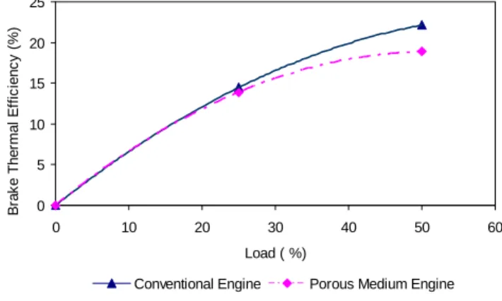
(19) A five-gas analyzer was used to measure CO, unburned hydrocarbons (UBHC) by infrared sensors and NOx by electrochemical sensors. A burette was used for measuring fuel consumption and a chrommel alumel thermocouple was used along with a digital temperature indicator for measuring the exhaust gas temperature. All tests were performed under steady state conditions. Tests were first conducted with a conventional engine to obtain the base data. Each test was repeated three times and the results of three repetitions were averaged. Under the same operating conditions, the testing was extended to the porous medium engine which was under investigation. However, the loading of engine was restricted to 50 % of peak load due to limitation imposed by the endurance strength of the porous ceramic material. The performance parameters and exhaust emissions obtained with this porous medium engine were compared with those of conventional engine.. 4. Results and discussion 4.1 Performance characteristics 4.1.1 Specific fuel consumption The presence of porous medium enforced a restriction to the intake air flow which ultimately resulted in marginally lower volumetric efficiency than the conventional engine. In turn, this caused a marginal increase in the specific fuel consumption in the case of the porous medium engine. This is shown in Figure 3. If the combustion chamber volume was maintained by some means, it was strongly anticipated that there would be negligible difference in the specific fuel consumption of conventional engine and porous medium engine.. Volume 2009-3. 0.8 0.7 0.6 0.5 0.4 0.3 0.2 0.1 0 0. 10. 20. 30. 40. 50. 60. Load ( %). Conventional Engine. Porous Medium Engine. Figure 3: The effect of porous medium on specific fuel consumption. 4.1.1 Brake thermal efficiency At light loads, the porous medium engine produced almost equal brake thermal efficiency of a conventional engine. But when the load on the engine was further increased, the porous medium engine had slightly inferior brake thermal efficiency. This is shown in Figure 4. Higher fuel consumption resulted in lower brake thermal efficiency in the case of the porous medium engine. 25 Brake Thermal Efficiency (%). engine was equipped with an orifice meter connected to an inclined manometer to measure mass flow rate of the intake air. An air damping tank was used for damping out the pulsations produced by the engine, thus obtaining a steady air flow.. Specific Fuel Consumption (g/kWh). European Journal of Mechanical and Environmental Engineering. 20 15 10 5 0 0. 10. 20. 30. 40. 50. 60. Load ( %) Conventional Engine. Porous Medium Engine. Figure 4: The effect of porous medium on brake thermal efficiency. 4.2 Emission characteristics 4.2.1 Unburned hydrocarbons The porous medium engine had superior emission characteristics when UBHC emissions were being considered. This is shown in Figure 5. In the case of porous medium engine, the UBHC were mainly eliminated by the extremely fast and complete vapourization of the fuel which was injected inside the porous medium and also due to complete combustion. The two phenomena responsible for UBHC in a conventional engine (over-mixing and under-. 19.

(20) European Journal of Mechanical and Environmental Engineering mixing) were totally eliminated in porous medium engine, since the fuel was not injected in the free space of the cylinder but inside the porous medium.. combustion heat from completely entering the combustion gases and therefore no temperature peaks occurred. This differentiated the porous medium combustion from the conventional engine combustion process. 1000. 20. 900 Oxides of Nitrogen (ppm). Unburned Hydrocarbons (ppm). 25. Volume 2009-3. 15 10 5 0 0. 10. 20. 30. 40. 50. 800 700 600 500 400 300 200 100. 60. 0. Load (%) Conventional Engine. 0. 10. 20. 30. 40. 50. 60. Load ( %). Porous Medium Engine. Figure 5: The influence of porous medium on unburned hydrocarbon emission. Conventional Engine. Porous Medium Engine. Figure 7: The influence of porous medium on nitrogen oxides emission. 4.2.2 Carbon monoxide. 0.14. 4.2.4 Soot 70 60 Soot (mg/m3). Figure 6 shows that the porous medium engine was producing low emissions of CO. This was due to the fact that, in the porous medium engine, homogeneous temperature conditions had been accomplished inside the engine cylinder throughout the combustion process. This led to unbelievable low emissions of CO in porous medium engine than a conventional engine.. 50 40 30 20 10 0 0. 0.12. 10. 20. 30. 40. 50. 60. Load (%). CO ( %). 0.1 Conventional Engine. 0.08. Porous Medium Engine. Figure 8: The influence of porous medium on soot emission. 0.06 0.04 0.02 0 0. 10. 20. 30. 40. 50. 60. Load ( %) Conventional Engine. Porous Medium Engine. Figure 6: The influence of porous medium on carbon monoxide emission. 4.2.3 Oxides of nitrogen The proper design of the porous medium engine yielded temperature-controlled combustion, which also being characterized by low NOx emissions. This was principally achieved due to the presence of solid phase of porous medium during combustion. This prevented the. From the figure 8, it was evident that soot emissions began to drop once the load on the engine had been increased. In the case of porous medium engine, the soot emission was primarily reduced by the following factors: the lower temperature in the reaction zone, very fast vapourization, more homogenous mixture composition and relatively long residence time in the reaction zone with a homogeneous temperature distribution [4].. 5. Concluding remarks The major performance and emission characteristics obtained from porous medium engine under investigation were summarized and given below.. 20.

(21) European Journal of Mechanical and Environmental Engineering. . . Reduced NOx formation due to lower temperature peaks and homogenous combustion conditions. CO and HC emissions were found to be lower than the conventional engine owing to the complete vapourization and clean combustion of fuel. Soot emission was diminished due to fast and complete vapourization and the homogeneous combustion conditions. To some extent, the porous medium engine had inferior characteristics with respect to specific fuel consumption and brake thermal efficiency, which had been imposed due to restriction to the incoming air inside the engine cylinder by the placement of porous medium. But if the air inside the engine cylinder would be maintained by some external means (supercharging or turbo charging), the porous medium was anticipated to give better results in terms of brake thermal efficiency and specific fuel consumption as well.. Volume 2009-3. [7] Miroslaw Weclas, Potential of porous medium combustion technology as applied to internal combustion engines, Sonderdrunck Schriffenreihe Der Georg-Simon-OhmFachhochschule Numberg NR.32, ISSN 1616-0762, 2004.. References [1] Miroslaw Weclas, Strategy for intelligent internal combustion engine with homogeneous combustion in cylinder, Sonderdrunck Schriffenreihe Der GeorgSimon-Ohm-Fachhochschule Numberg NR.32, ISSN 1616-0762, 2004. [2] Durst. F, Weclas, M., A new type of internal combustion engine based on the porous medium combustion technique, Proc. Instn Mech Engrs,Vol 215, Part D, pp.63-81, 2001. [3] W.G.Wang, D.W.Lyons, N.N.Clark and M.Gautam, Emissions from nine heavy trucks fueled by diesel and biodiesel blend without engine modification, Environmental Science Technology, Vol 34, pp.933-939, 2000. [4] Bone W.A., Surface Combsution, J.Franklin Inst.State Penn, 173 (2), pp.101-131,1912 [5] Macek Jan, Polasek Milos, Porous medium combustion in engines may contribute to lower NOx emissions, Joesef Bozek Research Center, Czech Technical University in Prague, Czech Republic, Paper Code: F02V147 [6] S.Afsharvahid, P.J.Ashman, B.B.Dally. Investigation of NOx conversion characteristics in a porous medium, Combustion and Flame, Vol 06, pp.112,2007. 21.

(22) European Journal of Mechanical and Environmental Engineering. Volume 2009-3. Experimental Investigation of Turbulent Heat Transfer in a Horizontal Tube with Longitudinal Strips a. S.N. Sarada, K.K. Radha , A.V.S. Raju Department of Mechanical Engineering, JNTUH College of Engineering, Kukatpally, Hyderabad-500085, Andhra Pradesh, India, Asia. Email: kalyaniradha@gmail.com. Abstract The present work shows the results of an experimental investigation of the augmentation of turbulent flow heat transfer in a horizontal tube by means of strip type inserts, with air as working fluid. Three kinds of longitudinal strip type inserts-square, rectangular and tapered strip are studied. The Reynolds number ranged from 5000 to 13000. Regression equations for friction factor and Nusselt number are developed. It is observed that the enhancement of heat transfer as compared to a conventional bare tube at the same mass flow rate was found to be a factor of 8 to 10 times for square insert, 3.5 to 4 times for rectangular insert and 7 to 8 times for tapered inserts, where as the friction factor rises was only about a factor of 1.2 times for square, 1.17 times for rectangular and 1.14 times for tapered insert.. Keywords: heat transfer, enhancement, augmentation, tapered inserts, rectangular inserts.. 1. Introduction Among many techniques (both passive and active) investigated for augmentation of heat transfer rates inside circular tubes, a wide range of inserts have been utilized, particularly when turbulent flow is considered. The inserts studied included twisted tape inserts, coil wire inserts, brush inserts, mesh inserts, strip inserts etc. Hsieh and Huang conducted experimental studies for heat transfer and pressure drop of laminar flow in horizontal tubes with/without longitudinal inserts [1]. They reported that enhancement of heat transfer as compared to a conventional bare tube at the same Reynolds number is a factor of 16 at Re≤ 4000, while a friction factor rise of only 4.5 is observed. Hsieh and Kuo [2] conducted experimental investigations for the augmentation of tube side heat transfer in a cross flow heat exchanger for turbulent flow of air by means of strip type inserts. They found that longitudinal strip inserts perform better than crossed strip (CS) and regularly interrupted strip (RIS) inserts for high Reynold numbers [2]. Bogdan I. Pavel and Abdulmajeed A. Mohamad [3] experimentally investigated the effect of metallic porous inserts in a pipe subjected to. constant and uniform heat flux at a Reynolds number range of 1000-4500. The maximum increase in the length-averaged Nusselt number of about 5.2 times in comparison with the clear flow case and a highest pressure drop of 64.8Pa were reported with a porous medium fully filling the pipe. Angirasa [4] performed experiments that proved augmentation of heat transfer by using metallic fibrous materials with two different porosities namely 97% and 93%. The experiments were carried out for different Reynolds numbers (17,000-29,000) and power inputs (3.7 and 9.2 W). The improvement in the average Nusselt number was about 3-6 times in comparison with the case when no porous material was used. Fu et al [5] experimentally demonstrated that a channel filled with high conductivity porous material subjected to oscillating flow is a new and effective method for cooling electronic devices. Betul Ayhan Sarac and Bali [6] conducted experiments to investigate heat transfer and pressure drop characteristics of a decaying swirl flow by the insertion of vortex generators in a horizontal pipe at Reynolds numbers ranging from 5000 to 30000 and observed Nusselt number increases from 18% to 163% compared to smooth pipe.. 22.

(23) European Journal of Mechanical and Environmental Engineering. Volume year - issue. Experimental investigation on heat transfer and friction factor characteristics of circular tube fitted with right-left helical screw inserts of equal length and unequal length of different twist ratios was done by Sivashanmugam and Nagarajan [7]. They observed heat transfer enhancement for right left helical screw inserts being higher than that for straight helical twist for a given twist ratio. A maximum performance ratio of 2.97 was obtained by helical screw inserts. Heat transfer, friction factor and enhancement efficiency characteristics in a circular tube fitted with conical ring turbulators and a twisted-tape swirl generator were investigated experimentally by Promvonge and Eiamsa-ard [8]. Air was used as test fluid. Reynolds number varied from 6000 to 26000. The average heat transfer rates from using both the conical-ring and twisted tape for twist ratios 3.75 and 7.5 respectively are found to be 367% and 350% over the plain tube. The effect of twotube inserts wire coil and wire mesh on the heat transfer enhancement, pressure drop and mineral salts fouling mitigation in tube of a heat exchanger were investigated experimentally by H. Pahlavanzadeh et al [9] with water as working fluid. The heat transfer rate averagely increased by 22-28% for wire coil and 163174% for wire mesh over a plain tube value depending on the type of tube insert, density of wire torsion and flow velocity. Pressure drop also increased substantially by 46% for wire coil and 500% for wire mesh.. air. The test pipe is connected with an orifice meter to measure the flow rate of air through the pipe. Input to heater is given through a dimmer stat. The test tube is made of a copper tube with inside diameter of 27.5 mm. A heat generating element is wound around this test tube so that the required heat input is given. The thermocouples were installed to measure the test tube wall temperature. The display unit consists of a voltmeter, an ammeter, a dimmer stat, and a temperature indicator. Heat input can be varied by changing the voltage and current which are in turn altered by the dimmer stat. The circuit was designed for a load voltage of 0-220 V, with a maximum current of 10A. Outlet of the test pipe section is connected to the orifice meter and a Utube water manometer.. Previous studies have not addressed heat transfer in tubes with tapered inserts through the range of turbulent flow regime. Hence the present study attempts to experimentally investigate the friction and heat transfer characteristics of air flowing through a horizontal circular tube with tapered inserts along with square and rectangular inserts.. The fluid properties were calculated as the average between the inlet and outlet bulk temperature. Usually, it takes 90 min. to reach steady state. Experiments are done at constant heat flux condition. For this purpose, at different heat inputs and different mass flow rates, the experiment is done with and without inserts, assuming the air flowing through the circular tube to be hydro dynamically and thermally fully developed turbulent flow. The experiment is carried out using square, rectangular and tapered inserts (Aluminium).. 2. Experimental Layout and Procedure Figure 1 shows the experimental layout consisting of an air blower, a test pipe section, a display unit, thermocouples, an orifice meter, a manometer and a flow control valve. The blower is connected to the test section (horizontal pipe). A Nichrome bend heater encloses the test section to a length of 40cm. Four thermocouples are embedded on the wall of the tube and two thermocouples are placed in the air stream one at the entrance and another at the exit of the test section to measure the temperature of flowing. Figure 1: Line diagram of the Experimental layout. 2.1 Sequence of Operation Experiments are carried out for two situations, i.e. with insert & without inserts inside the pipe section. The inserts are • Square insert (Aspect Ratio A.R=1) • Rectangular insert with A.R = 2.5 • Taper insert case-I • Taper insert case-II (With A.R = 1 at one end to A.R=2.5 at other end). 23.

(24) European Journal of Mechanical and Environmental Engineering. Without insert (Plain Tube Experiment): Experiments were conducted for 3, 4 and 5.4 inches of water level difference in manometer by varying heat inputs 40 W and 60 W. The Nusselt number obtained from experimental data is compared with the one obtained by using the Dittus-Boelter equation. The experimental uncertainity is observed to be 8%. With insert (Square,Rectangular and Tapered) It is taken care of that the strip doesn’t get corrugated at the inner walls of the pipe while inserting as shown in Figure 2. Due to the presence of the straight tape inside the tube, the flow region gets bifurcated and so there is formation of two sub–boundary layers compared to the previous case where there is no insert. The insert acts as an obstacle and due to its presence there is haphazard motion of the fluid particles resulting in turbulence. The hydraulic diameter of the square insert is diminutive in contrast to bare tube due to which the bulk temperature as well as surface temperature are significantly high in the insert which indicate the increase in heat transfer rate. After estimating the heat transfer coefficients by the energy balance equation, a correlation is developed between the Nusselt number and Reynolds number. The value of the Nusselt number obtained from the present experiments is compared with the value obtained by previous researchers (Shou-Shing Hisen, Feng-Yu Wu, Haung-Hsiu Tsai). The deviation is observed to be 8%.. Volume year - issue. In this case, highly restricted end is placed at the beginning of the test tube. The local Nusselt number and Reynolds number are estimated at different cross-sections along the length. It is observed that Reynolds number and friction factor increase along the length but the local Nusselt number decreases. It is know that as aspect ratio decreases Nusselt number must increase as they are inversely related. This contradiction is observed because there is a high restriction for the air at the entrance. After deflection at the beginning air is bifurcated into two parts with increasing aspect ratio along the test tube without making any contact with the insert i.e. behind the larger end. Case(I):. Figure 3: Fully developed turbulent flow in pipe with longitudinal tapered insert To get an optimistic result, we have reversed the above arrangement as shown below. Case (II): In this case, restriction increases slowly along the length as shown in Figure 4. Thermal properties such as local Nusselt number and friction factor are estimated at each cross section along with local Reynolds number. It is observed that local Nusselt number and Reynolds number decrease with increasing aspect ratio and friction factor increases along the length as restriction increases slowly.. Figure 2: Fully developed turbulent flow in pipe with longitudinal insert. 2.2 Longitudinal Tapered Insert The aluminium strip is tapered uniformly along its length with one end diagonal equal to the diameter of the pipe which forms a tight fit with the test tube. The other end is supported on the needles with holes drilled on both faces of the strip, so that strip is centrally aligned with the test tube. The experiment is carried with two tapered strips and is shown in the Figure 3.. Figure 4: Fully developed turbulent flow in pipe with longitudinal tapered insert. 3. Results and Discussions A correlation is developed between the average experimental Nusselt number estimated by using the energy balance equation and the Reynolds number and it is observed that the average Nusselt value of tapered insert lies between that of a square and rectangular insert and the friction. 24.

(25) European Journal of Mechanical and Environmental Engineering factor is less than the rectangular insert. By this, we can recommend that it is a good geometric shape to enhance the net heat transfer rate and to give optimum pressure drop. Table 1 shows the dimensions of tapered inserts and table 2 shows the comparison of pressure drop for different types of inserts.. L (m). W (mm). A.R. v (m/s). Nu. (hexp) 2 (W/m K). 0.15. 13.34. 1.3. 11.3. 8071. 186. 394.9201. 0.25. 15.0. 1.5. 11.7. 7884. 122. 274.4616. 0.35. 16.67. 1.6. 12.1. 7725. 76.4. 187.2610. Re. Tapered insert. Volume year - issue (case-II):. Figure 5: Variation of Nusselt number with Aspect Ratio. Table 1. shows the width of tapered inserts at different locations along the length for thickness 10 mm Type of experiment. Friction factor Pressure (f)*10-3 drop(∆p),N/m2. Plain tube. 7.984760348. 6.4098358. Square insert. 8.772981317. 235.03574. Rectangular Insert. 8.657440672. 69.702781. Tapered insert. 8.407517265. 12.342928. Table 2. shows the comparison of pressure drop along the length The maximum uncertainty between the experimental and theoretical is about 8%. A general correction for Nu and f of Re, Dh, and AR (Aspect ratio) was developed for inserted tubes using a composite power law curve fit as shown in Figures 5,6,7,8,9,10 and 11. The following graph presents the Nu and f correlated with the relevant parameter such as Re, Dh/l, and AR. The influence on Nu with Re, Dh/l, and AR are quite significant as noted the magnitude of the power dependence. The increase Re, Dh/l would result in a Nu increase. However, Nu decreases as AR increases. The case is reversed with the friction factor.. Figure 6: Variation of Nusselt number with Reynolds Number The developed correlation for Nusselt number and friction factor in terms of Reynolds number, aspect ratio and (Dh/l) for taper insert is. Nu = 0.0976 Re 0.8 AR −0.03463 (D h / l) 0.0034. (1). f = 0.0197. Re −0.0961 AR 0.0214 (D h / l) −0.0021 (2). 25.

(26) European Journal of Mechanical and Environmental Engineering. Volume year - issue. Figure 7: Variation of Nusselt number with Dh/l. Figure 10: Variation of Friction factor with Dh/l. Figure 8: Variation of Friction factor with Reynolds Number. Figure 11: shows the developed correlation for friction factor in terms of Reynolds Number, aspect ratio and (Dh/l). Figure 9: Variation of Friction factor with A.R. Figure 12: Variation of Nusselt No with mass flow rate. 26.