Male and Female Work Histories and Family Disruption in Canada

(1)

99-08

MALE AND FEMALE WORK HISTORIES AND FAMILY DISRUPTION IN CANADA Ghyslaine NEILL et Céline LE BOURDAIS

INRS-Urbanisation

Mai 1999 3465, rue Durocher Montréal, Québec

(2)

(3)

Preliminary version*

MALE AND FEMALE WORK HISTORIES AND

FAMILY DISRUPTION IN CANADA

Ghyslaine NEILL and Céline LE BOURDAIS

Paper presented in the session of Research Committee 41, “Selected Topics in Demography: III”

At the XIVth World Congress of Sociology Montreal, July 26 - August 1, 1998

Support for this research was provided by grants from the Social Sciences and Humanities Research Council of Canada (SSHRCC), the Fonds pour la Formation des chercheurs et l’aide à la Recherche (FCAR), and the Conseil québécois de la recherche sociale (CQRS). The authors wish to acknowledge the assistance of Nathalie Vachon for the preparation of the data.

* Not to be quoted without the permission of the authors.

(4)

(5)

I

NTRODUCTION

In Canada, as in most industrialized societies, union and fertility behavior has changed considerably over the last 20 years. Legal marriage has lost ground to cohabitation and marriage is no longer a necessary condition to start family life. Between 1990 and 1994, for example, 57% of the Canadians who entered their first union chose cohabitation compared to 15% of those who did so in the early 1970s, and this proportion has reached 80% in Québec (Dumas & Bélanger, 1997). The percentage of births occurring outside of marriage has risen from 13% in 1980 to 30% in 1994 (Dumas & Bélanger, 1997), and over 50% of first births are now occurring to cohabiting parents in Québec (Duchesne, 1996),

The restructuring of the economy has also affected Canadian families. As compared to the 1960s, most families can no longer support themselves on one income. Research has shown that 65% of all two parents' families were dual earner families in 1991 as compared to 20% in 1961 (Duxbury, Higgins & Lee, 1994). Furthermore, the recent increase in jobs has mainly occurred in the service sector that is linked to low-paid jobs, flexible employment and lack of union protection (Baker & Lero, 1996). As fewer people can expect to work with the same employer through their working lives, a rising percentage of couples are bound to experience periods of unemployment and underemployment.

What do those new patterns of family formation and labor force participation mean for the stability of family? In order to answer this question, we will examine separately for men and women the factors affecting the risk of family disruption from the moment a first child is born to the couple. Drawing on the retrospective data on family collected by the 1995 General Social Survey, we will analyze, more specifically, the effect that labor market related characteristics exert on the likelihood of family disruption, when controlling for the circumstances surrounding the formation of the family.

F

ROM MARRIED TO COHABITING COUPLES1

Research pertaining to union dissolution has shown that cohabiting unions are less stable than marriages (Burch & Madan, 1986; Schoen, 1992; Balakrishnan, Lapierre-Adamcyk & Krotki, 1993; Le Bourdais & Marcil-Gratton, 1996). Even for cohabitors who chose to marry, their union has been shown to be at greater risk of dissolution (Hall & Zhao, 1995; DeMaris & Rao, 1992). In terms of values and attitudes, these results suggest that cohabiting unions are selective in that the couples involved are more willing to accept separation or divorce in case of conflict (Axinn & Thornton, 1992). Recent research, however, has questioned the capability of the selectivity

1

(6)

hypothesis to account for the higher instability observed among couples who married after cohabiting, and has hypothesized that the nature of the relationship itself (e.g. the lower level of commitment of common-law partners toward the relationship and their lower level of satisfaction) plays an important role (Nock, 1995). However, is it logical to compare marriages and cohabiting unions, irrespective of their ordering within the life course of individuals, when the latter is now said to be equivalent to “going steady” 30 years ago (Nock, 1995) or to be part of the changing nature of the courtship process (Oppenheimer, 1994)?

To move the focus toward a more meaningful comparison, we decided to examine the risk of separation among different types of union from the moment a first child is born (or adopted) to the couple. By including only these unions, we are comparing couples who, at some point, have made a commitment to their relationship. In fact, studies have found that the presence of children reduces the risk of conjugal disruption for married as well as for cohabiting couples (Lillard & Waite, 1993; Wu, 1995: Wu & Balakrishnan, 1995). In both cases, the results suggest that children increase the “costs of disruption”, and that is the reason why their presence would have a positive impact on the stability of the relationship. Comparing cohabiting and married couples, Nock (1995:67) considers the “exit costs” from a union as a measure of commitment, and concludes that “because cohabitation is constrained by fewer social and legal rules than marriage”, the exit costs from a cohabiting relationship should be “less than those associated with marriage”. But, since the presence of children has been shown to have a positive impact on the existing relations between adult children and their parents, giving birth to a child should reinforce family support and thus union stability, no matter the type of union chosen.

In Canada, and especially in Québec, research has revealed that the proportion of couples who start their family in a cohabiting union has increased significantly during the 1980s. Indeed, 30% of all the births registered in Canada in 1994 were to unwed mothers, and this proportion has reached 48% in Québec (Dumas & Bélanger, 1997). Considering that births to cohabiting couples account for most of the trend observed, it is clear that family studies can no longer focus exclusively on marriage and need to take cohabitation into consideration (Bumpass & Raley, 1995; Le Bourdais & Marcil-Gratton, 1996).

Recent research has also shown that family disruption patterns among couples who married their cohabiting partners during the 1980s have become closer to those of couples who married directly than those of cohabitors (Desrosiers & Le Bourdais, 1996). Could this mean that the selectivity effect is no longer operating among younger generations? Furthermore, could we expect that the new families formed within the context of a cohabiting union in the future would tend to resemble those created directly within marriage? These questions still remain to be answered. But the diversity of paths

(7)

taken by families recently formed needs to be considered if we are to better understand the determinants of family disruption.

F

AMILY STABILITY IN A CHANGING LABOR MARKET

A large body of research has examined the effect of demographic and socioeconomic characteristics on marital disruption (Bumpass, Martin & Sweet, 1991; Cherlin, 1992; Tzeng and Mare, 1995). Paralleling the changes observed in the sexual division of labor, the rise of marital instability has since long been associated with the increase of married women’s labor force participation (for a review, see Ruggles, 1997). Consequently, most studies analyzing marital disruption have focused upon variables related to women’s work situation (employment status, number of hours worked per week, income level) and still continue to do so. But many of these studies measure women’s participation in the labor market at a single time, usually at the beginning of the marriage, and thus fail to capture the dynamic process occurring (for a critique of such studies, see Greenstein, 1990; Tzeng & Mare, 1995).

Recent analyses based on longitudinal micro-level data have challenged the idea of a fixed relationship between rising marital instability and the increase of women’s employment per se. Using panel data from the National Longitudinal Surveys of Young Women, Young Men and Youth (NLSY), Tzeng and Mare (1995), for example, developed an approach focusing upon the changes that women undergo in the labor market and in relation to their spouse. Their research suggests that both men’s and women’s work experiences strengthen marital stability, but that positive changes in wives’ socioeconomic and labor market characteristics (such as an increase in the number of hours worked) over the course of their marriage would increase the odds of marital disruption.

The relationship that has been observed between women’s work and family disruption in previous studies might have changed over time due to the changes noted in the educational attainment and employment characteristics of both young men and women. In this perspective, the improvement of women’s education might have altered the relationship observed between education and union dissolution. South and Spitze (1986) have shown that wife’s education reduces the risk of divorce in shorter marriages but increased it in longer ones; Hoem (1997) has found that the risk of family disruption for highly educated women during the 1980s increased much less than those of others in Sweden; Dharmalingam et al (1998) have found that university educated women in New Zealand are less likely to experience marital disruption than those with no qualification.

In comparison to the attention given to the impact of women’s work on union dissolution, the changing position of men in the labor market has attracted very little interest. Focusing on marriage timing, Oppenheimer et al. (1997) have looked at the

(8)

changes that young men are experiencing in the labor market aiming to account for delayed marriage. Their findings suggest that marriage formation among young men be closely related to career development: the more difficult it is to establish a career, the longer marriage will be delayed.

In a context where the ability to establish and maintain an independent household above some socially acceptable minimum level is strongly related to young couples market position (op. cit.), men’s economic characteristics have to be considered when studying family disruption. As shown by Oppenheimer (1994), the employment situation of young men with a high school degree or less has considerably deteriorated since the 1970s in United States. If moderately or less educated young men are more affected by unemployment, underemployment or “short-time” jobs, what does it mean for the stability of their family? Are unions in which the male partners do not have at least a college degree today more at risk of separation? Moreover, are men not steadily employed more likely to experience family disruption?

In this paper, we compare men and women risk of family disruption taking into consideration the effect of their changing position in the labor market as well as the circumstances surrounding the formation of their respective family. Following the description of the data, measures and the methodology used, we present the results for women first and then for men. Considering the approach taken in recent research, we will try to refine our measure of labor force participation by using various indicators of the respondents’ movements in and out of the labor force. In order to examine the extent to which the effect of education have changed over time, the interaction between education and birth cohort will be tested for both men and women.

D

ATA AND METHODOLOGY

Data

The data used in this paper come from the General Social Survey (GSS) on Family (cycle 10) carried out by Statistics Canada during 1995. The GSS is a stratified sample of 10,749 individuals aged 15 years and over living in Canada in 19952; of these, 5,914 were women and 4,835 were men. The GSS collected detailed retrospective data on the conjugal (marriages and cohabiting unions), parental (children born to or raised by respondents) and work (employment and job interruptions) histories of all respon-dents, in addition to respondents’ current characteristics at the time of the survey (Statistics Canada, 1997).

2

(9)

The conjugal histories gather information on the timing of entry into and exit from all marriages and cohabiting unions that respondents have experienced through the course of their life; for each of these unions, we know the circumstances (separation, divorce, death of partner) surrounding its dissolution, where applicable. The parental histories provide data for all the children born to or raised by the respondents (biological, adopted or stepchildren): for all these children, we know the date of birth3, and for adopted or stepchildren, we also know the date of the children’s arrival into the respondents’ household. With these data, we were able to identify the union, in which respondents had or adopted their first child, and to follow the unfolding history of their family. Respondents who had their first biological child outside of a union, as well as those who started their parental career as a stepparent of their partner’s children were excluded from our analysis. The rationale for doing so is based on previous research that has shown that step-families formed after separation or following the birth of a child outside of a union4 (marriage or cohabitation) face additional difficulties (such as the lack of institutional norms to guide step-parents’ behaviors) over and above those experienced by intact families, and greater risks of union dissolution (Cherlin, 1992). Following this strategy, we identified 1,774 female and 1512 male respondents who gave birth to their first child while living in couple between 1970 and 19955; women were aged between 25 and 64 years and men between 25 and 69 years at the time of the survey. 510 women and 316 men had experienced a separation when they were reached by the GSS in 1995.

Indicators of the Conjugal Circumstances Surrounding the Formation of

the Family

Conjugal Sequence Followed - To investigate the effect that the conjugal path followed by parents exerts on the risk of union dissolution, we distinguished three categories of respondents, that are entered into the analysis as dummy variables: 1) those who married directly prior to the birth of the child; 2) those who were still cohabiting when the child was born; and 3) those who married their cohabiting partner before having a child (for respondents’ distribution, see Table 1). A fraction of the latter

3

In fact, the public microdata file provides the age (in decimal form) of respondents at each event: union formation and dissolution, birth or adoption of the child, etc.

4

A single-parent family created by the birth fo a child outside a union may lead to the formation of an intact family if the two biological parents start living together, or of a step-family if, for instance, the single parent enters a union with a partner who is not the biological parent of the child. The GSS contains no information on the conjugal and parental status of the respondents’ partners and thus, does not allow us to distinguish among these two types of family. Based on previous work, we assumed that single parent who started living with a partner less than six months after the birth of their child did so with the biological parent of their child; they were thus included in our analysis.

5

Families formed before 1970 were excluded from the analysis because the development of cohabitation and the rise of divorce appeared mostly during the 1970s.

(10)

will eventually marry along the road, and some of them had probably already planned to do so when their first child arrived. In order to take into account those cohabiting unions that are legalized through marriage, we created time-varying covariates for the last two categories. In other words, respondents who were still cohabiting at the birth of their first child were first given a value of 1 on the second dummy variable and a value of 0 on the other two dummies: from the moment they marry, the third dummy (marrying after cohabiting) takes the value of 1, while the other two are set to 0.

Birth Cohort - We introduced a cohort variable to control for the changing context in which individuals formed their families. We distinguished respondents born during the 1960s, the 1950s and before the 1950s. Most of respondents born before the 1950s formed their families within a marriage while the respondents born during the 1950s or the 1960s did so in a context characterized by the rise of divorce and the development of cohabitation.

Indicators of Socioeconomic Characteristics

Labor Force Attachment - The retrospective data collected on work histories gather information on jobs and work interruptions that lasted at least six months while respondents were not attending school full-time. For those who worked at a job or business for at least six months, either part-time or full-time, we know the age they had at the beginning of the job. For respondents who stopped working for a period of six months or longer, we know their age (in decimal form) when they quitted the labor market, and the duration (in months) of their work interruption. These data are available for up to five jobs and four interruptions. Approximately 92% of women and 99% of men were employed on a regular basis at some point before or during the family episode.

In order to examine the attachment of men and women to the labor market, we developed a series of indicators (time-varying covariates). These indicators aim to trace their movements in and out of the labor market and to take into account the cumulative effects that either continuous employment or repeated work interruptions might exert on their propensity to experience family disruption. Our strategy thus focuses on the changes that respondent's experience on the labor market, and those time-varying variables can reflect these changes.

The first time-varying covariate we developed specifies whether or not respondents were employed from the moment they had their first child up until the separation or the survey if they were still living in couple. This time-varying dummy is coded 1 for each duration (measured in tenths of a year) of the family in which the respondent is employed, and 0 for each duration during which she or he has stopped working. The second time-varying covariate is a cumulative variable that measures the number of years (in decimal form) that respondents spent on the labor market. It starts

(11)

with the number of years of work experience that a person has accumulated at family formation (e.g. at the birth of the first child), and this number increases continuously with her or his presence in the labor market. The third time-varying covariate is also a cumulative variable that counts the number of work interruptions experienced by men and women from the moment they started to work on a regular basis up to the separation of the couple or to the time of the survey. In order to take into consideration the period at entering work on a regular basis, we created a last time varying covariate. Five categories are distinguished and entered as dummy variables into the equation:

1) never worked;

2) entered employment before 1970; 3) between 1970-79;

4) between 1980-89; and 5) between 1990-95.

Respondents who started to work after family formation were given a value of 1 on the first dummy variable (i.e. never worked) and a value of 0 on the other four dummies; from the moment they started working, the dummy corresponding to the job entry into the labor market takes the value of 1 while the others are set to 0.

Educational Attainment and Time Out of School - The GSS provides information on the level of education attained at the time of the survey and on the age at which respondents completed their studies. Having no information on the level of schooling completed by respondents when they first entered a union or had their first child, we were forced to use the level attained at the moment of the survey, as a proxy of educational attainment6. However, in order to take into account the impact that the sequencing of events has on the propensity of respondents to go through a family disruption, we created a dummy variable that measures whether or not a man or a woman had completed their schooling when they formed the union in which they bore their first child. Approximately three respondents out of ten had not completed their studies when they started living with their partner (Table 1).

To explore the extent to which the effect of education have changed over time and, then might affect differently the risk of going through family disruption, we also tested for interactions between education and birth cohorts.

Other Variables - In addition to the circumstances surrounding the formation of the family and to the work and educational characteristics discussed above, we also examined the effects of other covariates that are likely to affect family disruption. We

6

The GSS collected the number of years of elementary and high school education completed (up to thirteen years), and the highest level (in terms of diploma) of education achieved past high school. We thus had no other choice than to use dummies to measure educational level attained at the time of the survey.

(12)

included the age of the respondents at the beginning of the family episode, which is entered as a dummy variable into the model, and we controlled for whether or not the child was conceived before the couple had married or started to cohabit7. Roughly, one respondent out of ten had conceived their first child prior to union formation (Table 1).

Finally, we introduced the region of residence at the time of the survey to distinguish respondents living in the province of Québec from those living in the rest of Canada (Table 1). This should allow us to see if the rapidly changing pattern of family formation in Québec has any impact on family disruption as the majority of young adults favor cohabitation over marriage as they enter their first union and start their family.

Statistical Methods

We use proportional hazards models to study the process of union dissolution among intact families (see Allison, 1984). The dependent variable in the models is the instantaneous rate of union dissolution experienced by men and women living in those families, and it is expressed as a function of two components: an underlying or baseline function, which varies over time but whose form is left unspecified, and the effects on this baseline hazard of a set of individual characteristics, some of which may change over time (Cox, 1972). Here, it is important to recall that the risk of union dissolution is estimated from the moment a child is born to the couple and not from the beginning of the union. The independent variables include the fixed and time-varying covariates described above. Several nested models were estimated in order to examine how the progressive addition of each covariate mitigates or reinforces the effect of the others. However, only the complete models are shown here.

The parameter estimates are presented in their exponential form and thus express the hazard of a specific group as a proportion of the baseline hazard. A coefficient greater than 1 indicates that the characteristic analyzed increases the chances of respondent to experience a union dissolution, while one smaller than 1 reveals that it reduces that risk. Many of the covariates are entered into the equations as dummy variables, and the coefficients presented in table 2 thus need to be interpreted in relation to the reference category (given in parentheses). For continuous variables, the coefficients express the increase (or decrease) in the risk of respondents to go through family disruption for each increase of one unit on the metric variable. The final sample8 consists of 1,542 female respondents and 1,347 male respondents who formed their

7

We considered as pre-union conception all births that occurred 0.7 year (i.e. 8.4 months) or less after the beginning of the union.

8

(13)

family after 1969, and for whom it was possible to reconstruct their family and work histories and for whom no data is missing9.

R

ESULTS

All women

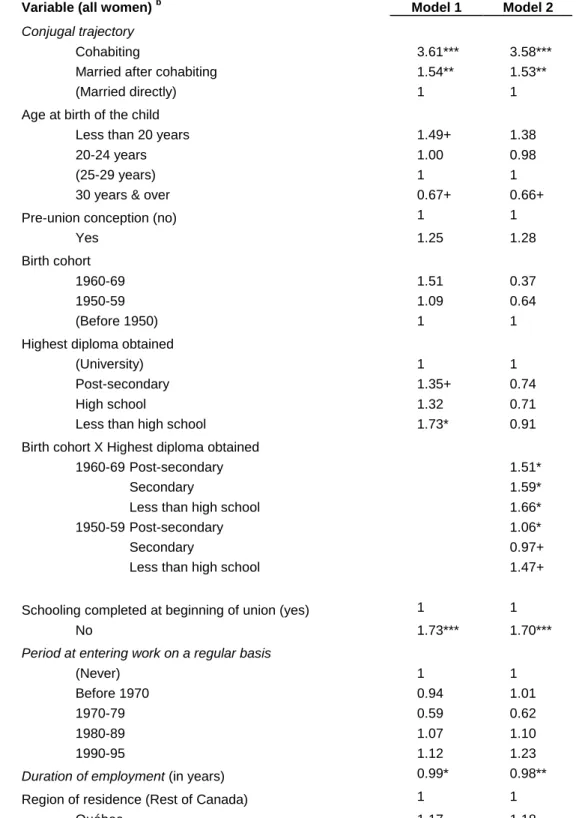
Two models are presented in Table 2. The first examines the effects that the basic covariates exert on the likelihood of all women irrespective of their work history -to experience family disruption, while the second model tests more specifically for the interaction between education and birth cohort. As found in other studies, the type of union chosen at family formation has a strong influence on the risk of union breakdown. Women who were cohabiting and continue to do so later on have approximately three and a half times more chances to separate than those who married directly before entering family life. Women who married their cohabiting partner have about 50% more chances to experience union dissolution (see Model 1, Table 2). Age at family formation also affects the propensity of women to experience union dissolution: compared to those who were aged between 25 and 29 years old at the birth (or adoption) of first child, younger women have 49% more chances to experience family disruption while women aged 30 years and over have 33% less chances to do so. Pre-union conception is also linked to a higher probability of family disruption although the effect is not statistically significant. The same comment applies to birth cohort: women born between 1960 and 1969 have 51% more chances to experience family disruption when compared to women born before 1950, but the coefficient is not significant.

The level of schooling completed at the time of the survey exerts a negative effect on family disruption: when compared to women who hold a university diploma, women who have completed less than high school have 73% more chances to experience a union breakdown, while women with a post-secondary education have 35% more chances. The coefficient obtained for women with a high school diploma, although not significant, indicates a higher propensity to separate. Irrespective of the diploma obtained, women who had not completed their studies when entering the union in which they started their family face a greater risk (1.73) to go through a union dissolution that those who had completed their schooling.

Even if coefficients obtained for the period at entering work on a regular basis are not significant, they are indicating different patterns of labor force participation when we

9

196 (unweighted) female and 165 (unweighted) male cases were excluded from the analysis because of missing data in the education or work histories. In order to check for the possible biases induced by the elimination of these cases, we compared the coefficients associated with all covariates except for the work related variables. When including and excluding these cases from the model we observed no significant differences between the two sets of coefficients.

(14)

compare women who worked on a regular basis to those who never did. When controlling for all the covariates retained in the analysis, and thus for birth cohort, women who entered work before the 1980s, and especially between 1970 and 1979, have less chances of experiencing family disruption than those who never worked. After 1980, women who entered labor force have more chances when compared to the one who never did. This might be explained by the new patterns of labor force participation in recent years where women do not go out of the labor market when entering motherhood. If the period at entering work on a regular basis is not significant; the cumulative experience of women on the labor market appears to be affecting significantly their propensity of experiencing family disruption. Our result shows that duration of employment reduces the risk of union dissolution, result that supports the idea that the impact of women’s work might have changed over time.

Finally, the region of residence at the time of the survey does not appear to significantly influence the risk for a woman to experience family disruption when controlling for all the covariates in the model.

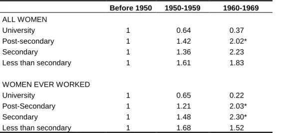
When the interactions terms between education and birth cohort (table 2 model 2) are introduced into the equation, the size of the coefficients of the remaining covariates is not modified significantly (except for those related to the interaction terms). The interaction terms are significant but are difficult to interpret directly. To gain a better understanding of how they operate, we decided to compare first, how the effect associated with each level of education has changed through time (upper panel of table 4), and second, how the effect associated with each cohort varies according to the level of education completed (lower panel of table 4).

Looking at results for all women, we found that chances to go through a union dissolution increases over time for all levels of education completed, except for university degree to which the propensity to separate decreases with time (but coefficient is not significant). When compared to women with a post-secondary diploma, those born between 1960 and 1969 are at greater risk of family disruption than those bore earlier (2.02). If we now look at how changes in levels of education affect the propensity to separate within each birth cohorts, we find that holding a university diploma reduces considerably the risk of family disruption for women who were born between 1960 and 1969 and to a lower extent for those born in the 1950s. For those who hold a post-secondary diploma, the risk of union dissolution increases considerably: women who were born between 1950 and 1959 have 65% more chances to go through a family breakup while the risk for those born in the 1960s are more than four times higher.

Those results suggest that the propensity to go through a union dissolution has increased across generation except for those who hold a university diploma. Holding a university diploma seems to have a protective effect against family disruption (when controlling for age at birth or adoption of the first child). But, how much of what has been

(15)

observed is linked to the fact that women with a university degree have better job prospects than their less educated counterparts? In the following section, we attempt to answer this question by focusing our analysis on women who have worked on a regular basis before or during family episode.

Women who ever worked

In order to assess the impact of women’s continuity/discontinuity into employ-ment on the chances to experience family disruption, we have excluded from the analysis women who never entered work on a regular basis. This strategy left us with a sub-sample of women (1445) who worked on a regular basis before or during the family episode (see Table 1). As in Table 2, Table 3 presents two models. The first one examines the effects that all covariates10 exert on the likelihood to experience family disruption, and in the second one, we are testing for the interaction between education and birth cohort.

When compared to the entire sample of women, the impact exerted by the type of union, the birth cohort and the highest diploma obtained on the likelihood of family disruption for the sub-sample remains similar. However, the effect of age at family formation is slightly modified: except for women who started their family at age 30 or older who still face lower chances of experiencing family disruption than those aged between 25 and 29, no significant differences separates women who had their first child at a younger age. The impact of pre-union conception turns out to be more important in increasing the risk of separation. The size of the coefficients for birth cohort and highest diploma obtained are also the same although it becomes significant at .10 for younger women (1.48+). Finally, the completion of schooling at union formation remains strongly significant, as the risks are 61% higher for women who were not finished.

For women who ever worked, the fact of being employed at any time during the family episode increases significantly the risk of union breakdown. Compared to women who are not employed, those holding a job are approximately five times and a half more likely to experience separation. This result support the idea that when women are currently working, they are more at risk of separation because of the existence of stress or conflicts associated with the multiple roles to be performed (worker, spouse, and parent) (Duxburry, Higgins & Lee, 1994). Our results also show that the stronger is the attachment of a woman to the labor market the higher is her propensity to experience union dissolution: hence, cumulative duration of employment appears to be positively

10

The period at entering work on a regular basis has been excluded from this model while two other time-varying variables have been included i.e. employed or not during family episode and the number of work interruptions.

(16)

linked to the risk of facing family disruption. The cumulative number of work interruptions does however, appear to increase the risk of union dissolution, although not significantly. As we did for the entire sample of women, we also included interaction terms between birth cohort and highest diploma obtained in our analysis of women who have ever been employed on a regular basis (Table 3 model 2). We found the size of the coefficients to be the same for all covariates, except the variables included in the interaction terms. The results obtained are in the same lines that the ones obtained for the entire sample of women: for women born before 1950, having a university diploma leads to greater risk of family disruption, although the coefficients obtained are not significant. If we compare women who have a university diploma, we find those born before 1950 to be at greater risk when compared to the other birth cohorts.

A specific analysis of the interaction between education and birth cohort (Table 4) for women who ever worked support, once more, the idea that the impact of education changes over time. When comparing the risk of family disruption for women with a university diploma, we find that those born before 1950, present higher risks but the coefficients are not significant. For women with a post-secondary or a secondary diploma and who were born between 1960 and 1969 they are at greater risk of family breakdown (respectively 2.03* and 2.30*).

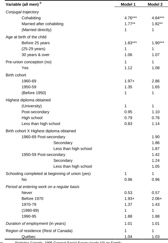
All men

The same type of analysis has been applied to men and results are presented in tables 5 to 7. Table 5 presents two models: as for women, the first examines the effects that all covariates exert on the likelihood of all men to experience family disruption, and the second model is testing for the interaction between education and birth cohort. As it has been observed for women, the type of union chosen at family formation has a strong influence on the risk of union dissolution. Men who were cohabiting and continue to do so during the family episode have over four times and an half more chances to separate than those who married directly before entering fatherhood; and men who married their cohabiting partner have 77% more chances to do so. Men’s age at family formation also affect very strongly their propensity to experience union dissolution: compared to those who were aged between 25 and 29 years old, men who became father before 25 years of age have 83% more chances to experience family disruption. The link between pre-union conception and family disruption is positive but not significant for men as it was for women (1.12 and 1.25). Men’s birth cohort appears to be related to family disruption, with younger men having close to twice as many chances to go through a union breakdown than men born before 1950.

Unlike women, the level of education completed by men does not appear to significantly affect their propensity to separate, once controlling for the variables included

(17)

in the model. The period in that men started working on a regular basis do, however, influence there chances to experience family disruption.

As compared to the analysis conducted for women, we changed, here, the reference category of this variable, since the number of men who never worked before or during family episode is very small (20 unweighted cases). Even when controlling for covariates such as birth cohort and age at birth at family formation, men who entered work on a regular basis before 1970 have 93% more chances to have a union breakdown than those who did so between 1980 and 1989. Unlike women, the cumulative duration of employment has no impact on the risk of family disruption.

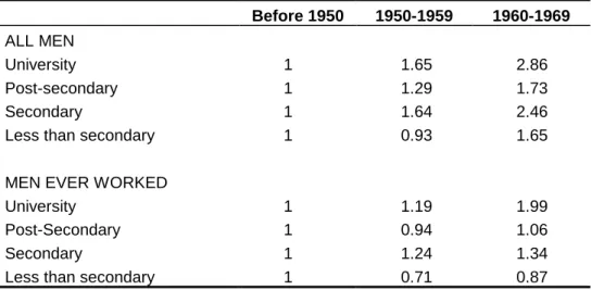
The inclusion of the interactions terms between education and birth cohort (table 5 model 2) does not modify significantly the size of the coefficients of any of the covariates included in the model, except for those related to the interaction terms. As opposed to women, none of the interaction coefficients turn out to be significant. But, if we compare the results to those obtained for women, they are quite different if not completely at the opposite. A university diploma put men at greater risk of family disruption for each birth cohort while younger men with a university degree, when compared to the older ones, seems to be worst off.

Men who ever worked

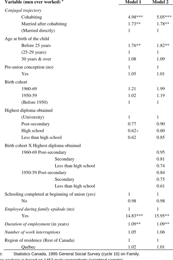
The results shown in table 6 excludes men who never worked before or during family episode, as we want to evaluate more closely the impact of their position in the labor force on their chances to separate. As in the previous analysis, the first model presents all covariates without the interaction between birth cohort and education, while the second one integrate them. The impact of the type of union and of the age at birth of first child on the likelihood of family disruption remains similar to that observed for the whole sample. But, the exclusion from the analysis of men who never worked modifies the coefficient associated to the birth cohort: men born in the 1960s then no longer faces a higher propensity to separate than those born before 1950.

As for women, we found that being currently employed at any time during the family episode and from the moment the first child is born (or adopted), increases significantly the men’s risk of union breakdown. Compared to those who are not employed, men who are have almost 15 times more chances to experience separation. Our results also show that the longer the duration of employment, the higher is the men’s propensity to experience union dissolution. Finally, the risk of separation appears to be growing with the cumulative number of work interruptions, although the coefficient is not significant.

(18)

When including the interaction terms in the analysis (table 6 model 2), the size of the coefficients obtained for all covariates remains similar except for those related to the interaction terms, and none of the results shown in table 7 are significant.

D

ISCUSSION

This study has shown that the type of union chosen by men and women at family formation has a considerable impact on the risks of separation. Consistent with previous research, we found that male and female respondents who were in a cohabiting relationship exhibit higher risks than those who married directly. But, the ones who chose to marry after cohabiting have fewer chances to separate than those who maintained their cohabiting relationship. Age at family formation has a much bigger impact on men than women. Indeed, having a first child before the age of 25 increases young men’s risks of union dissolution. Concerning pre-union conception or region of residence, we have not seen any significant impact for men and women as well.

Our results have also shown that the effect of women’s education has changed over time. If we analyze those results in light of the trends observed in women’s labor force participation, we can start to understand why the same diploma has a different impact across birth cohort. Highly educated women have always participated to the labor market. But, in a context in which women used to stop working when entering motherhood, the pursuit of a career could bring additional family tensions and lead eventually to a separation. Since the 1980s, women do not necessarily quit employment with the arrival of a child or they tend to return more rapidly to their job, as the family economic well being depends increasingly on their income. Thus, a university diploma could mean a more favorable position in the labor market when compare to less educated women. In relation with education we also found that, when controlling for whether or not women had completed school when they began to live with their partner turn out to significantly affect their risk of separation. This result is in agreement with both the emphases put by Oppenheimer et al (1997) on the ordering of events in individuals’ life to explain their conjugal behavior and that put by Tzeng & Mare (1995) on changes that take place during the course of marriage. One could argue, as Tzeng & Mare (1995:349) do, that “changes in the relative position of spouses may clash with the expectations they hold when they marry”. Hence, a change of status, from student to worker, could lead to changing expectations and, thus, increases the risk of separation, especially if the partner does not also go through similar changes.

As regards to men, we were surprised to find no significant results for education. One possible explanation might be that the ability to remain employed for men is less related to their level of education. Even more surprising was to find that men currently employed were much more at risk of separation than those who were not. This result is

(19)

hard to interpret directly unless we refine our measures of work interruptions for men in order to distinguish those who quit their job to study from those who stop working because of lay off.

R

EFERENCES

ALLISON, P.D. 1984. Event History Analysis: Regression for Longitudinal Event Data. Beverly Hills (Ca.), Sage.

AXINN, W.G. and A. THORNTON, 1992. “The Relationship Between Cohabitation and Divorce: Selectivity or Causal Influence?”, Demography, 29: 357-374.

BAKER, M. and D. LERO, 1996. “Division of Labor: Paid Work and Family Structure”, In Families, Changing Trends in Canada. Edited by M. Baker, Toronto, McGraw-Hill, 78-103.

BALAKRISHNAN, T.R., E. LAPIERRE-ADAMCYK and K. KROTKI. 1993. Family and Childbearing in Canada. Toronto, University of Toronto Press.

BUMPASS, L.L. and R.K. RALEY, 1995. “Redefining Single-Parent Families: Cohabitation and Changing Family Reality”, Demography, 32, 1: 97-109.

BUMPASS, L.L., T.C. MARTIN and J.A. SWEET, 1991. “The Impact of Family Background and Early Marital Factors on Marital Disruption”, Journal of Family Issues, 12: 22-42.

BURCH, T.K. and A.K. MADAN, 1986. Union Formation and Dissolution: Results from the 1984 Family History Survey. Ottawa, Statistics Canada (cat. 99-963).

CHERLIN, A.J., 1992. Marriage, Divorce, Remarriage. Revised and Enlarged Edition. Cambridge, Harvard University Press.

COX, D.R., 1972. “Regression Models and Life Tables (With Discussion), Journal of the Royal Statistical Society, Series B, 34: 187-220.

DHARMALINGAM, A., I. POOL, S. HILLCOAT-NALLETAMBY and N. McCLUSKEY, 1998. “Divorce in New Zealand”, Paper presented at 1998 Annual Meeting of the Population Association of America, April 2-4.

DeMARIS, A. and V. RAO, 1992. “Premarital Cohabitation and Subsequent Marital Inst-ability in the United States: A Reassessment”, Journal of Marriage and the Family, 54: 178-190.

DESROSIERS, H. and C. LE BOURDAIS, 1996. “Progression des unions libres et avenir des familles biparentales”, Recherches féministes, 9, 2: 65-83.

DUCHESNE, L., 1996. La situation démographique au Québec. Québec, Bureau de la statistique.

DUMAS, J. and A. BÉLANGER, 1997. Report on the Demographic Situation in Canada. Ottawa, Statistics Canada (cat. 91-209E).

DUXBURY, L, C. HIGGINS and C. LEE, 1994. “Work-Family Conflict. A Comparison by Gender, Family-Type, and Perceived Control”, Journal of Family Issues, 15, 3: 449-466.

GOLDSCHEIDER, F.K. and G. KAUFMAN, 1996. “Fertility and Commitment: Bringing Men Back in”, Population and Development Review, 22, Special Issue on “Fertility in the United States: New Patterns, New Theories”, J. Casterline and R. Lee (eds): 87-99.

GOLDSCHEIDER, F.K. and P. TURCOTTE, 1998. “The Changing Determinants of First Union Formation in Industrialized Countries: The United States and Canada”, Paper Presented at the 1998 Annual Meeting of the Population Association of America, April 2-4.

(20)

GREENSTEIN, T.N., 1990. “Marital Disruption and the Employment of Married Women”, Journal of Marriage and the Family, 52: 657-676.

GREENSTEIN, T.N., 1995. “Gender Ideology, Marital Disruption, and the Employment of Married Women”, Journal of Marriage and the Family, 57:31-42.

HALL, D.R. and J.Z. ZHAO, 1995. “Cohabitation and Divorce in Canada: Testing the Selectivity Hypothesis”, Journal of Marriage and the Family, 57: 421-427.

HOEM, J.M. 1997. “Educational Gradients in Divorce Risks in Sweden in Recent Decades”, Population Studies, 51: 19-27.

LE BOURDAIS, C. and N. MARCIL-GRATTON, 1996. “Family Transformations across the Canadian/American Border: When the Laggard Becomes the Leader”, Journal of Comparative Family Studies, 27, 3: 415-436.

LILLARD, L.A. and L.J. WAITE, 1993. “A Joint Model of Marital Childbearing and Marital Disruption”, Demography, 30, 4: 653-681.

NOCK, S.L., 1995. “A Comparison of Marriages and Cohabiting Relationships”, Journal of Family Issues, 16, 1: 53-76.

OPPENHEIMER, V.K. M. KALMIJN and N. LIM, 1997. “Men’s Career Development and Marriage Timing During a Period of Rising Inequality”, Demography, 34, 3: 311-330.

OPPENHEIMER, V.K., 1994. “Women’s Rising Employment and the Future of the Family”, Population and Development Review, 20: 293-342.

RUGGLES, S., 1997. “The Rise of Divorce and Separation in the United States, 1880-1990”, Demography, 34, 4: 455-466.

SCHOEN, R., 1992. “First Unions and the Stability of First Marriages”, Journal of Marriage and the Family, 54: 181-284.

SINGLY, F. de, 1986. “L’union libre: un compromis?”, Dialogue, 92: 54-65.

SOUTH, S.J. and G. SPITZE, 1986. “Determinants of divorce over the life course”, American Sociological Review, 51: 583-590.

SPITZE, G. and S.J. SOUTH, 1985. “Women’s Employment, Time Expenditure, and Divorce”, Journal of Family Issues, 6, 3: 307-329.

STARKEY, J.L., 1991. “Wive’s Earnings and Marital Instability: Another Look at the Independence Effect”, The Social Science Journal, 28, 4: 501-521.

STATISTICS CANADA, 1997. 1995 General Social Survey, Cycle 10: The Family. Ottawa, Ministry of Industry (cat.12M0010GPE).

TZENG, J.M. and R.D. MARE, 1995. “Labor Market and Socioeconomic Effects on Marital Stability”, Social Science Research, 24: 329-351.

WAITE, L.J., F.K. GOLDSCHEIDER and C. WITSBERGER, 1986. “Nonfamily Living and the Erosion of Traditional Family Orientations Among Young Adults”, American Sociological Review, 51, 4: 541-554.

WU, Z., 1995. “The Stability of Cohabitation Relationships: The Role of Children”, Journal of Marriage and the Family, 57: 231-236.

WU, Z. and T.R. BALAKRISHNAN, 1995. “Dissolution of Premarital Cohabitation in Canada”, Demography, 32, 4: 521-532.

(21)

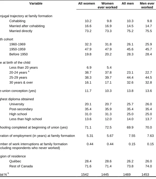
Table 1 - Distribution of respondents and mean values for selected characteristics included in the analysis

Variable All women Women

ever worked

All men Men ever worked

Conjugal trajectory at family formation

Cohabiting 10.2 9.8 10.3 9.8

Married after cohabiting 16.6 16.9 14.5 14.7

Married directly 73.2 73.3 75.2 75.5

Birth cohort

1960-1969 32.3 31.8 26.1 25.9

1950-1959 47.9 47.9 45.6 45.7

Before 1950 19.8 20.2 28.3 28.4

Age at birth of the child

Less than 20 years 6.9 5.4

20-24 years a 38.7 37.8 23.1 22.7

25-29 years 38.3 39.7 44.4 44.5

30 years & over 16.1 17.1 32.6 32.8

Pre-union conception (yes) 11.7 10.3 13.8 13.6

Highest diploma obtained

University 20.1 20.7 25.7 26.0

Post-secondary 35.4 35.9 35.4 35.4

High school 31.0 31.3 25.0 25.0

Less than high school 13.6 12.0 14.0 13.7

Schooling completed at beginning of union (yes) 71.1 72.5 69.9 70.0

Duration of employment (in years) at family formation 5.31 5.67 7.55 7.63

Number of work interruptions at family formation (excluding respondents who never worked)

0.44 0.44 0.15 0.15

Region of residence

Québec 28.4 28.6 26.2 26.0

Rest of Canada 71.6 71.4 73.8 74.0

Total N b 1542 1445 1469 1453

Source: Statistics Canada, 1995 General Social Survey (cycle 10) on Family. a. Before 25 years old for men.

(22)

Table 2 – Effects of selected characteristics on the risk of family disruption, Proportional hazards estimates (exp β) a

Variable (all women) b Model 1 Model 2

Conjugal trajectory

Cohabiting 3.61*** 3.58***

Married after cohabiting 1.54** 1.53**

(Married directly) 1 1

Less than 20 years 1.49+ 1.38

20-24 years 1.00 0.98

(25-29 years) 1 1

30 years & over 0.67+ 0.66+

Pre-union conception (no) 1 1

Yes 1.25 1.28

Birth cohort

1960-69 1.51 0.37

1950-59 1.09 0.64

(Before 1950) 1 1

(University) 1 1

Post-secondary 1.35+ 0.74

High school 1.32 0.71

Less than high school 1.73* 0.91

Birth cohort X Highest diploma obtained

1960-69 Post-secondary 1.51*

Secondary 1.59*

Less than high school 1.66*

Secondary 0.97+

Less than high school 1.47+

Schooling completed at beginning of union (yes) 1 1

No 1.73*** 1.70***

Period at entering work on a regular basis

(Never) 1 1

Before 1970 0.94 1.01

1970-79 0.59 0.62

1980-89 1.07 1.10

1990-95 1.12 1.23

Duration of employment (in years) 0.99* 0.98**

Region of residence (Rest of Canada) 1 1

Québec 1.17 1.18

Source: Statistics Canada, 1995 General Social Survey (cycle 10) on Family. a. The analysis is based on 1542 female respondents (weighted sample).

***p<.001; **p<01; *p<.05; +p<.10.

(23)

Variable (women ever worked) b Model 1 Model 2

Cohabiting 3.55*** 3.58***

Less than 20 years 1.08 0.99

20-24 years 0.94 0.91

(25-29 years) 1 1

30 years & over 0.66+ 0.64+

Yes 1.43+ 1.47+

Birth cohort

1960-69 1.48+ 0.22

1950-59 1.12 0.66

(Before 1950) 1 1

(University) 1 1

Post-secondary 1.31 0.82

Less than high school 1.85* 1.01

Secondary 1.63*

1950-59 Post-secondary 1.00

Secondary 1.05+

No 1.61*** 1.59***

Employed during family epidode (no) 1 1

Yes 5.43*** 5.09***

Duration of employment (in years) 1.04** 1.04**

Number of work interruptions 1.09 1.07

Québec 1.20 1.20

Source: Statistics Canada, 1995 General Social Survey (cycle 10) on Family. a. The analysis is based on 1445 female respondents (weighted sample).

***p<.001; **p<.01; *p<.05; +p<.10.

(24)

Table 4 – Comparing relativeª risks of family disruption (coefficients derived from model 2 table 2 and model 2 table 3)

Changes through time for each level of education :

Before 1950 1950-1959 1960-1969

ALL WOMEN

University 1 0.64 0.37

Post-secondary 1 1.42 2.02*

Secondary 1 1.36 2.23

Less than secondary 1 1.61 1.83

WOMEN EVER WORKED

Post-Secondary 1 1.21 2.03*

Secondary 1 1.48 2.30*

Changes between levels of education for each birth cohort :

UNIV. P.-SEC. SEC. <SEC.

ALL WOMEN

Before 1950 1 0.75 0.71 0.91

1950-1959 1 1.65* 1.51 2.30*

1960-1969 1 4.07* 4.29* 4.49*

WOMEN EVER WORKED

Before 1950 1 0.82 0.71 1.01

1950-1959 1 1.52 1.60 2.59*

1960-1969 1 6.94* 7.49* 7.06*

Source : Statistics Canada, 1995 General Social Survey (cycle 10) on Family.

a. Relative risks for each group are obtained by multiplying the appropriate parameter estimates of table 2 and 3. The confidence interval of these coefficients is calculated by combining the variances and covariances of the estimates that define each coefficient. An asterisk (*) indicates that a coefficient differs significantly from the reference group at the 0.05 level.

(25)

Variable (all men) b Model 1 Model 2

Cohabiting 4.76*** 4.84***

Before 25 years 1.83*** 1.90***

(25-29 years) 1 1

30 years & over 1.06 1.07

Yes 1.12 1.08

Birth cohort

1960-69 1.97+ 2.86

1950-59 1.35 1.65

(Before 1950) 1 1

(University) 1 1

Less than high school 0.83 1.14

Secondary 1.86

Less than high school 1.87

Secondary 1.24

No 0.96 0.96

Period at entering work on a regular basis

Never 0.53 0.57

Before 1970 1.93+ 2.06+

1970-79 1.37 1.43

(1980-89) 1 1

1990-95 1.88 1.88

Duration of employment (in years) 1.01 1.01

Québec 1.04 1.03

Source: Statistics Canada, 1995 General Social Survey (cycle 10) on Family. a. The analysis is based on 1469 male respondents (weighted sample).

***p<.001; **p<01; *p<.05; +p<.10.

(26)

Variable (men ever worked) b Model 1 Model 2

Cohabiting 4.98*** 5.05***

Before 25 years 1.76** 1.82**

(25-29 years) 1 1

30 years & over 1.08 1.09

Yes 1.05 1.01

Birth cohort

1960-69 1.21 1.99

1950-59 1.02 1.19

(Before 1950) 1 1

(University) 1 1

High school 0.62+ 0.60

Less than high school 0.62 0.85

Secondary 0.81

Secondary 0.75

No 0.98 0.98

Employed during family epidode (no) 1 1

Yes 14.83*** 15.95**

Duration of employment (in years) 1.09** 1.09** Number of work interruptions 1.05 1.06

Québec 1.02 1.01

Source: Statistics Canada, 1995 General Social Survey (cycle 10) on Family. a. The analysis is based on 1453 male respondents (weighted sample).

***p<.001; **p<.01; *p<.05; +p<.10.

b. The variables in italics are time-covarying covariates, whose value might change through the family episode.

(27)

Table 7 – Comparing relative risksª of family disruption (coefficients derived from model 2 table 5 and model 2 table 6)

Changes through time for each level of education :

Before 1950 1950-1959 1960-1969

ALL MEN

Post-secondary 1 1.29 1.73

MEN EVER WORKED

Post-Secondary 1 0.94 1.06

Changes between levels of education for each birth cohort :

UNIV. P.-SEC. SEC. <SEC.

ALL MEN

Before 1950 1 1.10 0.76 1.14

1950-1959 1 0.86 0.75 0.64

1960-1969 1 0.67 0.65 0.65

MEN EVER WORKED

Before 1950 1 0.90 0.60 0.85

1950-1959 1 0.70 0.63 0.51

1960-1969 1 0.48 0.41 0.37

Source : Statistics Canada, 1995 General Social Survey (cycle 10) on Family.

a. Relative risks for each group are obtained by multiplying the appropriate parameter estimates of table 5 and 6. The confidence interval of these coefficients is calculated by combining the variances and covariances of the estimates that define each coefficient. An asterisk (*) indicates that a coefficient differs significantly from the reference group at the 0.05 level.