Performance of three acoustical methods for localizing whales in the Saguenay - St. Lawrence Marine Park

Research article / Article de recherche

P

O

A

M

L

W

In

T

Sa g u e n a y

— S

. L

P

Nathalie Roy1, Yvan Simard1,2 and Jean Rouat3

'Maurice Lamontagne Institute, Fisheries and Oceans Canada, P.O. Box 1000, Mont-Joli, Québec G5H-3Z4, Canada 2Marine Sciences Institute, University of Québec at Rimouski, P.O. Box 3300, Rimouski, Québec G5L-3A1, Canada 3Department of electrical and computer engineering, University of Sherbrooke, 2500 boul. de l’Université, Sherbrooke,

Québec, J1K 2R1, Canada

a b s t r a c t

Three algorithms are explored to localize fin whale calls recorded from a large-aperture hydrophone array deployed in the Saguenay— St. Lawrence Marine Park. The methods have to cope with varying sound speed in space and time, errors in time differences of arrival (TDoA) measurements in a noisy environment, and often a limited number of hydrophones having recorded a particular event. The array was composed of 5 AURAL autonomous hydrophones with a total aperture of about 40 km, coupled with 2 hydrophones from a small-aperture cabled coastal array. The autonomous hydrophones clock drifts were estimated with a level of uncertainty from timed sources and the coastal array time reference. The calls were then localized by constant-speed hyperbolic fixing, variable-speed isodiachron Monte-Carlo simulations, and a ray-tracing propagation model. The Monte-Carlo simulations generate clouds of possible localizations from the uncertainty in hydrophone positions, TDoAs and the effective horizontal sound speeds along the different source-hydrophone paths. The ray-tracing model produces a fixed grid of TDoAs which can then be consulted to find the likeliest positions of the whales. Results from the different methods are compared and their relative advantages or limitations are discussed.

r é s u m é

Trois algorithmes sont explorés pour la localisation de vocalises de rorqual commun enregistrées par un réseau d'hydrophones à large ouverture déployé dans le Parc Marin du Saguenay-Saint-Laurent. Les méthodes doivent composer avec une vitesse du son variable dans l'espace et le temps, des erreurs dans les mesures des différences de temps d'arrivée (DTA) avec un environnement bruyant, et souvent un nombre limité d'hydrophones ayant capté un événement donné. Le réseau était composé de 5 hydrophones autonomes AURAL avec une ouverture totale d'environ 40 km, couplé avec 2 hydrophones d ’un petit réseau côtier. La dérive des horloges des hydrophones autonomes a été évaluée avec un niveau d ’incertitude à l'aide de sources aux temps connus ainsi que de la référence temporelle du réseau côtier. Les vocalises ont ensuite été localisées par la méthode à vitesse constante des hyperboles, par celle à vitesse variable des isodiachrones avec simulations de Monte-Carlo, et par un modèle de propagation de rayons. Les simulations de Monte-Carlo produisent des nuages de localisations possibles à partir des incertitudes sur les positions des hydrophones, sur les DTAs et sur les vitesses horizontales effectives du son le long des différentes trajectoires source-hydrophone. Le modèle de propagation des rayons produit une grille fixe de DTAs qui est ensuite consultée pour trouver les positions les plus probables des baleines. Les résultats des différentes méthodes sont comparés et leurs avantages ou limites relatives sont discutés.

1.

Continental shelf marine environments are challenging for acoustic localization methods because of varying complex bathymetry, 3D oceanographic processes affecting temperature and sound speed time-space structures, especially at tidal and seasonal frequencies. Localization from TDoAs on short distances also requires high time precision with special care given to clock synchronization of the array and time drifts during mid- and long-term deployments. The most used localization method, hyperbolic fixing (Spiesberger and Fristrup 1990), assumes constant speed over the 2D or 3D localization space. The source location is assumed to be a linear function of travel

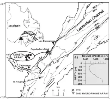
time differences, speed of sound and receiver locations. Errors in localization can be large when these assumptions are not satisfied and uncertainties in the input data are present (e.g. Spiesberger and Wahlberg 2002). These conditions generally prevail in the study area at the head of the Laurentian Channel in the St-Lawrence Estuary, where the summer sound speed profile is characterized by a well- defined channel at intermediate depths (e.g. Fig. 1a), 3D physical processes including semi-diurnal tidal upwelling and higher frequency of internal waves or fronts resulting from the interaction of tidal currents with the complex bathymetry combining with the confluence of several estuarine water masses (e.g. Saucier and Chassé 2000).

Park, w ith bathymetry, locations o f the 5 A UR A L M l autonomous hydrophones and the 6-hydrophone coastal

array, CTD station and sound speed profile. Three methods have been explored here to compare their localization performance using an array which includes autonomous hydrophones, each having its own clock, under this general context of considerable uncertainty in input data. They are the hyperbolic fixing (Spiesberger and Fristrup 1990, Spiesberger 1999, 2001), the isodiachron method with Monte-Carlo simulations (Spiesberger and Whalberg 2002, Spiesberger 2004) and the use of an acoustic propagation model (Tiemann and Porter 2004).

2. M A T ER IA L A ND M ETH O D S

Data collection

The hydrophone arrays were deployed in the study area during summer 2003 (Fig. 1). All hydrophones were HTI 96-min with a nominal receiving sensitivity (RS) in the low frequency band (< 2 kHz) of -164 dB re 1 V/^Pa. Five AURAL autonomous hydrophone systems (Multi- Electronique Inc, Rimouski, Qc, Canada) programmed to sample continuously 16-bit wave data over the 1 kHz band were deployed as oceanographic moorings. The hydrophones were placed at intermediate depths in the water column close to the summer sound channel axis. Special care was taken to minimize possible noise sources from the moorings. The outer 2 hydrophones from a 650-m aperture cabled coastal array deployed along Cap-de-Bon-Désir (Fig. 1,) completed the 7-hydrophone data base used in this study. The acquisition system for the coastal array was a 16- bit ChicoPlus Servo-16 data acquisition board (Innovative Integration, Simi Valley, CA, U.S.A.). After analysis of the recordings, this beta version of AURAL M1 was found to have a clock drift of about 18 s per day, consistent on all 5 instruments. The coastal array's PC clock had a drift of about 10 s per day, which was checked and corrected every weekday morning. The coastal and AURAL arrays were

synchronized using simultaneous recording of the same acoustic signals such as motor boats and whale vocalizations, and linear time interpolations assuming constant drift. Timing errors are inherent to such a procedure and the localization method must be robust enough to deal with such uncertainties as well as the non spatially homogenous effective sound speed.

24 20 — 2 4 ­ 2 0 - _ 24 - f I 2 0 -Iii i ^ il ià i 11 ii i i J

p

!

Figure 2. Binarized im age o f spectrogram from a fin whale series o f calls from 6 hydrophones o f the array. A typical sound speed profile from a CTD cast made in the area is shown in Fig. 1a.

Data analysis

The 80-s sample used for localization is a series of fin whale pulse calls in the 18-25 Hz frequency band (Fig. 2) recorded Sept. 24 at 4:49 local time. This sample was detected on all hydrophones except one where background noise was masking the call. The TDoAs between hydrophones is determined by spectrogram cross

Figure 3. Ray m odel grid o f 1000 points covering 20 x 50 km in the area o f study and associated with the 7 receiver

coincidence (e.g. Simard et al. 2004), after bandpass filtering to [18 25] Hz.

A constant sound speed of 1450 m s-1, corresponding to the average speed in the sound channel where the hydrophones were deployed, was used for hyperbolic analysis and as the central speed of the interval used in isodiachron Monte-Carlo applications.

The 1-km resolution grid used for the ray-tracing Bellhop model (Porter and Liu 1994) covered an area of 20 x 50 km enclosing all hydrophones (Fig. 3). The typical sound speed profile of Fig. 1a was used for the modeling. For each grid point, a set of TDoAs was calculated assuming a source at a depth of 10 m, a frequency of 500 Hz, and using 21 rays in the ±20o directions along the propagation path plane. The bathymetry profile between source and receiver was extracted from a high-resolution multibeam bathymetry dataset provided by the Canadian Hydrographic Service. The mean times of ray arrivals, weighted by ray amplitudes, provided by Bellhop for the array configuration were then used for TDoA calculations. The sound source was located at the minimum Euclidean distance between measured and modeled TDoAs (Tiemann and Porter 2004).

Isodiachrons are an extension of the hyperbolic location method but where the effective sound speed along the path between source and each receiver is allowed to vary from path to path. Receivers are combined in groups of three, which gives a total of 20 groups from 6 receivers. For each group, sound speed, receiver positions and TDoAs are treated as uniformly distributed random variables within a chosen interval that is the best educated guess of data uncertainty. Monte-Carlo simulations are then applied to produce a probability density function (pdf) of source location, called a constellation, for each group of 3 receivers. The actual source is then located within the intersection of all the constellations at the most probable

Eastings (km)

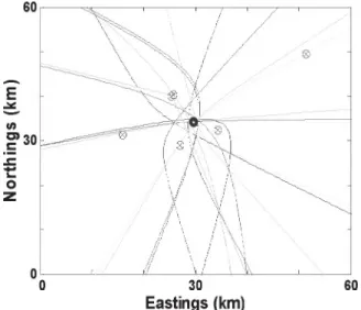
Figure 4. 2D hyperbolic localization o f the fin w hale calls. H ydrophone positions are illustrated as crossed circles.

W hale position is the bold circle.

50 IT 40 (0 S 30 o u o r 20 «

2

Figure 5. Localization o f fin w hale on the ray-tracing model grid. The receivers are illustrated by stars; the whale position is a crossed circle in the darker zone o f the figure. Background grayscale image represents difference between

measured and modeled TDoAs; smaller differences are darker. W hite patches are areas w here a source would not

be heard by all receivers.

position from the joint probability distribution function (pdf) along X and Y dimensions (i.e. 2D histogram) of all solutions.

3. R E S U L T S

Resulting hyperbolic fixing from the set of TDoAs is presented in Fig. 4. The position found for the fin whale is 48.214° N, 69.408° W, within the center of the array configuration. Estimated fixing error on this result is 1690 m, derived from the norm of the differences between

0 30 60

Eastings (km)

Figure 6. Localization process using isodiachron technique with M onte-Carlo simulations. The receivers are illustrated by crossed circles. Different constellations are

shown in shades o f gray. The estimated w hale position is represented by a diamond.

estimated and measured time along every path (Simard et al. 2004).

The same set of TDoAs was applied to the ray tracing TDoA estimation grid to produce results shown in Fig. 5. The background grayscale image represents difference between measured and modeled TDoAs; smaller differences are darker. The whale position is in the darkest area of the grid at a position of 48.220° N, 69.384° W. Grid size implies an uncertainy of at least ± 1 km.

Fig. 6 illustrates results obtained from the isodiachronic Monte-Carlo method. Each constellation was obtained from 4000 different estimates of source location from a varying set of input values for receiver location, sound speed and TDoAs. Assumed errors for these variables were ± 20 m, ± 5 m s-1 and ± 1.0 s respectively. The 1.0 s error is the minimal value needed to obtain intersection of all constellations. The region of intersection is a 600 x 800 m rectangle, the presumed position of the source being where the density is highest. The estimated whale position is 48.216° N, 69.421° W. Confidence intervals for 95% of the pdf are 580 m for x and 770 m for y.

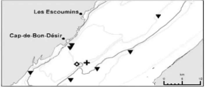
Figure 7 shows the whale positions obtained from the three methods. The isodiachron result is at 1.01 km from the hyperbolic position and at 2.24 km from the result of the ray-tracing model grid.

4.

DISCUSSION

The whale was localized in one of the 3 intensive feeding spots found at the head of the Laurentian channel (Mingelbier and Michaud 1996), where tidal upwelling along the slope concentrates krill in dense demersal patches

L e s E s c o u m i n s # ▼ C a p - d e - B o n - D é s ir# J —

-jj

*

Figure 7. Locations o f fin w hale from the three methods: diam ond for isodiachron, circle for hyperbolic result and

cross for ray-tracing m odel grid. The receivers are illustrated by triangles.

(Cotté and Simard 2005) that are exploited by fin whales from tagging experiments (e.g. Simard et al. 2002 Fig. 3b1). We observed strong whale blows (either from fin or blue whales) from the coastal array location at Cap-de-Bon-Désir on the north shore on the same morning during daylight, which were about 4 km from the localized fin whale, 6 hours later; so the localization found by the three methods is very likely given the fidelity to the feeding site over several hours.

This localization example illustrates the need for high precision in the set of variables involved in the localization problem and an accurate propagation model, which is difficult to satisfy because of technical constraints due to complex water mass structure combined with complex bathymetric characteristics. The isodiachron Monte-Carlo technique indicated that the error on TDoAs was in the order of 1 s. Even if the whale is favourably positioned at the center of the array, both the hyperbolic and ray-tracing solutions have uncertainties exceeding 1 km, given a 1-s travel time at 1450 m s-1. In both cases, an estimate of the confidence interval of the localization reflecting uncertainties in the input values would be needed (c.f. Spiesberger and Wahlberg 2002), but is not formally provided by the methods. As mentioned by Tiemann and Porter (2004), a Monte-Carlo approach could be used to evaluate uncertainties in localization by incorporating the measurement error in TDoAs. However, the uniform sound speed profile over the entire grid is an unrealistic model condition that would also require special attention in such variable environments. This would add substantial modeling efforts. Monte-Carlo simulations can also be applied to the hyperbolic method to find the optimal effective homogeneous sound-speed, which corresponds to the isodiachron particular case when the sound speed is constant. Indeed, what we found most useful in the isodiachron Monte-Carlo method is the application of pdfs to evaluate input error magnitude.

Our estimation of source location is done by finding the area of highest density on a 2D histogram of all possibilities in the overlapping constellation area. Spiesberger and Wahlberg (2002) used separate pdfs along X and Y dimensions to compute the confidence interval of the solution. We found the joint 2D pdf more practical in a context of comparing method precision and also for whale tracking purposes, where a best estimate of whale position has to be extracted. However, the 2D histogram becomes useless if very few points are present in the constellation intersection area, or when two or more equivalent peaks are found in the distribution. Then the computation of the center of gravity by principal component analysis might be more adapted to estimate the source localization.

Another difficulty is estimating confidence limits for the source localization. Spiesberger et al. (2002) proposed to use the x and y sizes of the constellations with the smallest confidence limits, defined as two standard deviations. We found this approach misleading when constellations are spread out in long elliptic shapes, and distributions can stretch out to 100 km or more. Our approach uses the pdf of the localizations in the constellation intersecting area. However, in both cases, the limitation of this Monte-Carlo method is the strong dependence of output confidence interval on input error bounds. They should ideally be independent.

In our test, the ray-tracing model grid's precision is limited by mesh size. Building the grid is demanding in computation time, although some degree of interpolation can be applied to reduce the number of grid points to compute. Computation time can be reduced by inverting the

source-receivers in computing the TDoAs along equally spaced directions for each hydrophone and then interpolating on the grid from the 7 propagation times (M.B. Porter pers. comm.). However, the grid has to be regenerated when a new configuration of receivers is used. Another drawback is that a position is always found on the grid even if the source is outside the domain or if measurement errors are high, which requires position validation by other means. To be fair, the grid method should be tested with measured data with a known source; it might actually outperform other methods in cases where input data have relatively small errors and where sound speed and ray trajectories are not uniform. In our case study, calls detected on more than three hydrophones were rare, due to the large aperture of the array and low number of hydrophones combined with high shipping noise (e.g. Simard et al 2006). Testing the localization from a low- frequency source would be suitable, notably for evaluating the effective sound speed and for synchronizing clocks, but such large-size and high-power sources are specialized equipments that are not easily available and deployable besides posing ethical problems because of their potential negative impact on fauna.

For future work perspective, the clock synchronization problems encountered in this initial deployment of the array in 2003 were clearly the main source of localization error. Then, at an order of magnitude lower, come the sound speed variation and the precision and accuracy of TDoA estimates. Increasing the number of hydrophones to form a denser array may improve probability of detection and reduce the localization error. Then regular sound speed profile measurements over the area could further improve the localization. Acquiring frequently updated profiles would need the regular use of a ship equipped with a CTD or sound speed profiler. Alternatively, sound speed profiles could eventually be estimated from the recorded acoustic data on the array by passive acoustic tomography techniques using the transiting merchant ships as sources of opportunity to monitor the environment in a non-invasive way (C. Gervaise, Ensieta, Brest, France, personal communication).

5.

ACKNOWLEDGEMENTS

This work was supported by the Fisheries and Oceans Canada (DFO) Chair in applied marine acoustics at ISMER- UQAR, DFO Maurice Lamontagne Institute species at risk program and FQRNT Quebec research fund. We thank the crews of the M/V Coriolis II, NGCC Isle Rouge and all the technicians, students and assistants involved in preparing the material, its deployment at sea and the data acquisition. We also thank Parks Canada Saguenay-St. Lawrence Marine Park for their steady collaboration. The computer program for applying the isodiachronic technique was developed at Sherbrooke University as part of a Master thesis. We would like to thank students Diya Seebaruth and Hansa Devi Gukhool for their invaluable support.

6.

REFERENCES

Cotté, C., and Simard, Y. 2005. The formation o f rich krill patches under tidal forcing at whale feeding ground hot spots in the St. Lawrence Estuary. Mar. Ecol. Progr. Ser. 288: 199-210. Mingelbier, M., and Michaud, M. 1996. Étude des activités

d ’observation en mer des cétacés de l’estuaire maritime du Saint-Laurent: compte rendu de l’échantillonnage de 1995 et synthèse des données prélevées de 1984 à 1995. Final report to Parks Canada, Canadian Heritage Department, Ottawa. GREMM, 108 de la Cale Sèche, Tadoussac, QC G0T 2A0. Porter, M.B., and Liu, Y.C. 1994. Finite-Element Ray Tracing.

Proceedings o f the International Conference on Theoretical and Computational Acoustics, Eds. D. Lee and M. H. Schultz (World Scientific, Singapore 1994): 947-956.

Saucier, F.J., and Chassé, J. 2000. Tidal circulation and buoyancy effects in the St. Lawrence estuary. Atmosphere-Ocean 38: 505-556.

Simard, Y, Bahoura, M. and Roy, N., 2004. Acoustic detection and localization o f whales in Bay of Fundy and St. Lawrence estuary critical habitats. Canadian Acoustics 32 (2):107-116. Simard, Y., Lavoie, D. and Saucier, F.J. 2002. Channel head

dynamics: Capelin (Mallotus villosus) aggregation in the tidally-driven upwelling system o f the Saguenay-St. Lawrence Marine Park's whale feeding ground. Can. J. Fish. Aquat. Sci. 59: 197-210.

Simard, Y., Roy, N. and Gervaise, C. 2006. Shipping noise and whales: World tallest ocean liner vs largest animal on earth. OCEANS’06 MTS/IEEE - Boston, IEEE Cat. No. 06CH37757C Piscataway, NJ, USA.

Spiesberger, J.L. 1999. Locating animals from their sounds and tomography of the atmosphere: Experimental demonstration. J. Acoust. Soc. Am. 106: 837-846.

Spiesberger, J.L. 2001. Hyperbolic location errors due to unsufficient numbers o f receivers. J. Acoust. Soc. Am. 109: 3076-3079.

Spiesberger, J.L. 2004. Geometry o f locating sounds from differences in travel time: Isodiachrons. J. Acoust. Soc. Am. 112: 3046-3052.

Spiesberger, J.L. and Fristrup, K.M., 1990. Passive localization of calling animals and sensing o f their acoustic environment using acoustic tomography. Am. Nat. 135: 107-153.

Spiesberger, J.L. and Wahlberg, M. 2002. Probability density functions for hyperbolic and isodiachronic locations. J. Acoust. Soc. Am. 112: 3046-3052.

Tiemann, C.O., and Porter, M.B. 2004. Localization of marine mammals near Hawaii using an acousic propagation model. J. Acoust. Soc. Am. 115: 2834-2843.