This is an author-deposited version published in: http://oatao.univ-toulouse.fr/ Eprints ID: 3714
To cite this document :KANG, GuoDong, PÉRENNOU, Tanguy, DIAZ, Michel, ZORZI, Francesco, ZANELLA, Andrea. Group Behavior Impact on an Opportunistic Localization Scheme. In : Future Network and Mobile Summit 2010, Florence, 16-18
June 2010
Any correspondence concerning this service should be sent to the repository administrator: [email protected]
Future Network and MobileSummit 2010 Conference Proceedings Paul Cunningham and Miriam Cunningham (Eds)
IIMC International Information Management Corporation, 2010 ISBN: 978-1-905824-16-8
Group Behavior Impact on an
Opportunistic Localization Scheme
GuoDong KANG1,3,4, Tanguy PERENNOU2,3, Michel DIAZ2,3, Francesco ZORZI5,
Andrea ZANELLA5
1T´eSA ; 16 Port Saint-Etienne, F-31000 Toulouse, France 2CNRS ; LAAS ; 7 avenue du colonel Roche, F-31077 Toulouse, France 3Universit´e de Toulouse ; UPS, INSA, INP, ISAE ; LAAS ; F-31077 Toulouse, France
4Northwestern Polytechnical University, Xian, China
5Dipartimento di Ingegneria dell’Informazione, Universit degli Studi di Padova, Italy
E-mail: {gkang,perennou}@isae.fr, [email protected], {zorzifra,zanella}@dei.unipd.it
Abstract: In this paper we tackled the localization problem from an opportunis-tic perspective, according to which a node can infer its own spatial position by ex-changing data with passing by nodes, called peers. We consider an opportunistic localization algorithm based on the linear matrix inequality (LMI) method coupled with a weighted barycenter algorithm. This scheme has been previously analyzed in scenarios with random deployment of peers, proving its effectiveness. In this paper, we extend the analysis by considering more realistic mobility models for peer nodes. More specifically, we consider two mobility models, namely the Group Random Way-point Mobility Model and the Group Random Pedestrian Mobility Model, which is an improvement of the first one. Hence, we analyze by simulation the opportunistic local-ization algorithm for both the models, in order to gain insights on the impact of nodes mobility pattern onto the localization performance. The simulation results show that the mobility model has non-negligible effect on the final localization error, though the performance of the opportunistic localization scheme remains acceptable in all the considered scenarios.
Keywords: Localization; Opportunistic network; Mobility models.
1
Introduction
The demand for mobile localization services is continuously growing as wireless network becomes more and more popular. GPS-like solutions cannot prove effective in all the cases, either because of technological or economics limits. Therefore, alternative solu-tions to provide localization services with different levels of accuracy to mobile users have been investigated. Very accurate solutions with positioning errors less than one meter are obtained by using complex triangulation algorithms coupled with sophisti-cated ranging mechanisms provided, e.g., by UWB infrastructure equipments or dense and regular WiFi access points deployment. Most of such solutions, however, are expen-sive, because they require either specific technologies/equipments or an over-provisioned infrastructure.
In this paper we tackle the problem from a different perspective: rather than search-ing for yet another signalprocesssearch-ing technique or system architecture explicitly designed to provide localization services, we propose to spill out this service from the opportunis-tic interactions that may occur among heterogeneous wireless nodes. In such a context, our previous work [1, 2] has shown that a node, named user, can infer its own posi-tion with sufficiently good accuracy simply by using posiposi-tion estimaposi-tions received from
passing by nodes, named peers. We believe that the cooperative and opportunistic ex-change of positioning information by peers is a sustainable approach. In this paper, we use a weighted opportunistic localization algorithm in which a method based on linear matrix inequalities (LMI) [10] is coupled with a weighted barycenter computation that takes into account the number of peers from which the user has received data.
In our previous study [1, 2], peers were considered as individual elements, each following a statistically independent path. Under this assumption, the proposed op-portunistic algorithm attained good localization accuracies for the user node after a rather limited number of opportunistic meetings with peers. However, in many prac-tical scenarios, peers tend to move in groups. Unfortunately, social behavior modeling is still a controversial issue and, although a few models have been published [3], there is no general consensus on any of them. In this study we investigate the impact of the peers mobility model on the performance of the opportunistic localization scheme. To this end, we propose a new mobility model, named Group Random Pedestrian Mobil-ity Model, which improves the preexisting Group Random Waypoint MobilMobil-ity Model by adding the pedestrian behavior. Then, we compare the opportunistic localization performance when considering different mobility models, ranging from the Random Waypoint model where nodes move randomly and independently one another, to the Group Random Pedestrian Model where peers trajectory are strongly correlated. We will show the localization performance generally decreases when peers move in groups, though the opportunistic approach still yields largely acceptable results.
The paper is organized as follows: Section 2 introduces the opportunistic localiza-tion schemes. Seclocaliza-tion 3 describes the group mobility models proposed in this paper. Section 4 describes the simulation setup and compares the localization accuracy ob-tained with different mobility models. Section 5 surveys related work. Conclusion and future work are given in Section 6.
2
A Weighted Barycenter Positioning Scheme
2.1 Background
The envisioned scenario entails an indoor environment, where a user node that does not have any a-priori knowledge of its own position can opportunistically exchange data with mobile peers that are within radio range. Peer nodes are supposed to be equipped with some self-localization hardware, e.g., MEMS-based Inertial Navigation System, indoors GPS or Cricket. Hence, the opportunistic interactions among nodes may be exploited so that peers provide their positioning estimates to the user node.
The position estimation scheme presented in this paper is based on the processing of several consecutive positioning information the user receives from passing-by peers. During this process, the user is assumed to stand in the same position for a certain amount of time. One aim of this paper is to determine the time the user node needs to stop to have an accurate estimation. Peer nodes, instead, are supposed to move in the area, broadcasting from time to time their current position.
2.2 Communication Model
We assume that radio communication can occur only when the received signal strength (RSS) is above a certain threshold TR, which corresponds to a nominal communication
the user-peer distance is assumed to be smaller than R and the position information of this peer is accepted. Otherwise, the position information of the peer is ignored. The use of the RSS threshold in localization scheme is much more robust and simpler than RSS-based triangulation methods which require very precise RSS-distance estimation. Additionally, we neglect potential interference problems or channel capacity issues, which will be addressed in future work.
2.3 Mathematical Model
Throughout the remainder of this paper we will denote the position of the user as Pu = (xu, yu), the position of moving node i as Pi = (xi, yi). Upon receiving and
accepting M positioning estimations from peers, the user assume that its own position lays within the intersection of M circles with radius R, centered on the Peers’ positions. This geometry relation can be expressed in mathematical form as the following set of constraints:
∀i ∈ 1 . . . M kPu− Pik ≤ R. (1)
Equation (1) can be reformulated as the following Linear Matrix Inequality (LMI):
∀i ∈ 1 . . . M R 0 xu − xi 0 R yu − yi xu− xi yu− yi R ≥ 0. (2)
The solution of this LMI problem will be regarded as the initial location estimation of the user node, which is named LMI-only location estimation and denoted by Pu,lmi.
2.4 Weighted Localization Scheme
After a period of time, the static user can collect a set of successive Pu,lmi LMI-only
estimations. The precision of LMI-only localization generally increases with the num-ber of inequalities, so we weight each estimate proportionally to the numnum-ber of nodes involved in the estimation process. The weighted opportunistic position estimation is composed by the following two steps:
1. At every second t, the User collects position information from each peer node that is within its radio range. Then the user computes its LMI-only location estimation Pu,lmi(t) according to Equation (2).
2. At the same time, the user performs a weighted barycenter computation using the LMI-only location estimations computed up to that time, obtaining the LMI+WB (Weighted Barycenter) location estimation as:
Pu,lmi +wb(t) = Pt k=1wk· Pu,lmi(k) Pt k=1wk . (3)
where wk is a weighting coefficient which is proportional to the number of Peers
3
Simulation Setup
This paper is going to show that even using group mobility models, our localization scheme can give accurate results. In contrast with individual mobility models, group mobility models are more realistic because to some extent they consider the social character of the network.
3.1 Simulation Introduction
Our simulations are executed in the Matlab 2008b environment. Matlab provides the LMI Lab toolbox to solve LMI problems. Simulations scenario is located in an area of 100 × 100 square meters. The user node is assumed to be in the center of the simulation area. We consider 100 peer nodes that randomly move in the area according to one of the mobility patterns described later on. Moving nodes are kept within the simulation area using reflection on the borders. Nodes radio range is fixed to 10 meters.
3.2 Mobility Models
In this section we present two group mobility models, namely Group Random Waypoint (GRWP) and Group Random Pedestrian (GRP). These models are based on the exist-ing individual mobility models Random Waypoint (RWP) [4] and Random Pedestrian (RP) [1].
3.2.1 Group Mobility Models
Network Model Normally, there is some kind of social or biological relations among nodes carried by people. To describe this kind of mutual relation, we adopt the clas-sical method of weighted graphs [5], which are used to represent social network. The strength of mutual relation between any node pair is represented using a value in the range [0, 1]. As a consequence, the internal relations of a N -node network can be described as a N × N relation matrix. In our analysis, we choose a simple geometric random graph as network model although it is not the most realistic graph. The social relation exists between two nodes iff they are in radio range of each other (i.e. if their Euclidean distance is less than the radio range). The diagonal of the relation matrix is conventionally set to zero. In [6] it is shown that in two or three-dimensional area using Euclidean norm can supply surprisingly accurate reproductions of many features of real biological networks.
Group Detection Group or community structure is one of the common characters in many real networks. However, finding group structures within an arbitrary network is known to be a difficult task. A lot of work has been done on that. Currently, there are several methods that can achieve that goal, such as Minimum-cut method, Hierarchical clustering, Girvan-Newman algorithm, etc. Here we adopt one of the most widely used group detection method, namely modularity maximization that detects the group structure of high modularity value by exhaustively searching over all possible divisions [7]. In real networks, the modularity value is usually in the range [0.3, 0.7]; 1 means a very strong group structure and 0 means random behavior.
Then, nodes are initially divided in groups and, successively, they start moving in the simulation area. They will follow the group constraint coupled with the individual movement pattern as referred above.
Group Random Waypoint Mobility Model (GRWP) This model is an improvement on the classical Random Waypoint model and is inspired by the Community Based mobility model [3]. The simulation area is divided into small squares with edge size equal to the radio range of the nodes (100 squares of 10 meters size in our case). Before moving, each group chooses one small square as group destination. Then, each node in the group individually chooses one position in that small square as its own destination. Hence, each node moves towards its goal with a certain speed. Here, we choose a normal probability distribution for nodes’ speed, as for the Random Pedestrian Model, instead of using the uniform speed distribution considered in the classical RWP model. Because the speed and the destination position are different for each node in a group, they will not reach their target position at the same time. The first node of a group that reaches its target within the small square will stop for a period of time sufficient for all the other nodes of its group to arrive. When all the members of the group have reached their destination, the process is repeated anew.
Group Random Pedestrian Mobility Model (GRP) This model is set up based on our individual Random Pedestrian Model. After groups setup, each node is characterized by a Relation Factor (RF) as follows [3]:
RFi = 1 n X 1≤j≤N j6=i ai,j (4)
where ai,j is the element of the relation matrix; N is the total number of the nodes
in the network; and n is total number of nodes in the network characterized by ai,j > 0.
In each group, the node which has the greatest RF will be assigned to be the head node of the group and the remaining nodes in the group will be regarded as slave nodes that will follow the head node. In this mobility model, the head node (hn) in group g follows a Random Pedestrian Model and chooses its next direction at time t as a function of its previous direction, while the slave nodes (sn) follow the head node and choose their next direction as a function of hn direction, using normal distributions:
θhng(t) ∼ N (θhng(t − 1), π/6), (5)
θsng(t) ∼ N (θhng(t), π/12). (6)
Head and slave nodes choose their next speed from a normal distribution N (1.2, 0.2).
4
Simulation Results
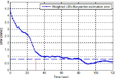
We assume the user can wait at the same position for a period of time long enough to obtain good location estimation, i.e. the final error can meet his requirement. Fig. 1 shows an example of the localization error evolution over time, assuming peers move-mements follow the RWP model. The localization error curve reaches an accuracy threshold as waiting time increases. The horizontal dashed line is the mean accuracy. It is computed as the mean of the error curve between times [30 120], where 30 s is the default warm-up time.
In Table 1, by running 50 times the simulation with different random seeds, we com-pare the effect of the waiting time on the final localization accuracy for each considered
Figure 1: A localization error curve example.
Waiting time (min) 1 2 3 4 5 RWP Mean (m) 1.06 0.73 0.58 0.49 0.44 RWP Std (m) 0.55 0.30 0.22 0.18 0.16 RP Mean (m) 1.46 1.22 1.08 0.97 0.90 RP Std (m) 0.70 0.56 0.47 0.41 0.36 GRWP Mean (m) 1.71 1.50 1.36 1.25 1.17 GRWP Std (m) 0.75 0.72 0.62 0.55 0.50 GRP Mean (m) 2.15 1.83 1.57 1.42 1.30 GRP Std (m) 1.05 0.42 0.62 0.57 0.53
Table 1: Accuracy results.
mobility model. As expected, the mean localization error decreases as the waiting time increases: 2 minutes are generally enough to achieve satisfying localization (e.g. about 1 m for RWP).
The weighted LMI+barycenter mean error increases in the following order: RWP, RP, GRWP and GRP. The good performance of RWP is due to its randomness and the known issue that with this model mobile nodes are more likely to go through the center of the area, exactly where the user is located. Therefore during the waiting time, the user can almost always find position information of peer nodes available although the number of passing through peers will be different at different time. Compared with RWP, the RPs randomness is lower. And they dont always have the opportunity to pass through the center of the simulation area therefore it may happen that no peers are in the user coverage range. This is why the accuracy obtained from RP is slightly lower than RWP. This problem is magnified in the group models GRWP and GRP. When nodes move in group, the user experiences different situations: sometimes a lot of nodes communicate with it, sometimes no one is in the coverage range. The time interval in which the user cannot find even one peer will be even longer than these two individual mobility models since these nodes begin to move in group. This will decrease the accuracy further.
5
Related Work
In [8] Doherty et al. pioneered the semi-definite programming (SDP) method in lo-calization problem. The lolo-calization problem is tried to be considered as a bounding problem containing several convex geometric constrains with the mathematical repre-sentation of linear matrix inequalities (LMI). However, in this paper no mobility is applied. Nodes are assumed to be static. The Centroid localization method [9] is de-veloped to estimate the users location by computing the barycenter of all the positions received from those fixed beacon nodes. By placing four beacon nodes at four corners of a square testing area, an average localization accuracy of with the standard deviation of can be obtained. However, in practice, a uniform placement is not always feasible. To find the optimum deployment of those beacon nodes for a given application may consume a lot of labor. The APIT method [10] is an iterative algorithm based on the use of triangle intersections, the triangle vertices being static beacon nodes. It can be iterated until a given precision is reached, altough in some cases the so-called APIT test may fail. Other research works jointly solve the time synchronization and localization problems. For instance, Enlightness [11] relies on the availability of beacon nodes (at least 5% of the nodes) providing absolute time and space information, like the GPS in outdoor environments. Enlightness combines recursive positioning estimation [12] with a clock offset estimation scheme based on the measure of beacon packet delays and timestamps.
6
Conclusion and Future Work
In this paper we have demonstrated the impact of the mobility model used on the evaluation of the accuracy of our weighted LMI+barycenter localization scheme. The obtained accuracy varies from below 1 meter to below 3.5 meters using the same setup with different mobility models. Taking into account groups decreases the performance. However, the obtained accuracy is still acceptable in many scenarios.
It should be noted that in [13] the real traces from Dartmouth College and UCSD show a power law distribution with respect to inter-contact time. From this point of view, it may imply that the two group models in this paper are still not the most realistic ones. The reason may lie in the assumption that nodes are not allowed to move among different groups. This will be improved in our future work. However, the models used here take into account many features that the individual models do not consider, making results more accurate.
In the future developments, we will consolidate this work by relaxing a number of assumptions. We will investigate the relationship between the monitored RSS and a maximum distance for WiFi radios. We will introduce a more realistic communication channel taking into account noise and interferences, and drifting self-estimations of peer positions with periodic reset, and exploit new public mobility traces.
Acknowledgements
This work was partly supported by the European Commission in the framework of the FP7 Network of Excellence in Wireless COMmunications NEWCOM++ (contract n. 216715) and by the French ANR FIL project. The authors would like to thank E. Conchon, A. Bardella and F. Fabbri for valuable discussions on this topic.
References
[1] G. Kang, T. P´erennou, and M. Diaz, “Barycentric Location Estimation for Indoors Localization in Opportunistic Wireless Networks,” in Proc. of FGCN 2008, (Sanya, China), December 2008.
[2] F. Zorzi, G. Kang, T. P´erennou, and A. Zanella, “Opportunistic localization scheme based on linear matrix inequality,” in Proc. of WISP 2009, (Budapest, Hun-gary), August 2009.
[3] M. Musolesi and C. Mascolo, “Designing mobility models based on social network theory,” ACM SIGMOBILE Mobile Computing and Communication Review, vol. 11, July 2007.
[4] J. Broch, D. Maltz, D. Johnson, Y. Hu, and J. Jetcheva, “Multi-hop Wireless Ad Hoc Network Routing Protocols,” in Proc. of Mobicom 1998, (Dallas, TX, USA), October 1998.
[5] D. J. Watts and S. H. Strogatz, “Collective dynamics of ’small-world’ networks,” Nature, vol. 393, pp. 440–442, June 1998.
[6] N. Prˇzulj, D. G. Corneil, , and I. Jurisica, “Modeling Interactome: Scale-Free or Geometric?,” Bioinformatics, vol. 20, no. 18, pp. 3508–3515, 2004.
[7] M. Newman and M. Girvan, “Finding and Evaluating Community Structure in Networks,” Physical Review E, vol. 69, no. 2, 2003.
[8] L. Doherty, L. E. Ghaoui, and K. S. J. Pister, “Convex Position Estimation in Wireless Sensor Networks,” in Proc. of IEEE Infocom, (Anchorage, AK, USA), April 2001.
[9] N. Bulusu, J. Heidemann, and D. Estrin, “GPS-less Low Cost Outdoor Localization for Very Small Devices,” IEEE Personal Communications Magazine, vol. 7, no. 5, pp. 28–34, 2000.
[10] T. He, C. Huang, B. M. Blum, J. A. Stankovic, and T. Abdelzaher, “Range-free localization schemes for large scale sensor networks,” in Proc. of the MobiCom 2003, (San Diego, CA, USA), September 2003.
[11] A. Boukerche, H. A. B. F. de Oliveira, E. F. Nakamura, and A. A. F. Loureiro, “Enlightness: An enhanced and lightweight algorithm for time-space localization in Wireless Sensor Networks,” in Proc. of ISCC 2008, (Marrakech, Morocco), July 2008.
[12] J. Albowicz, A. Chen, and L. Zhang, “Recursive Position Estimation in Sensor Networks,” in Proc. of ICNP 2001, (Riverside, CA, USA), November 2001.
[13] A. Chaintreau, P. Hui, J. Crowcroft, C. Diot, R. Gass, and J. Scott, “Pocket Switched Networks: Real-world mobility and its consequences for opportunistic forwarding,” Computer Lab. Technical Report UCAM-CL-TR-617, University of Cambridge, February 2005.