Taylor bubble moving in a flowing liquid in vertical channel: transition from symmetric to asymmetric shape

This is an author-deposited version published in: http://oatao.univ-toulouse.fr/ Eprints ID: 4884

To link to this article: DOI:10.1017/jfm.2011.159 URL : http://dx.doi.org/10.1017/jfm.2011.159

To cite this version: Figueroa, B. and Fabre, J. Taylor bubble moving in a flowing

liquid in vertical channel: transition from symmetric to asymmetric shape. Journal

of Fluid Mechanics, 679 . pp. 432-454.

O

pen

A

rchive

T

oulouse

A

rchive

O

uverte (

OATAO

)

OATAO is an open access repository that collects the work of Toulouse researchers and makes it freely available over the web where possible.

Any correspondence concerning this service should be sent to the repository administrator: staff-oatao@inp-toulouse.fr

17/03/11 1

Taylor bubble moving in a flowing liquid in vertical channel:

transition from symmetric to asymmetric shape

BERNARDO FIGUEROA-ESPINOZA1 and JEAN FABRE2 1

Instituto de Ingeniería, Universidad Nacional Autónoma de México, Calle 21 # 97A, Col. Itzimná, 97100, Mérida, México

2

Institut de Mécanique des Fluides, Institut National Polytechnique de Toulouse Allée du Prof. Camille Soula, 31400 Toulouse, France

The velocity and shape of Taylor bubbles moving in a vertical channel in a Poiseuille liquid flow were studied for the inertial regime, characterized by large Reynolds numbers. Numerical experiments were carried out for positive (upward) and negative (downward) liquid mean velocity. Previous investigations in tube have reported that for upward flow the bubble is symmetric and its velocity follows the law of Nicklin whereas for certain downward flow conditions the symmetry is broken and the bubble rises appreciably faster. To study the bubble motion and to identify the existence of a transition, a 2D numerical code that solves the Navier-Stokes equations (through a VoF implementation) was used to obtain the bubble shape and the rise velocity for different liquid mean velocity. A reference frame located at the bubble tip as well as an irregular grid were implemented to allow for long simulation times without an excessively large numerical domain. It was observed that whenever the mean liquid velocity exceeded some critical value, bubbles adopted a symmetric final shape even though their initial shape was asymmetric. Conversely, if the mean liquid velocity was smaller than that critical value, a transition to a non-symmetric shape occurred, along with a correspondingly faster velocity. It was also found that surface tension has a stabilizing effect on the transition.

17/03/11 2

1. Introduction

The motion of long, bullet shaped bubbles in the interior of tubes —also known as Dumitrescu-Taylor bubbles— is relevant for a wide variety of engineering systems in the nuclear, oil, petrochemical or aerospace industries and for some natural phenomena like volcanic eruptions. Some of the first investigations on this subject were presumably motivated by submarine related research during the Second World War. Among these studies, it is worth mentioning the pioneering works of Dumitrescu (1943) and Davies & Taylor (1950) who explained the inertial motion of a long bubble rising in still liquid with an irrotational solution of the local flow field in the vicinity of its apex. These two studies were the starting point of a long series of experimental, theoretical and numerical investigations on the motion of Taylor bubbles in vertical tube. The key observation that permitted this development is that these large bubbles move as if viscous and surface tension forces were small compared to inertial effects. In the present work we shall focus on the influence of the flowing liquid on the motion of a plane bubble in the inertial regime. Because the behaviour of such bubbles is similar to that of Taylor bubbles in tube we will recall first some of the major findings in cylindrical geometry.

Nicklin et al. (1962) were the first to present a comprehensive study of the bubble dynamic in upward flow. From their experiments they found that the bubble velocity V* is given by:

(1)

!

V* =C₀U*+V_"*, (1)

where U* _{is the mean liquid velocity and}

!

V_"* the bubble velocity in still liquid. Note that the starred quantities are made dimensionless using the radius D/2 as a length scale and

!

gD as a velocity scale, g being the gravity. The velocity in still liquid depends slightly on surface tension _{σ and kinematic viscosity ν. As such it can be expressed as a weakly}

17/03/11 3

varying function

!

V_"*(# , N ) of the dimensionless surface tension and viscosity ! "=4# / $gD2 and ! N ="/ gD3.

At small viscosity and surface tension,

!

V_"*(0,0)=_{0.35 and}

!

C₀ is about 2 (resp. 1.2) for laminar (resp. turbulent) flow. Nicklin et al. (1962) pointed out that ! V* "UM * + V_#*_{, where} ! UM *

is the axis liquid velocity far upstream. In addition to the influence of flow regime, C0 is slightly modified by surface tension. As a result it can be expressed as a function of the Reynolds number and the dimensionless surface tension:

!

C₀( Re," ) . For more details, see for example Wallis (1969) or Fabre & Liné (1992). These results were confirmed by analytical solutions (e.g. Collins et al. 1978) and by numerical solutions of either full Navier-Stokes equations (e.g. Mao & Dukler 1990) or Euler equations using boundary element (BE) method (Ha Ngoc & Fabre 2006). Note that these studies are 2D calculations for bubbles with prescribed axis-symmetric shape. Although theoretical analysis and numerical simulations have been able to predict the velocity and shape of symmetric bubbles in tube, some unsolved issues of practical relevance still remain in downward liquid flow. For some flow conditions Griffith & Wallis (1961) observed that the bubble motion is unstable and moves closer to the wall adopting an asymmetrical shape. Martin (1976) and later on Polonsky et al. (1999) found from specific experiments in downward flow that when the bubble is asymmetric it rises appreciably faster than expected from an axis-symmetric bubble facing the same liquid velocity profile.

To throw light on this issue Lu & Prosperetti (2006) performed an analytical stability analysis of the bubble shape with zero surface tension and demonstrated that there exists a downward velocity threshold of approximately

!

U_c* " #0.13 below which the bubble looses its symmetry with respect to the axis. According to them, this happens

17/03/11 4

presumably because the relative velocity between the bubble and the liquid decreases with increasing downward flow, which is also accompanied by a flattening of the bubble nose. Both conditions have a destabilizing effect on the bubble configuration.

The aim of this work is to shed some light on this transition and the effect of surface tension on the bifurcation. In this numerical study, the problem of a single Taylor bubble rising in a flowing liquid is undertaken with the aid of a numerical code called

JADIM, developed at the Institute of Fluid Mechanics of Toulouse, France. The VoF

version of this code has been used and updated by several contributors for almost fifteen years to solve a great variety of fluid dynamics problems (see Benkenida & Magnaudet 2000, Bonometti & Magnaudet 2007, Dupont & Legendre 2010, and references therein).

This document is organized as follows. In Section 2 we justify the numerical experiments carried over in this work in 2D channels and we recall the previous results obtained in this particular geometry. Next we present the code description, its implementation and the validation tests in Section 3. Then we show the numerical results obtained for various flow conditions in Sections 4 and 5. Finally a brief discussion of the results and the corresponding conclusions are posted in Section 6.

2. Numerical experiments in 2D channels

If the symmetry of a bubble in a tube is broken, the flow field becomes necessarily 3D, while an asymmetric plane bubble remains 2D. However 2D plane bubbles are not physical since it is not always possible to reproduce 2D bubbles moving in a 2D flow by means of an experiment in a rectangular channel of large enough depth-to-width aspect ratio (see Figure 6 in Collins 1965). Indeed while the flow is controlled by the channel width, the bubble would be a slave of its largest curvature radius which would be of the order of magnitude of the channel depth (see Clanet et al. 2004). It is worth noting one exception. In a Hele-Shaw cell the aspect ratio has to be as small as

17/03/11 5

possible for the flow to be irrotational. Then it is possible to mimic a 2D bubble moving in still liquid as Collins (1965) and Maneri & Zuber (1974) did.

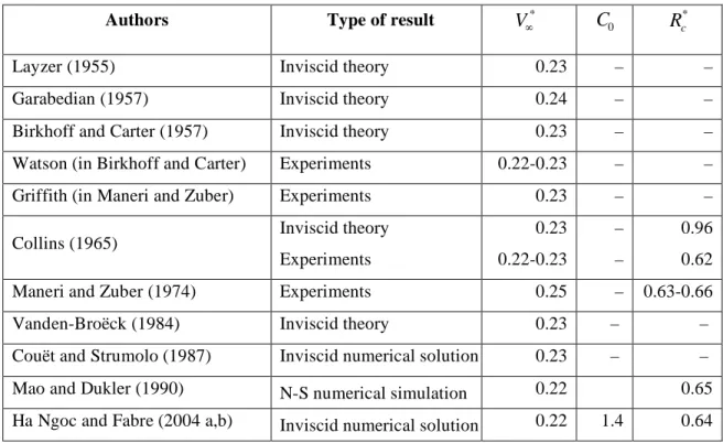
Even if 2D plane bubbles are not physical many arguments are in favour of their study. The first argument is obviously related to computational resources: the time ratio between 3D and 2D calculations is at least equal to the number (32, 64 and may be more) of azimuthal planes; it can be even much greater considering the fact that a plane bubble that looses its symmetry is likely reaching a steady asymmetric shape whereas an asymmetric bubble in tube may also rotate without reaching a steady shape. The second argument is that, as far as we are aware, numerical simulations of inertial 2D deformable Taylor bubbles mounting in downward flow, taking into account viscosity and surface tension remain hitherto unexplored. The third argument is related to the physical pertinence of 2D calculations: two-dimensional versions of real problems are usually seen as oversimplifications but whenever the difference between the real and the simplified cases remains only quantitative the 2D game deserves to be played. Last but not least we consider the 2D case as a reasonable starting point for a systematic and original investigation. Most of the results that will be discussed in the present section are grouped in Table 1.

Plane bubbles have already been considered in the past by several authors. Let us mention first the seminal work of Layzer (1955), whose motivation was rather an astrophysics problem: a first order approximation of the velocity potential around a Taylor bubble allowed for the estimation of both its velocity and the growing rate of a perturbation at the tip due to Rayleigh-Taylor instability. Using again

!

gD as the velocity scale where D is now the channel width, the theoretical rise velocity writes:

(2)

!

V_"0* =

17/03/11 6

where

!

V_"0* _{is used for}

!

V_"*(0,0). Recent investigations, like that of Kull (1983) or Clanet et

al. (2004) are based or inspired on this work.

Garabedian (1957), Birkhoff & Carter (1957) and Collins (1965) used complex variable representations of the flow field to study plane Taylor bubbles. Garabedian results showed that the solution is not unique, and suggested that the bubble shape minimizes potential energy, so the only stable configuration is the one that maximizes the bubble rise velocity. Interestingly, Birkhoff & Carter cast doubt on Garabedian maximum velocity principle, arguing that if it was true, then the symmetric bubble would be unstable because a bubble that mounts touching one of the walls is equivalent of a bubble rising in a channel of twice the width, mounting faster than the centred one.

The effect of surface tension was investigated later on: experimentally by Maneri & Zuber (1974), theoretically by Vanden-Broëck (1984), numerically by Couët & Strumolo (1987) then by Ha Ngoc & Fabre (2004 a). The numerical results showed good agreement with previous experimental and theoretical investigations †. Vanden-Broëck, motivated also by the application of these concepts on descending jets falling from vertical nozzles, used the method of Birkhoff & Carter (1957) to obtain more precise estimations of the shape and velocity. It was shown that the omission of surface tension leads to an erroneous prediction of the velocity. Correct values for zero surface tension were later obtained by solving the problem with surface tension approaching zero asymptotically. It was also shown that there exists a countable infinite number of solutions, each one corresponding to a different value of the velocity. The expected

† The numerical results of Ha Ngoc & Fabre and those of Couët & Strumolo disagree with increasing surface tension (Σ > 0.3).

17/03/11 7

physical solution was calculated as

!

V_"0* =0.226. This scenario suggests a competition between inertial and surface tension effects for the selection of the largest velocity.

Some of the aforementioned investigations give the curvature radius

!

Rc

*

at the bubble tip (Table 1). From their experiments Collins (1965) and Maneri & Zuber (1974) found 0.62 and 0.63-0.66 respectively. These results were confirmed by the numerical simulations of Mao & Dukler (1990) and Ha Ngoc & Fabre (2004 a). The theory of Collins (1965), in contrast, overestimates the curvature radius with a value of 0.96.

Authors Type of result

! V_"* ! C₀ ! R_c*

Layzer (1955) Inviscid theory 0.23 – –

Garabedian (1957) Inviscid theory 0.24 – –

Birkhoff and Carter (1957) Inviscid theory 0.23 – – Watson (in Birkhoff and Carter) Experiments 0.22-0.23 – –

Griffith (in Maneri and Zuber) Experiments 0.23 – –

Collins (1965) Inviscid theory Experiments 0.23 0.22-0.23 – – 0.96 0.62 Maneri and Zuber (1974) Experiments 0.25 – 0.63-0.66

Vanden-Broëck (1984) Inviscid theory 0.23 – –

Couët and Strumolo (1987) Inviscid numerical solution 0.23 – – Mao and Dukler (1990) _{N-S numerical simulation} 0.22 0.65 Ha Ngoc and Fabre (2004 a,b) _{Inviscid numerical solution} 0.22 1.4 0.64

Table 1. Plane Taylor bubble in vertical channels: results at small Σ.

All the previous 2D studies are related to the motion in still liquid, but what about bubbles rising in flowing liquid? As we said before a 2D experiment is probably unrealistic and it has not been carried over, contrary to numerical simulation. Ha Ngoc & Fabre (2004 b) have recently studied the motion of 2D plane bubble in upward or downward Poiseuille flow in the framework of the inviscid assumption. Their results for

!

17/03/11 8 (3) ! V*=0.23" 0.09#+

(

)

has the form of equation (1) † and that the curvature radius

!

R_c* can be expressed by a correlation that fits at best their numerical results:

(4) ! R_c* = 0.64 1

(

)

(

)

3. The numerical code

The rapid development of interface capturing methods in the last ten years allows for a choice between many different methods for multiphase flow research, like Front

tracking (see Esmaeeli & Tryggvason 1998), Volume tracking (see Harlow & Welch

1965), or VoF methods with or without interface reconstruction (see Hirt & Nichols 1981). Each method has its advantages and inherent disadvantages. For the case of choice (VoF without reconstruction), the advantages are velocity and simplicity, and the most important inconvenience is that under certain flow conditions an unphysical thickening of the numerical interface may appear (see Benkenida & Magnaudet 2000). For the case of Taylor bubbles this represents a serious drawback at the rear of the bubble, where large deformations are combined with small bubble detachment and coalescence. Nevertheless, there are some successful implementations for low Reynolds Taylor bubbles using VoF (see Benkenida 1999, Dupont & Legendre 2010). The subject has also been treated using slightly more elaborated schemes like VoF with geometric reconstruction (Taha & Cui 2006), but no successful implementations for long bubbles rising at Re=O(100) were

17/03/11 9

found in the literature. In our case the code has a treatment of the interface that cannot be considered as a reconstruction even though it improves the front stiffness. The idea is to transport both sides of the interface with the same normal velocity in reducing its thickening to a minimum (Bonometti & Magnaudet 2007). Instead of trying to simulate the rear of the bubble that has no effect at all on its velocity and shape for the inertia dominated regime, we considered infinitely long bubbles.

The code we used (referred to as JADIM) is an internal development that solves the Navier-Stokes equations for multiphase flow using the VoF method. The program is capable of solving the Navier-Stokes equations while transporting the volume fraction C, which is a scalar that represents the presence of the liquid or gaseous phase (0 for the liquid phase and 1 for the gas). In this single fluid model (Benkenida & Magnaudet 2000), the fluid properties vary abruptly across the interface, and the pressure condition due to surface tension is given by the Young-Laplace equation. The fluids are assumed to be Newtonian, incompressible and immiscible. The final scheme’s precision is of order one in time and two in space. Multiple validation tests for this code in multiphase flow situations can be found in the literature (for a more detailed discussion on the subject, see Bonometti 2003).

Studying the bubble final rise velocity usually requires long simulation times and large or periodic numerical domains. In our particular case a periodic domain would cause the perturbations at the rear of the bubble to interact with the tip, sensibly disturbing the final state. Additionally, a dense numerical mesh in the vicinity of the bubble tip is needed which combined with a large domain would result in important

† Note that if

!

V*" UM

* +

V_#* for axis-symmetric laminar or turbulent flow in tube this is far to be the case

17/03/11 10

computational cost. In order to deal with these problems, two important tasks were carried out: first a change of reference frame was implemented so as to follow the bubble tip. In the second place an irregular grid was used to comply with the required denser node length near the tip, since the bubble velocity is very sensitive to the flow conditions in its vicinity. The distance between the grid points was increased monotonically following the channel longitudinal axis with a growth rate between 0.8 and 1.2 in both directions, starting from the origin (placed at the apex of the bubble).

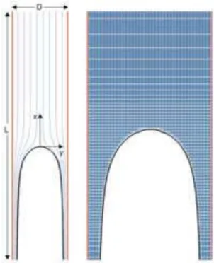
The numerical domain consisted of one section of an infinite vertical channel of width D and length L, as shown in Figure 1. The walls are vertically oriented, and the top and bottom correspond to the inlet and outlet boundary conditions respectively. Note that these conditions are often troublesome in the sense that the numerical domain truncates the physical one. At the inlet, provided the bubble obstacle is far enough, the flow may be assumed as fully developed: the parabolic velocity profile of Poiseuille flow is thus imposed. At the outlet the boundary condition has to be set to allow the liquid phase to leave the domain. However the domain truncature may result in unwanted effects like wave reflections or unbounded amplification. There exist rather elaborated schemes to deal with these problems: see for example Engquist & Majda (1977). In the present case, the outlet boundary condition is simpler. It is given by vanishing second derivatives of the normal and tangential velocities in the normal direction, and of the mixed partial derivatives of the pressure in the normal and tangential directions with respect to the outlet orientation (Magnaudet et al. 1995). The streamlines of both phases near the exit are almost parallel and reflections are observed in neither of the phases. For the liquid case, all the perturbations are swept downstream effectively due to the hydrodynamics of the films adjacent to the walls. Numerical dissipation caused by the increasing nodal

17/03/11 11

distance at the irregular grid near the outlet also helped the correct evacuation of the perturbations, so no additional artifice was needed.

Figure 1. Section of a vertical channel of length L and width D (left) and irregular nodes denser at the vicinity of the bubble tip (right). Shape and streamlines for a bubble in still liquid for Σ=0.01.

The initial conditions at the interior of the domain were as follows: at t = 0 the velocity profile along the whole channel length was parabolic

(5) ! u_"* = 3 2U * (1# y*2), v_"* =0 , (5) where ! u_"* _and !

v_"* are the components of the dimensionless velocity at the top of the domain. For the interface initial position, a section of an infinite Taylor bubble of a given initial shape was placed near the bottom, the tip being at distance l>3D from the exit. This distance was sufficient to have quasi-parallel flow in the films flowing on both sides of the bubble, at the end of the simulation. Since the final shape and velocities proved to be independent of the initial bubble shape, we implemented the simplest form that resembles a Taylor bubble: a round-tipped infinite bubble with a diameter between 0.7 D and 0.8 D. The no-slip condition was imposed on both vertical walls, y*=±1.

17/03/11 12

Preliminary tests were run for Taylor bubbles rising in stagnant liquid for 2D channels. Given that there is a thin film of liquid that flows between the channel walls and the bubble, there must be at least five to ten nodes between the bubble and the wall so as to describe correctly the flow field in this region. Consequently, the node distance in the y direction had to be readjusted after some runs. The grid length-to-width ratio was varied between 5 and 12.5, and the bubble velocity and shape became independent of this parameter for

!

L / D_{" 12.5, with a number of nodes in the x and y directions of}

! n_x" 88 and ! ny" 80 respectively.

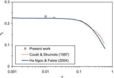
Figure 2. Velocity of a plane bubble rising in still liquid vs. dimensionless surface tension.

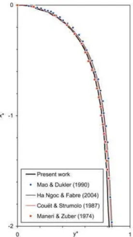
To validate the first simulations, a comparison was made with some previous results for Taylor bubbles rising in channels through stagnant liquid. Figure 2 shows a comparison of the present VoF computations against the inviscid solutions of Couët & Strumolo (1987) and Ha Ngoc & Fabre (2004 a). In the range Σ<0.025 the bubble velocity is weakly sensitive to surface tension and the present results agree with the previous ones. Finally a more detailed comparison is presented in Figure 3 in which the normalized shape of the bubble is plotted at Σ=0.01: this shape is in close agreement with those obtained from another numerical solution of the N-S equations (Mao & Dukler 1990) from experimental results (Maneri & Zuber 1974) and from numerical solutions of

17/03/11 13

inviscid flow (Couët & Strumolo 1987, Ha Ngoc & Fabre 2004 a). Even though viscosity is taken into account in our simulations, the agreement between our results and those of Couët & Strumolo or Ha Ngoc & Fabre is very good, probing the adequacy of the inviscid assumptions for the inertial regime.

Figure 3. Shape of a plane bubble rising in still liquid: comparison between 2D simulations and experiments in thin channels.

Simulations with moving liquid were also implemented for both upward and downward flow: the agreement is also satisfactory, as will be shown in the following sections.

Note that it is also possible to do simulations in an axis-symmetric geometry. These are directly comparable with experiments in tubes. Even though these simulations were also used successfully to validate the code, they are out of the scope of the present article.

17/03/11 14

Two types of numerical simulations were run: time-varying and constant U. The first type whose results are discussed in Section 4 was thought as an exploration of the bubble behaviour in a wide range of liquid velocity: U is varied slowly with time. With the second type of simulations at constant U, that will be discussed in Section 5, we intended to consolidate the previous results by ensuring that the final steady state was reached.

4. Exploratory results at time-varying U

In the present numerical experiments, the liquid velocity is varied with time. The experiment starts from a steady position either in still liquid or in upward flow. At this initial condition the bubble shape is always symmetrical. After the steadiness is reached the mean velocity U is slowly decreased down to an arbitrary negative value. Note that U is an algebraic quantity, positive (resp. negative) for upward (resp. downward) flow. Then U is increased again at the same rate. For the flow around the bubble to be quasi-steady at each time step, the time rate

!

dU / dt of the inlet flow must be as small as

possible: to comply with this condition the absolute value of the dimensionless time rate,

!

dU*/ dt* =(2g )"1dU / dt , was assigned smaller than 2.10–3 (see Table 2). As mentioned before, the flow solution depends on the dimensionless surface tension and viscosity. To remain in the inertial regime N_ν was chosen as small as possible for the viscous effects to be negligible. Three numerical experiments at Σ=0.018, 0.04 and 0.07 have been performed for capturing the surface tension effects.

Σ N dU*/dt*

0.018 5.6 10–4 0.001 0.040 8.3 10–4 0.002 0.070 8.3 10–4 0.001 Table 2. Flow conditions for time varying U*.

17/03/11 15

Two global quantities were selected for characterizing the bubble behaviour: the velocity V* _{and the asymmetry}

!

ya

*

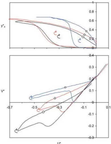
defined as the distance of the stagnation point to the axis of symmetry. They are plotted in Figure 4. It is clear from these figures, that the lines follow a different path depending on whether U* increases or decreases.

Figure 4. Exploration of the bubble velocity by varying the liquid velocity with time. Σ=0.018 (), 0.04 (), 0.07 ()

When U* decreases the path consists of three steps. In a first step, the bubble remains almost symmetric and its velocity decreases linearly: we will refer to it as the “symmetric regime” (S-regime for short). The second step is a transition regime. The symmetry breaks as the bubble tip moves closer one of the walls and its velocity increases. The third step corresponds to an “asymmetric regime” (A-regime for short). The distance of the bubble tip to the nearer wall seems to reach an asymptotic value. In the same time V* decreases almost linearly with U*.

17/03/11 16

When U* increases, the path consists of two steps corresponding to A-regime followed by S-regime. A-regime is different from that observed with decreasing U* while S-regime is the same. The trajectories in the

!

(U*,V*) plane look like hysteresis-cycles but, since these simulations represent transient phenomena, there is no warranty that the history forces remain negligible. Although these simulations are limited because of transient effect, they point out some original qualitative features.

- There exist two different regimes of motion: S- and A-regimes.

- S-regime is observed in upward liquid flow whereas, in the present numerical simulations, A-regime was observed only in downward flow.

- For a given range of downward liquid flow, either regime can be observed depending on whether U* decreases or increases.

- The bubble moves faster when it is in A-regime than in S-regime.

- The bubble motion depends on Σ in A-regime whereas it is much less sensitive to it in S-regime.

5. Results at constant U

The time-varying U experiments tell nothing about the co-existence of S- and A-regimes for a given liquid velocity. Furthermore, they remain essentially qualitative. This is why we looked for steady solutions.

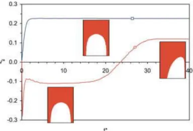
As we start each simulation from an arbitrary shape, the final solution must satisfy two conditions: (i) it must be stationary and (ii) it must not depend on the initial conditions. Starting with various initial shapes showed no significant influence on the final solution provided the transient time was large enough for the steady state to be reached. Depending on the liquid velocity, this transient time could be more or less large. Examples are given in Figure 5 where we plotted the time evolution of the bubble dimensionless velocity V* for two liquid velocities: 0 and –0.26. Note that the time

17/03/11 17

!

t*=2(g / D)1/ 2t is normalized by the time to travel over a half-diameter in agreement

with the length and velocity scales, D/2 and

!

gD, already defined. A simulation of a bubble with axis-symmetric initial shape was considered. For the first case (U*=0) it can be observed that the final velocity attains a quasi-stationary state and that the shape remains symmetric after t*≈2. Even if the simulation goes on for long time, this “stable” state persists. For the second case (U*= –0.26) a different behaviour is observed. Starting from rest there exists a strong initial transient that causes the bubble to move backwards (the velocity at t*=0 is not zero). Next, an equilibrium state appears to be quickly reached, in a time comparable to the previous case, for a bubble velocity of about V*= –0.10. The bubble shape remains axis-symmetric as indicated in the bubble picture. Later on a transition takes place and the bubble migrates to an asymmetric position along with a sensible velocity augmentation. The bubble velocity and shape stop evolving in time, notwithstanding the fact that oscillations coming from small surface waves are still present: these are later swept away to the bottom through two liquid films located between the bubble interface and the channel walls. No additional transitions are observed afterwards, even if long simulation times are attained. In this particular case the lifetime of the symmetric configuration was long: the transition usually takes place before

t*=20 and the transient time is one order of magnitude greater than for the previous case:

t*≈30. The existence of an unstable equilibrium state could be the signature of the multiplicity of solutions described by Garabedian (1957) and later on by Ha Ngoc (2003). Note that there are no artificial perturbations introduced in the flow field, with the exception of numerical noise due to truncation errors, which combined with the aforementioned oscillations are capable of triggering the transition.

17/03/11 18

Figure 5. From initial to steady state at Σ=0.018 for two liquid velocities:  U*=0,  U*=–0.26

The numerical simulations at constant-U were performed at various surface tensions: Σ=0.01, 0.018, 0.04, and 0.07. The global results are provided in Appendix for each flow condition. They include the bubble velocity, V*, the curvature radius at the bubble tip †,

!

R_c*_{, and three other important quantities that are discussed below:}

!

y_"*_,

!

y_a*

and k. The streamline passing at the stagnation point plays a special role, like for axis-symmetric bubbles: it will be referred to as the leading streamline. Two points of that streamline are important: the stagnation point whose coordinate

!

y_a* is used to quantify the bubble asymmetry and the point at infinity of coordinate

!

y_"* that allows to determine the fluid velocity at infinity. The leading streamline divides the field into two regions, each one connected with one of the liquid films flowing around the bubble. The percentage of the total liquid rate that flows through the thicker film is defined as the splitting coefficient k. For a Poiseuille velocity distribution it is connected to

! y_"* by: (6) ! k =

(

)

(

)

(

)

(

)

† The curvature radius at the bubble tip was determined as follows. A smoother shape was calculated from an exponential moving average for x ∈ [–0.1, 0]. Then it is approximated by a cubic that gives R_c*

17/03/11 19

For a symmetric bubble

!

y_a*₌

!

y_"*= 0 and k=0.5.

5.1. Influence of liquid velocity

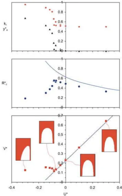
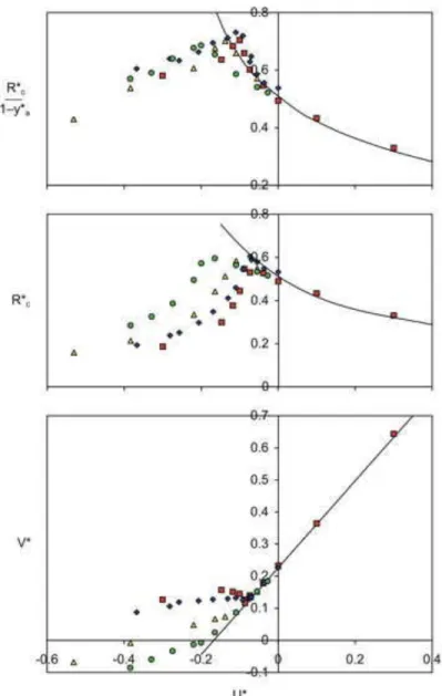
An example of results is presented in the three graphs of Figure 6 for the weakest surface tension Σ=0.01. For comparison, we added the numerical results for a symmetric bubble in an inviscid fluid obtained by Ha Ngoc & Fabre (2004 b). These graphs demonstrate clearly the existence of a transition between symmetric and asymmetric bubbles for a critical velocity

!

Uc

*

. This transition will be discussed in Sub-section 5.5.

Figure 6. Velocity (), splitting coefficient (), asymmetry ( ) and curvature radius () for Σ=0.01. Solid curves are drawn from equations (3) and (4).

17/03/11 20

When

!

U* >U_c*_{, the bubble is in S-regime as indicated by the asymmetry (}

!

y_a* =0) and the splitting coefficient (k = 0.5). Its velocity V* is a linear function of the liquid velocity U*. The agreement with the results obtained in inviscid flow is quite remarkable: they prove that the viscosity has little influence in the bubble dynamics, at least for the present dimensionless viscosity.

Concerning the curvature radius at the bubble tip, the results confirm the trend of the inviscid assumption: Rc* increases when U* decreases. Thus the bubble tip is flatter in

downward flow than in upward flow: while the curvature radius is about 0.5 in still liquid it is only equal to 0.3 for U*=0.4 and reaches a value of about 0.6 in downward flow near the critical condition. This is in qualitative agreement with equation (4) that shows that

Rc* is a decreasing function of U*. However, contrary to the bubble velocity for which the

inviscid and viscous results agree, the present curvature radii are smaller than those found by Ha Ngoc & Fabre (2004 b) in their inviscid flow simulations. The discrepancy observed here between inviscid and viscous flows could be related to the interface condition. For a viscous flow the shear stress at the gas liquid interface vanishes and the condition reads: (7) ! "s=#2 us R_c, (7)

where _{ω is the vorticity. The above condition expresses that vorticity must be created} along the curved interface to keep the velocity gradient equal to zero while the fluid rotates at the rate

!

us/ Rc. On the contrary, ω is constant on each streamline for an inviscid

plane flow and, as such, must be zero at the surface of a symmetric bubble:

(8)

!

17/03/11 21

Equations (7) and (8) are only equivalent at the stagnation point where both ωs and ωs,inv

are zero. Since

!

"=#yyy+#xxy and

!

R_c* ="xy/"xxx where ψ is the stream function, the ratio

of the curvature radii in viscous and inviscid flows at the stagnation point is given by:

(9) ! Rc * Rc, inv * = 3 5 "xxy "xxy, inv "xy, inv "xy # $ % % & ' ( ( 0 , (9) suggesting that !

R_c* <R_{c, inv}* . The present results show that this ratio is close to 0.8 so that equation (4) has to replaced by:

(10) ! R_c* = 0.51 1

(

)

(

)

It is surprising that the inviscid numerical simulations fail at predicting the curvature radius whereas they do a good job for the velocity!

When

!

U* <Uc

*

, the bubble is in A-regime. The symmetry breaking occurs in a narrow range of liquid velocity as

!

ya

*

shows. When U* _{continues to decrease,}

!

ya

*

seems to reach an asymptotic value: then the bubble tip moves close to one of the walls. Concurrently to

!

ya

*

, the splitting coefficient k increases from 0.5 to 1, indicating that most of the liquid flows through the thicker film. The curvature radius becomes smaller to that observed with symmetric bubble: the bubble is more slender so as to reduce its pressure drag against increasing downward flow. As for the bubble velocity V*, it is much greater than that it would be in S-regime and it changes little when U* decreases below the critical condition.

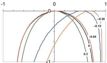
Figure 7 illustrates the effect of the liquid velocity upon the bubble shape for Σ=0.01. To fix the idea, the critical velocity

!

U_c* is equal to –0.09. When the bubble rises in still liquid or in upward flow,

U

*

" 0, the shape is perfectly symmetric. When U

*< U_c* the symmetry is broken and the bubble moves close to one of the walls with a typical

17/03/11 22

elongated tip. Nevertheless when

!

U* ="0.04 a small dissymmetry is observed: on one side the bubble keeps the shape it has in still liquid whereas on the other side it departs from this shape. Even though the bubble is not symmetric, it behaves as if it is:

!

y_a* " 0 , V* follows equation (3) and

!

R_c*, equation (10). This behaviour has been also observed in the range [

!

U_c*,0] for the other Σ-values.

Figure 7. Bubble shape for various liquid velocities at Σ=0.01 (U C *=–0.09)

5.2. Influence of surface tension

As our simulations were performed at small surface tension in the range [0.01– 0.07] we expected a marginal effect of Σ. Nevertheless even a small change of surface tension can induce drastic change on both the dynamics and the shape of the bubble. The results are indeed quite surprising as Figure 8 shows.

Whenever the bubble is symmetric we do not observe a significant influence of Σ upon either the bubble velocity or the curvature radius as equations (3) and (10) predict. However when the bubble is asymmetric, even a small difference of _{Σ may induce} significant differences. The velocity and nose curvature increase as Σ decreases. To fix the idea V* _and

!

Rc

*

experience a decrease of about 0.2 and 0.3 respectively, as Σ increases from 0.01 to 0.07. This also the case for the asymmetry but the ratio Rc

*

/(1" ya

*

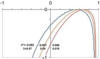
) depends little on Σ. Figure 9 illustrates the effect of surface tension for three bubbles at the same

17/03/11 23

liquid velocity. The bubble shape is mainly affected on the side of the thicker film: the smaller Σ, the more slender the bubble.

Figure 8. Influence of Σ: 0.01 (), 0.018 (), 0.04 ( ) and 0.07 (). Solid curves are drawn from equations (3) and (10) for Σ=0.01.

17/03/11 24

Figure 9. Bubble shape for various Σ at U*≈–0.37.

5.3. Flow structure and symmetry breaking

Inviscid theoretical results can be applied to Taylor bubbles moving in upward flow, since they are always symmetric. Unfortunately there are no practical results for non-symmetric bubbles. In general, the simulations proved that the flow field behaves as inviscid almost everywhere. If it were so the vorticity would be constant on each streamline and it would be also the case for the Bernoulli constant. In real flow this is the case with the exception of thin boundary layers located at the walls and very near the bubble surface. In these layers the vorticity and the Bernoulli constant depart from their values in inviscid flow. Therefore the effects of viscosity in the flow field may be quantified through the additional value that either takes on each streamline with respect to their value at infinity. Here we have chosen the additional vorticity

!

"#=#$#inv to

identify the region impacted by viscosity. For a Poiseuille flow with a velocity distribution given by equation (5),

!

"inv= f (# ) is a root of third degree polynomials in ψ

†. As such it can be calculated analytically and compared to the actual value.

† "inv 3 + U*

(

)

(

)

17/03/11 25

U*=0.3 (Re=173) U*=0 (Re=516) U*=–0.3 (Re=208)

Figure 10. Bubble shape and flow structure at Σ=0.01. Solid line: leading streamline. White arrows: velocity distribution. Additional vorticity: red area (Δω≥2), green area (1<Δω<2), blue area (Δω≤1).

Figure 10 illustrates the flow structure for bubbles that move in upward flow, still liquid and downward flow, at small surface tension (Σ=0.01). The pictures show the shape of the bubble, the additional vorticity, the leading streamline and the upstream velocity distribution. Because the _{Δω-thresholds that were chosen are somewhat arbitrary} (0, 1, 2), the layer thickness remains qualitative. As anticipated, the additional vorticity is concentrated on four viscous layers: on each wall and on either side of the stagnation point at the interface. It appears that the bubble layers are much thinner than the wall layers. Indeed, in the absence of shear stress at the interface, the only source of vorticity comes from equation (7). The analytical inviscid solutions (Dumitrescu 1943, Davies & Taylor 1950, etc.) show that the bubble dynamics is controlled by the flow in the vicinity of the stagnation point. But because the only source of additional vorticity at the bubble surface is weak the viscosity has only a marginal influence upon the bubble velocity. It

17/03/11 26

explains why the inviscid fluid assumption was so successful to predict the bubble motion.

Was the viscosity small enough to be neglected in the present experiments? According to Wallis (1969), the viscous force can be neglected whenever the dimensionless viscosity N, that can be viewed as an inverse Reynolds number, is smaller than 1/300. This condition is fulfilled in the present numerical experiments (see Table 2). For symmetric bubbles moving in still liquid and in upward flow the wall layers look the same: both start developing at a small distance from the bubble tip and begin to fill the liquid films at several unit length from it. It might be surprising that still liquid and upward flow look similar since the former is irrotational and the later rotational. Nevertheless the viscous forces remain negligible apart from the wall vicinity.

The asymmetric bubble corresponding to downward flow looks different. The boundary layer that grows at the wall wetted by the thicker film, starts at about half a diameter upstream the bubble tip whereas it starts near it at the other wall. Nonetheless if the thicker film starts developing before the other, its developing length is much greater.

The flow picture of Figure 10 suggests the mechanism of the bubble asymmetry. Even if the symmetric solution does exist theoretically, it may be unstable in some circumstance. Indeed, for the inertial regime, the driving force that tends to move the bubble upwards is balanced by momentum. One anticipates that the bubble find its path where the momentum opposed to it is the smaller. Thus one may infer from Figure 10 (b) that a bubble moving in still liquid does not see any preferential path. This is also the case of upward liquid flow as pictured in Figure 10 (a) but, because the bubble is facing less momentum at the corresponding position where the adverse liquid velocity is minimal, there is a preferential path that forces the symmetry. In contrast, when the bubble moves in downward liquid flow the bubble would normally move at the wall, as the velocity

17/03/11 27

distribution of Figure 10 (c) suggests. However surface tension comes into play to restore the symmetry (

!

U_c* <U*<0) or to prevent the bubble to stick the wall (

!

U*<U_c*). Indeed Figure 8 (c) shows that the curvature radius at the tip cannot exceed a fraction of the distance of the stagnation point to the nearer wall:

! Rc *< 3 4(1" ya * ). Because surface tension tends to make the curvature radius as large as possible, it keeps the bubble at a certain distance from the wall.

5.4. About the motion of asymmetric bubbles

The velocity of symmetric bubbles may be viewed as the additive and nearly uncoupled contributions of the fluid motion on the leading streamline and buoyancy (Nicklin et al. 1962, Collins et al. 1978). Is a similar conjecture valid for asymmetric bubbles? If this is true, the velocity of asymmetric bubbles should be given by the sum of two contributions:

- That of buoyancy is the velocity

!

V_"* that the bubble would have in still liquid with its asymmetric shape: this is of course a fictitious case since a real bubble in still liquid would be symmetrical. This contribution has to match two limiting cases. If the bubble is symmetric, i.e. when

!

ya

*=

0, equation (3) shows that

!

V_"* =0.23 regardless of the weak surface tension effects. If the bubble wets the wall, i.e. when

!

y_a*=1, it may be viewed as the half part of a symmetric bubble moving in a channel two times wider than the actual channel (Birkhoff & Carter 1957, Vanden-Broëck 1984):

!

V_"*=0.23 2 . A simple relation that matches these two limiting cases is:

!

V_"*=0.23 1+ ya

* .

- The contribution of the liquid flow can be extended from the symmetrical case. Equation (3) shows that the contribution of the liquid flow is

!

0.92 U_M* _where

!

U_M* is the velocity far upstream on the leading streamline. By extension to the asymmetric case, UM

*

17/03/11 28

With the above conjectures, the bubble velocity is given by

(11) ! Vcor * = 0.92 U*( y_"*)+0.23 1+ ya * . (11)

The estimated and actual velocities are compared in Figure 11 where symmetric and asymmetric cases are included. The agreement between numerical experiments and equation (11) is only qualitative. Moreover because

!

y_"* _and

!

y_a* have to be specified, it is not predictive. But since

!

y_"* _and

!

ya

*

are close to each other the velocity of the asymmetric bubble is about equal to

!

0.92 U*( ya

*

)+0.23 1+ ya

*

, i.e. the velocity that a symmetric bubble would have in a channel

!

(1+ ya

*

) times wider and in a Poiseuille flow specified by the maximum velocity

!

U*( ya

* ).

Figure 11. Velocity of symmetric and asymmetric bubbles, Σ=0.01 (), 0.018 (), 0.04 ( ) and 0.07 ().

Why does the bubble tip stop at a given distance from the wall? As previously mentioned there seems to be a competition between surface tension and inertia: apparently the decrease of the curvature radius in asymmetric bubbles causes a corresponding bubble velocity reduction. As a result, the bubble remains at a given position far from the wall, without touching it. It has been observed that viscosity effects are important in the falling film near the wall. This situation could create a lubrication effect, impeding the contact between the bubble and the channel wall.

17/03/11 29

5.5. Transition from symmetric to asymmetric flow

The most important issue to be discussed is certainly the transition from symmetric to asymmetric bubbles. The present results show the existence of a critical liquid velocity

!

U_c* below which the symmetry is broken. The bifurcation occurs only in downward liquid flow, i.e. for a negative value of

!

Uc

*

; it depends on surface tension and, possibly, viscosity.

To determine the transition between symmetric and asymmetric bubble several methods can be used. The first method that comes to mind is to determine directly the symmetry breaking, i.e. the liquid velocity below which

!

y_a* " 0. The other methods consist in observing the effect induced by symmetry breaking on either the dynamics, V*, or the shape,

!

Rc

*

. Therefore, the critical velocity is that below which the behaviour departs from that of symmetric bubbles predicted by equation (3) for V* and equation (10) for

!

R_c*. The methods based on induced effects almost agree with related results given in Table 3. In contrast the method based on the direct determination of asymmetry gives greater critical velocity of about –0.055, almost insensitive to surface tension. This suggests the existence of a range of liquid velocity for which slightly asymmetric bubbles behave as symmetric ones. This is a surprising result that deserves to be verified in additional experiments.

In the present study we have chosen the critical velocity obtained from induced effects (Table 3). The corresponding results plotted in Figure 12 show that when _Σ increases,

!

Uc

*

decreases almost linearly:

(12)

!

U_c* " # 2.2

(

)

However it would be risky to extrapolate the results to zero surface tension because equation (12) remains questionable at the smallest values of _{Σ. Indeed, a careful}

17/03/11 30

observation of the bubble velocity in the vicinity of the transition shows a singular behaviour for Σ=0.01 (see Figure 8).

Σ ! Uc * ! R_{c, c}* 0.010 – 0.09 0.55 0.018 – 0.08 0.59 0.040 – 0.12 0.58 0.070 – 0.19 0.60

Table 3. Critical velocity and curvature radius for various surface tensions.

Figure 12. Critical velocity  and curvature radius  vs. dimensionless surface tension.

Let us focus now on the curvature radius at the bubble tip. At critical condition it is remarkable that it is nearly equal to a maximum value of 0.6. In fact the numerical experiments that are summarized in Figure 12, show that it increases slightly with surface tension as:

(13)

!

R_c,c* " 0.22#+0.58. (13)

This is a rather strong conclusion of the present study that a symmetric bubble having a curvature radius greater than 60% of the channel half-width cannot exist.

17/03/11 31

6. Conclusions and perspectives

The case of a single Taylor bubble rising through moving liquid in a vertical channel was studied through a series of numerical experiments. Up to now, the literature mentions only few results on this particular situation, e.g. the numerical investigation of Ha Ngoc & Fabre (2004 b). Actual bubbles rising in tubes present many of the features described in the aforementioned investigation, evidencing the adequacy of the simplified inviscid assumption, and its applicability even in the 2D case. However, real bubbles present an additional feature which was not fully described by previous investigations in channel flow: if the liquid velocity decreases below some critical negative value, i.e. if the downward flow rate increases above some critical value, the flow symmetry breaks up, as shown experimentally in the past by Martin (1976) for pipe flow and the bubble rises appreciably faster than it would do if symmetry was preserved.

In this work the flow was simulated using a numerical code that solves the Navier-Stokes equations, resolving the interface position by the use of the VoF formulation. Two types of numerical experiments were carried over: when the liquid velocity varies slowly in such a way as to describe an 'aller-retour' path, the transition to the asymmetric regime is observed and the descending U branch differs from the ascending one in a hysteresis-like trajectory. However, this is not real hysteresis since the bubble always tends to a fixed point in the U-V plane when the liquid velocity variation stops, proving that the apparent hysteresis cycle results from the flow unsteadiness. These exploratory simulations also provided with the first estimates of the critical velocity. The second type of numerical experiment consisted on keeping the liquid velocity constant from the beginning, allowing the bubble to evolve freely until a quasi-steady state was reached. The transition was observed in both cases, confirming the change to a

non-17/03/11 32

symmetric regime. The reported critical velocity of the transition and bubble shape, nose position and curvature radii were all calculated using this type of scheme.

The numerical results for symmetric bubbles in upward liquid flow agree with previous theoretical and numerical results, confirming the observed 'decoupling' between the effect of transport by the liquid flow and that of bubble buoyancy. On the other hand, the non-symmetric cases provided information about the driving forces that control the different regimes: while surface tension tends to enforce symmetry, inertia forces the bubble towards the wall, where it faces a smaller amount of liquid momentum. Interestingly, the bubble never reaches the wall in these experiments. The effects of viscosity may be of importance in the liquid film that forms between the bubble and the wall. Even if the transition to a non-symmetric regime has been observed experimentally in the past, it is still one of the most original contributions of this work, since it has been closely studied through the numerical experiments. Both the velocity evolution of the bubble and the decrease of the curvature radius at the stagnation point (with increasing liquid speed) were reported: it was found that non-symmetric bubbles rise much faster than their symmetric counterparts when facing the same liquid velocity profile far upstream the bubble nose. The bubble rise velocity is very sensitive to the latter velocity profile, which in our case was parabolic. The same technique can be applied to turbulent velocity profiles, as was done by Ha Ngoc and Fabre (2004 b). It would be interesting to study those cases for two reasons: one is completeness, and the other is that for very large downward liquid velocity the bubble could actually touch the wall, presenting a second non-symmetric regime that have not yet been described.

Acknowledgements. The authors gratefully acknowledge the support of Total, S.A. We would like to thank Francis LUCK and Dominique LARREY for the interesting

17/03/11 33

experiments would have not been possible without the JADIM code, and we are grateful to Dominique LEGENDRE and Jean-Baptiste DUPONT for their clarifying comments and their help with the programming. We would also like to thanks Serge ADJOUA as well as

Annaig PEDRONO for their suggestions and coding 'tips'.

REFERENCES

BENKENIDA, A. & MAGNAUDET, J. 2000 Une méthode de simulation d’écoulements

diphasiques sans reconstruction d’interfaces, C. R. Acad. Sci. IIb 328, 25-32.

BENKENIDA, A. 1999 Développement et validation d’une méthode de simulation

d’écoulement diphasique sans reconstruction d’interface. Application à la dynamique des bulles de Taylor, Thesis, INP Toulouse, France.

BIRKHOFF, G. & CARTER, D. 1957 Rising plane bubbles, J. Math. and Mech. 6, 769-779.

BONOMETTI, T. & MAGNAUDET, J. 2007 An interface-capturing method for

incompressible two-phase flows. Validation and application to bubble dynamics, Int.

J. Multiphase Flow 33, 109-133.

BONOMETTI, T. 2003 Développement d’une méthode de simulation d’écoulements à

bulles et à gouttes, Thesis, INP Toulouse, France.

CLANET, C., HÉRAUD, P. & SEARBY, G. 2004 On the motion of bubbles in vertical tubes of arbitrary cross-sections: some complements to the Dumitrescu-Taylor problem, J.

Fluid Mech. 519, 359-376.

COLLINS, R. 1965 A simple model of the plane gas bubble in a finite liquid, J. Fluid

Mech. 22, 763-771.

COLLINS, R., de MORAES, F. F., DAVIDSON, J. F. & HARRISON, D. 1978 The motion of large bubbles rising through liquid flowing in a tube, J. Fluid Mech. 89, 497–514.

17/03/11 34

COUËT, B. & STRUMOLO, G. S. 1987 The effects of surface tension and tube inclination

on a two-dimensional rising bubble, J. Fluid Mech. 184, 1-14.

DAVIES, R. M. & TAYLOR, G. I. 1950 The mechanics of large bubbles rising through

extended liquids and through liquids in tubes, Proc. Roy. Soc. A200, 375-390.

DUMITRESCU, D. T. 1943 Strömung an einer Luftblase in senkrechten Rohr, W. Angew.

Math. Mech. 23, 139-149.

DUPONT, J. B. & LEGENDRE, D. 2010 Numerical simulation of static and sliding drop with contact angle hysteresis, J. Comp. Phys. 229, 2453-2478.

ENGQUIST, B. & MAJDA, A. 1977 Absorbing boundary conditions for the numerical

simulations of waves, Mathematics of Computation 31, 629-651.

ESMAEELI, A. & TRYGGVASON, G. 1998 Direct numerical simulations of bubbly flows.

Part I - Low Reynolds number arrays, J. Fluid Mech. 377, 313-345.

FABRE, J. & LINÉ, A. 1992 Modeling of two-phase slug flow, Annu. Rev. Fluid Mech. 24,

21-46.

GARABEDIAN, P. R 1957 On steady-state bubbles generated by Taylor instability, Proc.

Roy. Soc. A 241, 423-431.

GRIFFITH, P. & WALLIS, G. B. 1976 Two phase slug flow, J. Heat Trans. 83, 307-320. HA NGOC, H. 2003 Etude théorique et numérique du mouvement de poches de gaz en

canal et en tube, Thesis, INP Toulouse, France.

HA NGOC, H. & FABRE, J. 2004 a The velocity and shape of 2D long bubbles in inclined

channels or in vertical tubes. Part I: in a stagnant liquid, Multiphase Sciences and

Technology 16 (1-3), 175-188.

HA NGOC, H. & FABRE, J. 2004 b The velocity and shape of 2D long bubbles in inclined

channels or in vertical tubes. Part II: in a flowing liquid, Multiphase Sciences and

17/03/11 35

HA NGOC, H. & FABRE, J. 2006 A boundary element method for calculating the shape

and velocity of two-dimensional long bubble in stagnant and flowing liquid,

Engineering Analysis with Boundary Elements 30, 539-552.

HARLOW, F. H. & WELCH, J. E. 1965 Numerical calculation of time-dependent viscous

incompressible flows of fluid with free surface, Phys. Fluids 8, 2182-2189.

HIRT, C. W. & NICHOLS, B. D. 1981 Volume of fluid (VOF) methods for the dynamics of

free boundaries, J. Comp. Phys. 39, 201-225.

KULL, H. J. 1983 Bubble motion in the nonlinear Raleigh-Taylor instability, Phys. Rev.

Lett. 51, 1434-1437.

LAYZER, D. 1955 On the instability of superposed fluids in a gravitational field,

Astrophys. J. 122, 1-12.

LU, X. & PROSPERETTI, A. 2006 Axial stability of Taylor bubbles, J. Fluid Mech. 568, 173-192.

MAGNAUDET, J., RIVERO, M. & FABRE, J. 1995 Accelerated flows past a rigid sphere or a

spherical bubble. Part 1. Steady straining flow,J. Fluid Mech. 284, 97-135.

MANERI, C. & ZUBER, N. 1974 An experimental study of plane bubbles rising at

inclination, Int. J. Multiphase Flow 1, 623-645.

MAO, Z. S. & DUKLER, A. E. 1990 The motion of Taylor bubbles in vertical tubes I. A

numerical simulation for the shape and rise velocity of Taylor bubbles in stagnant and flowing liquids, J Comput. Phys. 91, 132–160.

MARTIN, C. S. 1976 Vertically downward two-phase slug flow, J. Fluids Eng. 98,

715-722.

NICKLIN, D. J., WILKES, J. O. & DAVIDSON, J. F. 1962 Two phase flow in vertical tubes,

17/03/11 36

POLONSKY, S., SHEMER, L. & BARNEA, D. 1999 The relation between the Taylor bubble

motion and the velocity field ahead of it, Int. J. Multiphase Flow 25, 957-975.

TAHA, T. & CUI, Z. F. 2006 CFD modelling of slug flow in vertical tubes. Chem. Eng.

Sci. 61, 665-675.

VANDEN-BROËCK, J. M. 1984 Rising bubbles in a two-dimensional tube with surface

tension, Phys. Fluids 27, 2604-2607.

17/03/11 37

Appendix

Numerical simulations: flow conditions (symmetry is prescribed for runs 1 to 3).

Run Σ N U* V* ! y_"* ! ya * k ! Rc * 1 0.010 1.1 10–3 -0.039 0.179 0.03 0.01 0.52 2 “ “ -0.071 0.134 0.04 0.01 0.55 3 “ “ -0.086 0.117 0.06 0.04 0.56 4 “ “ 0.300 0.643 0.00 0.00 0.50 0.33 5 “ “ 0.100 0.365 0.00 0.00 0.50 0.43 6 “ “ 0.000 0.233 0.03 0.01 0.52 0.49 7 “ “ -0.039 0.179 0.07 0.04 0.54 0.53 8 “ “ -0.074 0.140 0.17 0.12 0.60 0.53 9 “ “ -0.088 0.127 0.27 0.17 0.66 0.55 10 “ “ -0.100 0.145 0.54 0.37 0.81 0.44 11 “ “ -0.118 0.151 0.62 0.45 0.85 0.38 12 “ “ -0.147 0.157 0.70 0.53 0.89 0.30 13 “ “ -0.300 0.127 0.82 0.68 0.96 0.19 14 0.018 5.6 10–4 -0.706 0.011 0.90 0.76 0.99 0.12 15 “ “ -0.367 0.088 0.82 0.68 0.97 0.19 16 “ “ -0.282 0.106 0.79 0.63 0.95 0.24 17 “ “ -0.258 0.120 0.77 0.60 0.94 0.25 18 “ “ -0.207 0.124 0.73 0.55 0.92 0.30 19 “ “ -0.169 0.128 0.68 0.50 0.89 0.35 20 “ “ -0.131 0.131 0.59 0.42 0.84 0.41 21 “ “ -0.110 0.133 0.52 0.37 0.80 0.46 22 “ “ -0.092 0.126 0.35 0.24 0.71 0.55 23 “ “ -0.074 0.130 0.07 0.04 0.54 0.61 24 “ “ -0.070 0.135 0.12 0.09 0.57 0.59 25 “ “ -0.055 0.155 0.02 0.01 0.51 0.58 26 “ “ -0.037 0.180 0.02 0.01 0.51 0.55 27 “ “ 0.000 0.226 0.01 0.01 0.51 0.53 28 0.040 8.3 10–4 -0.531 -0.067 0.78 0.63 0.98 0.16 29 “ “ -0.384 -0.007 0.73 0.60 0.95 0.21 30 “ “ -0.219 0.049 0.59 0.45 0.87 0.34 31 “ “ -0.165 0.067 0.46 0.35 0.80 0.44 32 “ “ -0.138 0.074 0.35 0.27 0.72 0.51 33 “ “ -0.110 0.090 0.16 0.12 0.60 0.58 34 “ “ -0.055 0.153 0.06 0.04 0.53 0.55 35 0.070 8.3 10–4 -0.027 0.185 0.01 0.01 0.51 0.52 36 “ “ -0.055 0.152 0.02 0.01 0.51 0.53 37 “ “ -0.110 0.087 0.04 0.04 0.53 0.56 38 “ “ -0.165 0.025 0.10 0.09 0.57 0.60 39 “ “ -0.200 -0.007 0.21 0.17 0.66 0.57 40 “ “ -0.219 -0.013 0.33 0.27 0.74 0.50 41 “ “ -0.274 -0.033 0.48 0.40 0.84 0.39 42 “ “ -0.329 -0.059 0.54 0.45 0.89 0.33 43 “ “ -0.384 -0.085 0.59 0.50 0.92 0.29