UNIVERSITÉ DE MONTRÉAL
IMPROVEMENT OF THE RELIABILITY OF FIELD PERMEABILITY TESTS
LU ZHANG
DÉPARTEMENT DES GÉNIES CIVIL, GÉOLOGIQUE ET DES MINES ÉCOLE POLYTECHNIQUE DE MONTRÉAL
THÈSE PRÉSENTÉE EN VUE DE L’OBTENTION DU DIPLÔME DE PHILOSOPHIAE DOCTOR
(GÉNIE MINÉRAL) JUILLET 2018
UNIVERSITÉ DE MONTRÉAL
ÉCOLE POLYTECHNIQUE DE MONTRÉAL
Cette thèse intitulée :
IMPROVEMENT OF THE RELIABILITY OF FIELD PERMEABILITY TESTS
présentée par : ZHANG Lu
en vue de l’obtention du diplôme de : Philosophiae Doctor a été dûment acceptée par le jury d’examen constitué de :
M. SILVESTRI Vincenzo, Ph. D., président
M. CHAPUIS Robert P., D. Sc. A., membre et directeur de recherche M. MBONIMPA Mamert, Ph. D., membre
DEDICATION
ACKNOWLEDGEMENTS
First of all, I would like to give my highest respect and appreciation to my supervisor Robert P. Chapuis. My Ph. D. study is coming to an end, but I can still clearly recall the first day I stepped into his office, where we talked my study situation and future plan for the first time. During the four years, he taught me easy ways to plot clear scientific graphs, helped me improve writing skills, answered my simple (sometimes maybe stupid) questions, encouraged me to attend conferences and competitions, and provided me various inspirations. He set a good model for my research career, meanwhile, gave adequate spaces for me to do research. I always received his gentle words and smiles, which encouraged me during the entire study. All of the guidance and memories are a great treasure to my life.
I also appreciate the jury members, Prof. Silvestri, Prof. Mbonimpa, and Mr. Kara for their time to read the dissertation and their useful comments. I am grateful to my colleague and co-author, Vahid Marefat, for his assistance in the lab and field tests, suggesstion and advices for the writing of the papers. My thanks also go to the technician of our Hydrogeology and Mining Environment laboratory, Noura, for preparing the test equipment. I am thankful to Prof. Li Li., my college and friend Pengyu, Ali, Karim, Dominique, my friends Wenxi and Shibo for your help and good times we spent.
I would like to thank the China Scholarship Council to provide the four-year financial support for my study. And many thanks to the Natural Sciences and Engineering Research Council of Canada (NSERC) for sponsoring the research on field equipment and field permeability tests. I feel deeply indebted to all of my family members and friends far away in China, especially my dear parents Xiaolin Ma and Zexue Zhang, little brother Yu Zhang, and my best friends Xiao Yu and Yuanyuan Feng. Without your support and love, I cannot have peace of mind in my study abroad. I express my deep love and gratitude to my husband Chao Xu. Thanks for your care and support in daily life and during my study. You always bring laughters and happiness to me during the tough times, and back me up when I feel inconfident. Finally, thank you, my little special person, for giving me an opportunity to be a mom. You are such a surprise and impetus during the writing of my dissertation.
RÉSUMÉ
Les essais de perméabilité in situ sont faciles à réaliser dans un seul puits de surveillance (MW) et produisent peu de perturbation du sol in situ. Les valeurs de K locales in situ sont obtenues à partir de deux méthodes d’essais de perméabilité in situ, c'est-à-dire des tests à différence de charge constante (CH) et à différence de charge variable (VH). Pour les couches aquifères homogènes et isotropes, la valeur moyenne locale de K dans plusieurs puits peut être représentative de la valeur K du sol car l'effet d'échelle est négligeable. Les théories des méthodes d'essai et d'interprétation sont parvenues à maturité. Cependant, des opérations sur le terrain non idéales et des MWs mal installés peuvent produire des erreurs qui influent grandement sur les résultats des essais. Par conséquent, les valeurs K obtenues sont moins précises. Utiliser des valeurs K inexactes peut affecter l'évaluation de nombreux problèmes pratiques tels que les fuites et la stabilité des barrages, l'infiltration dans les champs d'épandage, le transport des contaminants dans les eaux souterraines etc. Par conséquent, l'étude s'est concentrée sur la quantification des conditions imparfaites qui n'ont pas été discutées auparavant et l'amélioration de la fiabilité des essais de perméabilité in situ, afin de fournir analytiquement, expérimentalement et numériquement des évaluations précises de la valeur K. Les imperfections ont été causées par des défauts d’étalonnage et de surveillance des transducteurs de pression, des directions opposées de l'eau traversant la zone d'injection d'eau, différents types d'essais et méthodes d'interprétation utilisés et des modèles numériques inappropriés.
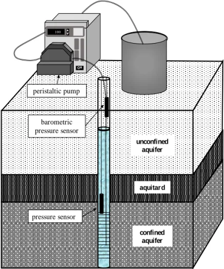
Des essais de perméabilité in situ ont été effectués dans des puits de surveillance installés dans des nappes captives situés dans trois sites d'essai. Le premier site est un système aquifère à échelle réduite construit en laboratoire, homogène et isotrope. Il a un volume de 3.05 m x 2.44 m x 1.22 m et se compose d'une nappe libre supérieure, sus-jacent à un aquitard, et d'une nappe captive dans le fond. Un nombre total de 24 MWs a été installé dans l'aquifère de sable à nappe captive, qui n'ont pas de filtre installé autour de la crépine. Le second site est situé à Sorel-Tracy avec une superficie de 150 m x 150 m, hétérogène avec des stratifications compliquées en profondeur. Un puits de pompage et 44 MWs ont été installés dans l'aquifère de sable à nappe captive de 3.5 m d'épaisseur. La distance moyenne entre deux MWs est de 30 m à l'exception de la zone autour du puits de pompage. Le troisième site est à Lachenaie, qui contient neuf sites
d'étude avec trois types de MWs installés à différentes profondeurs des strates. Les MWs testés ont pénétré dans l'aquifère de roche de schiste à nappe captive à une profondeur de plus de 6 m. Les essais CH, également connue sous le nom d’essais de débit constant, ont été effectués à l'aide d'une pompe péristaltique jusqu'à ce que le niveau d'eau dans le tuyau MW atteigne une stabilisation. Les essais VH ont débuté par le changement soudain d'un volume d'eau dans le tuyau et la réponse subséquente du niveau d'eau a été enregistrée dans le temps. La variation du niveau d'eau pendant les essais a été surveillée par une paire de transducteurs de pression absolue (PT) et de transducteur de pression atmosphérique (APT), qui sont des outils de surveillance plus précis et plus efficaces que d'autres outils de mesure. L'importance de l'étalonnage de PT seul a été bien reconnue, mais peu de chercheurs et de praticiens ont évalué l'importance de l'étalonnage et de la surveillance synchrone de la paire PT-APT. Les abaissements des essais CH et des différences de hauteur hydraulique des essais VH sont souvent obtenus par soustraction directe de la lecture courante PT (t) et du PT (pré-test) initial, ce qui revient à négliger la variation de pression d'air pendant l'essai.
Par conséquent, la thèse présente d'abord l'approche pour calibrer les transducteurs de pression sur le bureau des utilisateurs, afin d'évaluer leurs erreurs d'étalonnage systématiques. La paire PT-APT a ensuite été utilisée pour enregistrer les résultats d'essais CH et VH de courte durée dans 14 puits qui surveillaient la nappe captive à échelle réduite en laboratoire et un essai à niveau remontant de longue durée dans l'argile de Lachenaie. L'influence de la surveillance synchronisée pour la paire PT-APT, sur des données de test à court et à long terme a été quantifiée. Les résultats montrent que l'étalonnage doit être mis en œuvre pour chaque paire de PT et APT avant les essais in situ. A l'exception d'un test à charge variable très rapide, la fluctuation atmosphérique avec le temps joue un rôle important dans les résultats des essais, et donc le suivi synchronisé de la paire est nécessaire pour tous les essais.
Chaque essai de perméabilité in situ peut être réalisé avec un flux entrant de l'aquifère dans le MW ou sortant du MW vers l'aquifère, ce qui donne quatre types d'essais: les essais de décharge et d'injection (CH), et les essais à niveau montant et descendant (VH). Pour les MW parfaitement installés et développés, les mêmes valeurs de K devraient être données par des essais de deux écoulements opposés en raison de leurs mécanismes physiques identiques. Cependant, l'état de la crépine et du filtre peut empirer au fil du temps, après divers essais in situ et prélèvements d'eau
souterraine. Les théories ont été discutées précédemment mais les résultats pratiques des deux façons de conduire les essais CH et VH dans le même MW ont rarement été comparées par les praticiens. En outre, les gens comparaient et expliquaient rarement les deux méthodes d'essai communément utilisées: les essais de décharge et à niveau montant, et les essais d’injection et à niveau descendant du point de vue expérimental.
Dans la thèse, les essais d'injection et de décharge de type CH ont été effectués en injectant constamment de l'eau dans et en évacuant de l'eau à partir d'un seul MW, respectivement, pour générer une différence de charge hydraulique constante (état stationnaire). L’essai à niveau descendant a été effectué en ajoutant instantanément un volume d'eau, et pour un essai à niveau remontant, une écope ou une tige solide a été utilisée pour créer un déclin soudain du niveau d'eau. Tous les types d'essais ont été réalisés dans 33 puits de surveillance (MW) installés dans les trois sites. Les résultats des essais avec les flux entrants et sortants de divers cas indiquent des écarts dans les valeurs K pour le même MW. Bien que les MW aient été développés peu après leur installation, un certain colmatage de l'écran/du filtre ou de l'érosion interne du filtre/ du sol adjacent se produit pendant les essais. De plus, les K (essai CH), fréquemment inférieurs aux K (essai VH), sont considérés comme plus précis car l’essai CH implique un plus grand volume de sol et dure plus longtemps. Des recommandations pratiques ont également été fournies pour le choix de la méthode d'essai.
Dans certains cas de terrain, les praticiens n'ont pas accordé suffisamment d'attention au mécanisme de départ de l’essai VH: ils ont négligé le changement soudain de colonne d'eau et fait une analyse VH de la phase de récupération après une période de pompage relativement longue (essai CH). Les méthodes de Hvorslev et du graphique de vitesse, qui sont utilisées pour interpréter l’essai VH, ont été utilisées pour analyser ces données de récupération. L'application a donné deux résultats anormaux: (1) la forme du graphe de vitesse est dispersée ou courbe au lieu d'être droite, et (2) les valeurs KVH déterminées par les méthodes d'interprétation d’essai VH ne
sont pas équivalentes aux valeurs KCH par la méthode d'interprétation d’essai CH (solution de
Lefranc). La thèse a théoriquement prouvé que les méthodes d'interprétation pour l’essai VH sont applicables aux données de l’essai de récupération après un essai CH. Les anomalies dans le graphique de vitesse et les différences dans les valeurs KCH et KVH sont dues à une mauvaise
installation des MWs. Pour deux cas de MW bien installés, le diagramme de vitesse présentait des droites et les valeurs de KCH et KVH étaient très proches.
En variante, les essais de perméabilité in situ peuvent être réalisés de manière numérique, ce qui permet de visualiser et de quantifier les propriétés de l’écoulement et du flux au cours d'un essai à tout moment. Fréquemment, le rayon d'influence du MW est inconnu, ce qui entraîne des difficultés à définir la distance radiale limite R du modèle de l'aquifère. Une valeur R élevée peut ne pas être représentative car le taux de pompage pour un essai à CH dans des conditions de terrain est faible et le rayon d'influence sera donc faible. Cela augmente aussi considérablement le temps de calcul car le drainage non saturé prend beaucoup de temps. De plus, les facteurs de forme numérique (c) dans la littérature précédente ont été obtenus pour les conditions d'équilibre de l’essai CH seulement, et dans des conditions saturées uniquement, alors que les essais CH et VH sont effectués dans la pratique dans des zones saturées et parfois non saturées.
Ainsi, les moyens numériques pour simuler les essais CH et VH dans les nappes libres via le code d'éléments finis Seep/W ont été présentés, car les nappes libres présentent un fort potentiel de contamination. Les valeurs c ont été déduites numériquement en régime permanent et transitoire (soit pour un essai CH ou VH), en considérant l’écoulement non saturé de l'aquifère. L’essai CH a atteint l'état d'équilibre après une condition transitoire, qui a été simulée de deux façons: on a appliqué soit une différence de charge constante soit un débit constant comme condition aux limites de la crépine. L’essai VH était totalement en état transitoire. Deux séries de modèles d'aquifères équipés de MW ont été analysées et comparées; les MWs ont soit un filtre ou non. En outre, les influences de la distance radiale limite de la limite externe, les dimensions et les positions de la zone d'injection d'eau, et les types de matériaux aquifères sur les valeurs numériques c ont été étudiées. Les valeurs R représentatives pour chaque type de modèle d'essai ont également été déterminées.
ABSTRACT
Field permeability tests are easy to be performed in a single monitoring well (MW) and yield little disturbance to in-situ soil. The local K values in situ are obtained from two methods of field permeability tests, i.e., constant-head (CH) and variable-head (VH) tests. For homogeneous and isotropic aquifer layers, the average local values of K in several wells can be representative of the
K value of the soil because the scale effect is negligible. The theories of the test and interpretation
methods are mature; however, non-ideal field operations and poorly installed MWs may yield some errors, which greatly influence the test results. As a result, the derived K values are less accurate. Using inaccurate K values may affect the assessment in many practical problems like seepage and stability of dams, infiltration from disposal fields, contamination transport in groundwater etc. Therefore, the study focused on quantifying imperfect conditions which have not been discussed before and improving the reliability of the field permeability tests, in order to analytically, experimentally and numerically provide accurate assessments for the K value. The imperfections were caused by incorrect calibration and monitoring of pressure transducers, opposite directions of water flowing through the water injection zone, different test types and interpretation methods we used, and inappropriate numerical models.
Field permeability tests were conducted in monitoring wells installed in confined aquifers located in three test sites. The first site is a reduced-scale aquifer system built in the laboratory, which is homogeneous and isotropic. It has a volume of 3.05 m x 2.44 m x 1.22 m and consists of an upper unconfined aquifer, overlying an aquitard, and a confined aquifer in the bottom. A total number of 24 MWs were installed in the confined sand aquifer, which have no filter pack installed around the screen. The second site is located in Sorel-Tracy with an area of 150 m x 150 m, which is heterogeneous with complicated stratifications in depth. A pumping well and 44 MWs were installed in the confined sand aquifer of 3.5 m in thickness. The average distance between two MWs is 30 m except for the area around the pumping well. The third one is in Lachenaie, which contains nine study sites with 3 types of MWs installed at different depths in the strata. The tested MWs penetrated in the confined shale rock aquifer by a depth over 6 m. The CH tests, also known as constant flow rate tests, were performed using a peristaltic pump until the water level in the MW pipe reached stabilization. The VH tests were started by the sudden change of a volume of water in the pipe and the subsequent water level response was
recorded against time. The variation in water level during the tests was monitored by a pair of absolute pressure transducer (PT) and atmospheric pressure transducer (APT), which are more accurate and efficient monitoring tools compared to other measurement approaches. The importance of calibration of PT alone has been well recognized, however, few researchers and practitioners valued the importance of calibration and synchronous monitoring of the PT-APT pair. The drawdowns of the CH tests and hydraulic head differences of the VH tests are often obtained by the direct subtraction of current PT (t) and the initial PT (pre-test), which means that the variation in air pressure is neglected during the test.
Therefore, the thesis first presents the approach to calibrate the pressure transducers on users’ desk, in order to assess their systematic calibration errors. The PT-APT pair was then used to register test data during short-duration CH and VH tests performed in 14 wells monitoring the reduced-scale confined aquifer in the lab and a long-duration rising-head test in Lachenaie clay. The influence of synchronized monitoring for the PT-APT pair, on short- and long-term test data, was quantified. The results show that the calibration must be implemented for each pair of PT and APT before the field tests. Except for a very rapid variable-head test, the atmospheric fluctuation with time plays a significant role in the test results, and thus the synchronized monitoring of the pair is necessary for all tests.
Each test method of the field permeability tests can be carried out with either an inward flow from aquifer to pipe or outward flow from pipe to aquifer, which yields four test types: discharge and injection tests (CH), and rising- and falling-head tests (VH). For perfectly installed and developed MWs, same K values should be given by tests of two opposite flows due to their identical physical mechanisms. However, the condition of the well screen and filter pack may deteriorate over time, after various field tests and groundwater samplings. The theories were discussed previously but the practical results of the two ways to conduct the CH- and VH-tests have been rarely compared by the practitioners in the same MW. In addition, people rarely compared and explained the two commonly used test methods: discharge and rising-head tests, and injection and falling-head tests from the experimental aspect.
In the thesis, CH injection and discharge tests were performed by constantly injecting water into and discharging water from a single MW, respectively, to generate a constant hydraulic head difference (steady state). The falling-head test was conducted by instantaneously adding a volume
of water and for a rising-head test, a bailer or solid rod was used to create a sudden water level decline. All types of tests were conducted in 33 monitoring wells (MWs) installed in the three sites. The test results with inward and outward flows of various cases indicated discrepancies in
K values for the same MW. Although the MWs were developed soon after their installation, some
clogging of the screen/filter pack or internal erosion of the filter pack/adjacent soil occurs during the tests. Moreover, the K values (CH tests), frequently lower than the K values (VH tests), are considered to be more accurate because the CH test involves a larger soil volume and lasts longer. Some practical recommendations were also provided for the choice of test method.
In some field cases, the practitioners did not pay enough attention to the mechanism of the VH test: they neglected the sudden change in water column and considered the recovery phase after a relatively long pumping period (a CH test) as a VH test. The Hvorslev and velocity graph methods, which are used to interpret the VH test, were employed to analyze those recovery data. The application yielded two abnormal results: (1) the shape of the velocity graph is scattered or curved instead of being straight, and (2) the KVH values determined by the VH test interpretation
methods are not equivalent to the KCH values by the CH test interpretation method (Lefranc’s
solution). The thesis theoretically proved that the interpretation methods for the VH test are applicable to the CH recovery test data. The abnormality in velocity plot and discrepancies in
KCH and KVH values were found to be due to the poor installation of MWs. For two cases of MWs
in good conditions, the velocity plot presented straight lines and the values of KCH and KVH were
very close.
Alternatively, the field permeability tests can be performed in numerical ways, by which the seepage and flux properties during a test at any time may be visualized and quantified. Frequently, the influence radius of the MW is unknown, which causes difficulties in defining the boundary radial distance R of the aquifer model. A large R value may not be representative because the pumping rate for a CH test in field conditions is small and thus the influence radius will be small. It also greatly increases the computation time because unsaturated drainage takes a very long time. Additionally, the numerical shape factors (c) in previous literature were obtained for steady-state conditions of the CH test only, and for saturated conditions only, however, both CH and VH tests are performed in practice and for geometries with unsaturated seepage.
Thus, the numerical ways to simulate the CH and VH tests in unconfined aquifers via the finite element code Seep/W were presented, because the unconfined aquifers have a high potential for being contaminated. The c values were deduced numerically under steady- and transient-states (either for a CH or VH test), considering unsaturated seepage of the aquifer. The CH test reached steady-state after a transient condition, which was silumated in two ways: applied with either a constant head difference or a constant flow rate as the boundary condition of the screen. The VH test was totally in transient condition. Two series of aquifer models equipped with MWs were analyzed and compared; they either have a filter pack or not. Additionally, the influences of boundary radial distance of the external boundary, dimensions and positions of the water injection zone, and aquifer material types on the numerical c values were studied. The representative R values for each type of test model were also determined.
TABLE OF CONTENTS
DEDICATION ... III ACKNOWLEDGEMENTS ... IV RÉSUMÉ ... V ABSTRACT ... IX TABLE OF CONTENTS ... XIII LIST OF TABLES ... XVII LIST OF FIGURES ... XVIII LIST OF SYMBOLS AND ABBREVIATIONS... XXI
CHAPTER 1 INTRODUCTION ... 1
1.1 Context and motivation ... 1
1.2 Research question and objectives ... 4
1.3 Dissertation structure ... 5
CHAPTER 2 LITERATURE REVIEW ... 6
2.1 Pressure transducer calibration ... 6
2.2 In-situ tests for soil permeability ... 7
2.2.1 Aquifer tests ... 8
2.2.2 Field permeability tests ... 10
2.3 Field permeability test interpretation ... 12
2.3.1 Results of the field permeability test ... 12
2.3.2 Interpretation for constant-head test in granular soils ... 14
2.3.3 Interpretation for constant-head test in clay ... 24
2.3.4 Interpretation for variable-head test ... 27
2.4 Error sources in measurements of field permeability tests ... 42
2.5 Numerical code-Seep/W ... 45
2.5.1 Theory ... 45
2.5.2 Application ... 48
CHAPTER 3 ARTICLE 1: FIELD PERMEABILITY TESTS: IMPORTANCE OF CALIBRATION AND SYNCHRONOUS MONITORING FOR BAROMETRIC PRESSURE SENSORS ... 50
3.1 Introduction ... 51
3.2 Theory of interpretation methods ... 54
3.3 Test site description and materials ... 57
3.3.1 Large sand box installed with monitoring wells ... 57
3.3.2 Lachenaie clay site and monitoring wells ... 58
3.3.3 Pressure transducers ... 59
3.3.4 Other required apparatuses ... 60
3.4 PT-APT pair calibration and monitoring ... 60
3.5 In situ permeability test manipulation ... 61
3.6 Test results ... 62
3.6.1 Calibration of PT-APT pairs on user’s desk ... 62
3.6.2 Influence of barometric synchronous monitoring on in-situ tests ... 64
3.7 Summary ... 71
CHAPTER 4 ARTICLE 2: FIELD PERMEABILITY TESTS WITH INWARD AND OUTWARD FLOW IN CONFINED AQUIFER ... 74
4.1 Introduction ... 74
4.2 Interpretation methods ... 78
4.3.1 The sand box installed with monitoring wells ... 81
4.3.2 Sorel site installed with MWs ... 82
4.3.3 Lachenaie site installed with MWs ... 84
4.4 Field permeability tests manipulation ... 84
4.5 Field Permeability Test Results and Analysis ... 85
4.5.1 Shape factors ... 85
4.5.2 Large sand box ... 86
4.5.3 Sorel site ... 88
4.5.4 Lachenaie site ... 90
4.6 Comparison of Tests with Inward and Outward Flows ... 95
4.7 Comparison of CH and VH tests ... 98
4.8 Summary ... 101
CHAPTER 5 ARTICLE 3: PLAUSIBLE VARIABLE-HEAD TESTS INITIATED WITH CONTINUOUS PUMPING IN MONITORING WELLS ... 104
5.1 Introduction ... 104
5.2 Theoretical solutions ... 105
5.2.1 Interpretation of hydraulic conductivity ... 105
5.2.2 Theoretical examination ... 107
5.3 Examples of poorly installed wells ... 109
5.3.1 Example 1 ... 109 5.3.2 Example 2 ... 110 5.3.3 Example 3 ... 111 5.3.4 Example 4 ... 112 5.3.5 Example 5 ... 113 5.3.6 Discussion ... 114
5.4 EXAMPLES of good wells ... 115
5.4.1 Example 6 ... 115
5.4.2 Example 7 ... 116
5.5 Summary ... 117
CHAPTER 6 NUMERICAL VALUES OF SHAPE FACTORS FOR FIELD PERMEABILITY TESTS IN UNCONFINED AQUIFERS ... 120
6.1 Introduction ... 120
6.2 Field permeability tests modelisation ... 122
6.2.1 Unconfined aquifer models ... 122
6.2.2 K(u) and (u) functions ... 124
6.2.3 Boundaries for field permeability tests ... 128
6.3 Shape factors equations ... 128
6.4 Theoretical values of shape factors ... 130
6.5 Influences of the four variables on numerical shape factors ... 131
6.5.1 Boundary radial distance influence on shape factor ... 131
6.5.2 Water injection zone dimension and position influence on shape Factor ... 139
6.5.3 Material influence on numerical shape factors ... 141
6.6 Summary ... 146
CHAPTER 7 GENERAL DISCUSSION ... 149
CHAPTER 8 CONCLUSION AND RECOMMENDATIONS ... 157
8.1 Conclusion ... 157
8.2 Limitations and Recommendations ... 161
LIST OF TABLES
Table 3.1: Local hydraulic conductivities for MWs of the two types field permeability tests ... 69
Table 4.1: Summary of test types and numbers ... 78
Table 4.2 Useful parameters to calculate the hydraulic conductivities for the three sites ... 86
Table 4.3: Hydraulic conductivities from each MW of the confined aquifers in three sites ... 94
Table 5.1: Several information of the examples. ... 109
Table 5.2: Elements of comparison for the seven examples. ... 118
Table 6.1: Basic soil geotechnical and hydraulic parameters ... 125
Table 6.2: Theoretical shape factors ... 131
LIST OF FIGURES
Figure 2.1: Schematic of pumping tests ... 9
Figure 2.2: Two ways to conduct the CH test ... 11
Figure 2.3: Examples of test results of constant-head tests ... 13
Figure 2.4: Example of test result of a variable-head test (from ISO 22282-2 2012) ... 13
Figure 2.5: Infiltrated water amount depending on the pressure difference ... 15
Figure 2.6: The relative velocity curve ... 19
Figure 2.7: The time-drawdown plot ... 23
Figure 2.8: Definitions of variables in pumping and recovery phases ... 23
Figure 2.9 The schematic of sphere piezometer in clay ... 24
Figure 2.10: Variation of pore water pressure with time around an ideal spherical cavity ... 26
Figure 2.11: Functions of and . ... 29
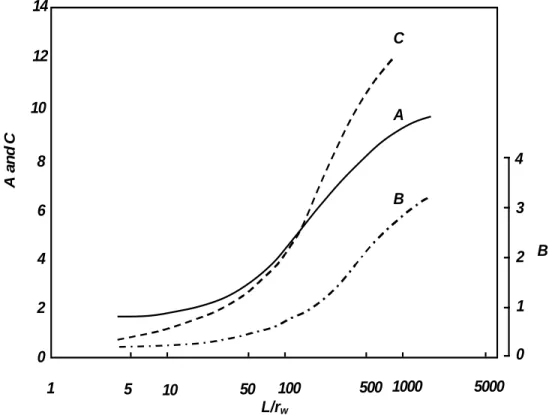
Figure 2.12: Graph of the coefficient A, B, and C versus L/rw for the Bouwer and Rice equation (1976) ... 32
Figure 2.13: Curved semi-log graphs (from Chapuis, 2015). ... 33
Figure 2.14: Velocity graph ... 34
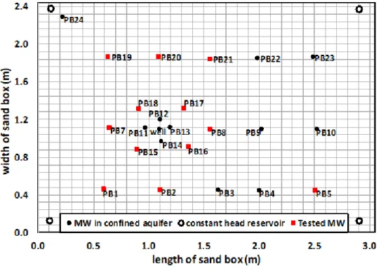
Figure 3.1: Plan of monitoring wells (MWs) installed in the sand box. ... 58
Figure 3.2: Pressure transducer principles. ... 59
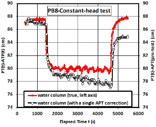
Figure 3.3: Example of [PT(t) – APT(t)]air data for a pair of transducers. ... 63
Figure 3.4: Influence of f barometric pressure fluctuation on constant-head test. ... 64
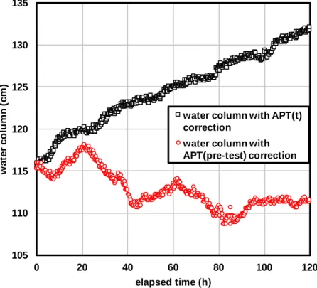
Figure 3.5: Five days of PT and APT data for the rising-head test in Lachenaie clay. ... 66
Figure 3.6: Influence of barometric pressure fluctuation on long-term rising-head test data. ... 67
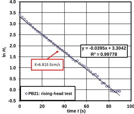
Figure 3.7: Semi-log graph of a rising-head test in PB21 ... 68
Figure 3.8: Analysis of the distribution of the K values obtained with the variable-head and constant-head tests performed in 14 monitoring wells of the large sand box. ... 70
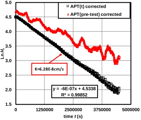
Figure 3.9: Semi-log graph of the rising-head test in Lachenaie clay ... 71
Figure 4.1: Schematic of the CH test in MW installed in the sand tank. ... 82
Figure 4.2 Plan view of the Sorel site. ... 83
Figure 4.3: Influence of impervious boundary on CH discharge test in PB1. ... 87
Figure 4.4: Two types of CH test results in MW (30,10). ... 88
Figure 4.5: Two types of VH test results in MW (30,10). ... 89
Figure 4.6: Two types of CH test results in site 1. ... 90
Figure 4.7: Time-drawdown interpretation of discharge test site 1. ... 91
Figure 4.8: Two types of VH test results in Lachenaie site 2. ... 92
Figure 4.9: Two types of VH test results in site 9 ... 93
Figure 4.10: The K comparison of tests with outward and inward flows in the sand box. ... 95
Figure 4.11: The K comparison of tests with outward and inward flows in Sorel ... 96
Figure 4.12: The K (m/s) comparison of VH and CH tests in sand box ... 99
Figure 4.13: The K (m/s) comparison of VH and CH tests in Sorel ... 100
Figure 4.14: The sketch of created filter zone ... 100
Figure 5.1: Example 1 in sand, L = 225 cm, D = 11.4 cm ... 110
Figure 5.2: Example 2 in sand, L = 360 cm, D = 11.4 cm ... 111
Figure 5.3: Example 3 in sand, L = 298 cm, D=11.4 cm ... 112
Figure 5.4: Example 4 in till, L = 367 cm, D = 10.16 cm ... 113
Figure 5.5: Example 5 in till, L = 367 cm, D = 10.16 cm ... 114
Figure 5.6: Example 6 in sand, L = 114 cm, D = 9 cm. ... 116
Figure 5.7: Example 7, L = 100 cm, D = 15.24 cm. ... 117
Figure 6.1: Different lengths and positions of two series of water injection zones. ... 123
Figure 6.3: Corresponding K(u) functions of aquifer materials. ... 127
Figure 6.4: Shape factors versus boundary radial distance (no filter pack). ... 132
Figure 6.5: Examples of variation of the hydraulic head versus distance. ... 133
Figure 6.6: CH steady and transient water tables at r = 0.03 m versus boundary radial distance. . 133
Figure 6.7: Shape factors versus boundary radial distances (with a filter pack). ... 134
Figure 6.8: CH steady and transient water table at r = 0.0762 m (interface between soil and filter pack) versus boundary radial distance R ... 135
Figure 6.9: Flow rate Q variations in pipe with CH test time t in linear and log scale. ... 136
Figure 6.10: Hydraulic head H variations in pipe with CH test time t. ... 137
Figure 6.11: CH test times by two simulating methods versus boundary radial distances. ... 138
Figure 6.12: Percentage differences between theoretical and numerical shape factors versus boundary radial distances (no filter pack). ... 138
Figure 6.13: Shape factors with regard to different injection zones (no filter pack). ... 140
Figure 6.14: Shape factors with regard to different injection zones (with a filter pack). ... 141
Figure 6.15: Theoretical and numerical shape factors with regard to different materials. ... 142
Figure 6.16: Theoretical and numerical shape factors with regard to different materials. ... 143
Figure 6.17: Relationship between saturated hydraulic conductivities and CH test time (1st series). ... 144
Figure 6.18: Relationship between saturated hydraulic conductivities and VH test time. ... 145
LIST OF SYMBOLS AND ABBREVIATIONS
a Constant
A Summation over the area of an element
A Dimensionless coefficient determined by a function of L/rw
APT Atmospheric pressure transducer
b Thickness of confined aquifer, saturated thickness of unconfined aquifer (m)
b Constant
B Dimensionless coefficient determined by a function of L/rw
[B] Gradient matrix
c shape factor (cm or m)
C Coefficient of consolidation, parameter equals Sinj/c.
[C] Element hydraulic conductivity matrix
C Dimensionless coefficient determined by a function of L/rw
CU Coefficient of uniformity
CH Constant-head
d Diameter of MW pipe/borehole casing, distance from water level to the bottom of the water injection zone (mm or cm)
d10 Effective size/ size at 10% passing (cm)
d60 Size at 60% passing (cm)
D Diameter of the cavity/water injection zone (cm)
Da Average diameter of the tapered cavity/water injection zone (cm)
e Void ratio
f Slope
H Apparent hydraulic head difference, mean head difference of two consecutive measurements (cm or m)
{H} Vector of nodal heads dH, H Increment of head difference
H1, H2, H3 Three different applied hydraulic head difference
Hc Constant hydraulic head difference between the initial and stabilized piezometric
levels in the well, applied hydraulic head (m)
He Head at end of time increment (m)
Hi Initial hydraulic head difference, head at the initiation of time increment (cm or m)
H0 Piezometric error (cm or m)
Hj,Hj+1 Two consecutive head difference measurements (cm or m)
Hp Limit of hydraulic head difference (m)
Hr Real hydraulic head difference (cm or m)
K Hydraulic conductivity (cm/s or m/s) [K] Element characteristic matrix
K1 Hydraulic conductivity of the screen (m/s)
K2 Hydraulic conductivity of the filter materials (m/s)
K23 Hydraulic conductivity of the created filter zone (m/s)
K3 Hydraulic conductivity of the soil (m/s)
Ksat Saturated hydraulic conductivity (cm/s or m/s)
KCH Hydraulic conductivity calculated by the interpretation method of CH test
(Lefranc’s solution) (m/s)
KVH Hydraulic conductivity calculated by the interpretation methods of VH test (m/s)
KVH2 Hydraulic conductivity calculated by the velocity graph method with the entire
velocity plot (m/s)
KVH2’ Hydraulic conductivity calculated by the velocity graph method with the straight
portion of velocity plot (m/s)
KVH3 Hydraulic conductivity calculated by the optimized semi-log graph method (m/s)
L Length of cavity/water injection zone, summation over the edge of an element (cm or m)
mw Slope of versus uw:
[M] Element mass matrix MW Monitoring well
<N> Vector of interpolation function
P, P1, P2 Slope
PL Piezometric level
PT Pressure transducer
Q Constant pumping/discharge/injection flow rate, steady-state outflow rate (m3/s) {Q} Element applied flux vector
Qe Nodal flux at end of the time increment (m3/s)
Qinj Water flow rate into the pipe/borehole casing (m3/s)
Qs, Qsoil Water flow rate through the injection zone/soil (m3/s)
r Distance from the center of pumping well to the center MW or piezometer (m)
r1, r2 Distance from the center of pumping well to the center of MW1 and MW2 (m)
rc Radius of MW pipe/borehole casing (cm)
rw Radius of cavity/water injection zone (cm)
R Boundary radial distance (m)
s Drawdown (m)
s1, s2 Drawdowns in MW1 and MW2 (m)
s Drawdown difference per log cycle of t (m)
s’ Residual drawdown (m)
s’ Residual drawdown difference per log cycle of t/t’ (m)
S Storativity, surface area of the injection zone
Sinj Cross-sectional area of MW pipe/borehole casing (cm2)
Ss Specific storativity
t Elapsed time (s)
tj,tj+1 Two consecutive time measurements (s)
dt, t Increment of time (s)
t’ Time from the beginning of recovery test (s)
ti Initial time (s)
T Transmissivity (m2/s), time factor
u, uw Pore water pressure (kPa)
u Excess pore water pressure (kPa)
ui Initial pore water pressure (kPa)
v Relative velocity calculated by two consecutive measurements (m/s)
V Steady-state outflow volume (m3)
VH Variable-head
W(u) Well function of pumping period W(u’) Well function of residual period
z Elevation (m)
Volumetric water content
w Unit weight of water (kN/m3)
Ratio of horizontal and vertical hydraulic conductivities, storage term for a transient seepage equals to mw
CHAPTER 1
INTRODUCTION
1.1 Context and motivation
Hydraulic conductivity, K, represents the ability of water moving through porous materials (Todd and Mays, 2005). Three ways including empirical approaches, laboratory experiments, and in-situ tests are normally used to obtain the saturated K value. To estimate the hydraulic conductivity empirically, many predictive equations were proposed based on the grain size distribution, porosity and other properties of the soil, reviewed by Chapuis (2012a). In the laboratory, the saturated K values of granular soils can be determined with either a constant or falling head test in a rigid-wall or flexible-wall (triaxial cell) permeameter. The detailed specifications are included in ASTM standards (ASTM D2434, 2006; ASTM D5084, 2016). The pumping and field permeability tests are performed to evaluate the in-situ K values.
Knowledge of the in-situ K values of aquifers is critical for many hydrogeological, geotechnical, and environmental problems, such as seepage through dams and their foundations, infiltration from disposal fields, and monitoring groundwater contamination (Chapuis, Soulié and Sayegh, 1990). Pumping test is considered to be the most reliable test to estimate the hydraulic conductivity due to its slightest disturbance in soil properties in the field (Todd and Mays, 2005). It is performed by constantly discharging a pumping well and observing the water level in the controlled well and several piezometers at different distances (e.g., Chapuis 1999a; Kruseman and Ridder, 1994). However, a pumping test is not always justified or even possible. If there is only a single monitoring well (MW), piezometer or borehole casing, the local hydraulic conductivity may be determined by field permeability tests of constant-head (CH) and variable-head (VH). The K values assessed by different types of tests may provide different values due to the scale effect. For homogeneous aquifer, however, the scale effect is insignificant and can be neglected (Chapuis et al., 2005a; Dallaire, 2004).
The research focuses on the field permeability tests in monitoring wells (MWs), which is easier to be achieved than the pumping test. Although the theories of the tests are well developed, the field manipulation details can significantly affect test results (Canadian Geotechnical Society, 1985; Chapuis et al., 1990; Milligan, 1975). Thus, the research dedicates effort to studying the
effects of several error sources on the derived hydraulic conductivities and providing practical recommendations to improve the reliability of the field permeability tests.
CH and VH tests were conducted in the monitoring wells installed in a large sand box (a reduced-scale aquifer system) and two field sites in Sorel and Lachenaie. All tests were conducted with two opposite water flows. The water flowing from aquifer to well pipe was defined an inward flow, caused by a water withdrawal from the MW. The injection of water into the pipe generates an outward water flow from pipe to aquifer. The screens of the MW pipe are located in the confined aquifer layer, where the pore water pressure is greater than the atmospheric pressure. The water level position versus time during a test is registered by an absolute pressure transducer (PT) and an atmospheric pressure transducer (APT). The PT measures the total pressure acting on its sensor, including the water column and atmospheric pressure above the sensor. To obtain the true water column height above the sensor, the barometric pressure obtained by an APT should be subtracted from the PT reading. The transducer converts water or barometric pressure into a height of water column, and the built-in datalogger outputs the registered data in the unit of cm directly.
The calibration method for different PT-APT pairs is firstly proposed, to assess their accuracy. The influence of the variations in barometric pressure on the derived K value during short-term tests in a sand aquifer is then examined. Additionally, the influence on the recovery of a long-term rising-head test in clay is analyzed.
The CH tests were performed by discharging or injecting a single constant flow rate from or into the riser pipe until the water level reaches stabilization. After shutting off the pump, the water level in the riser pipe slowly returned to the pre-test static water level. The pumping rates were automatically controlled by the peristaltic pump and monitored using a burette and a stopwatch during the test. The CH tests with outward and inward water flows were termed injection and discharge tests, respectively. Water-level rises and drawdowns were registered by a pair of PT and APT every 15 seconds.
Compared to the continuously constant water flow, the VH tests (slug tests), were initiated with a sudden change of water volume in the pipe by a quick addition (falling-head) or removal (rising-head) of water, and the subsequent water level response was recorded over time. However, some practitioners were not aware of this “sudden” water level change. They considered the recovery
period after a long-time groundwater sampling/discharging (CH test) as a VH test and employed the interpretation methods of VH tests to analyze the recovery test data. The abnormalities in test plots aroused our interest. Therefore, K values interpreted by CH and VH solutions were compared, where the discrepancies indicate a poor installation of MW. Moreover, the connections between the interpretation approaches for VH and CH tests were explained.
In the project, the falling-head test was conducted by quickly adding a volume of water. The rising-head test was started with a solid rod in the reduced-scale sand aquifer and Sorel site, and a bailer in Lachenaie site. The PT and APT were synchronized to take readings with a 2-second interval.
The theories of the field permeability test method have been well-developed. The CH test data were interpreted by the Lefranc’s solution (CAN/BNQ 250-135, 2014) to obtain the local K values, which may be different from the hydraulic conductivity in a large scale (AFNOR NF P94-132, 2000). The time-drawdown method (Cooper and Jacob, 1946) was used to interpret the transient state of the CH test for which equilibrium had not been reached. The VH test data were interpreted using the semi-log graph method (Hvorslev, 1951). If the semi-log plot is curved, the piezometric correction must be made by the velocity graph method (Chapuis, Paré and Lavallée, 1981) or the Z-t method (Chiasson, 2005, 2012). The K values obtained from different tests and interpretation methods were compared and discussed.
Theoretically, injection and discharge tests should provide close K values, so do falling- and rising-head tests, because the manipulations and physical mechanisms of each two types of the tests are identical except that the water flow directions are opposite. If sediments at the bottom of the pipe are carried by an outward flow, clogging of the well screen may occur and thereby decrease the permeability of soil. Also, erosion may appear in the gravel pack resulting from an inward flow that carries fine particles, and hence a higher K value is attained. To check the possibility of these situations, the tests with opposite flows were conducted in succession, and the
K values were compared.
The two types of field permeability tests in unconfined aquifers were modelled with the finite element code Seep/W, to study the seepage property and numerical values of shape factors, c, in the target aquifer. The code solves the seepage and conservation equations based on functions related to the pore water pressure. The models are axisymmetric, where the soil, filter material,
and pipe are homogeneous and isotropic. The unsaturated portions were fully defined for all materials. The lower boundaries of the unconfined aquifers were impervious, and the screen and far boundary conditions were specified for various cases.
The numerical simulation of CH tests was achieved in two ways, to apply either a constant head difference or a constant flow rate on the screen. The steady-state and transient analyses of the CH test were studied, whereas the entire VH test was in the transient state. Four variables including 11 boundary radial distances, 15 different soils properties, 4 different lengths of water injection zones, 3 different positions for the water injection zones were analyzed, to study their influences on the c values derived from the numerical CH and VH tests. Additionally, numerical c values were compared with the theoretical ones.
1.2 Research question and objectives
Despite the development, all field operations yield not-so-perfect conditions. If the monitoring wells or the field operations are not perfect, the hydraulic conductivity obtained is less accurate. The imperfections like hydraulic fractures, hydraulic short circuits, clogging, piezometric errors, selection of shape factors, etc. contribute to the inaccurate estimation of hydraulic properties of the aquifer. In addition, the errors caused by pressure transducers, opposite directions of water flows, different test types and interpretation methods may affect the reliability of test results. Therefore, it is essential to check these errors and remove or minimize them, in order to improve the reliability of field permeability tests.
The research is a continuous improvement to previous research on the reliability of the field permeability tests. It aims to study and quantify non-ideal conditions that have not been discussed and to provide practical recommendations and accurate assessments for the hydraulic parameters from experimental, analytical and numerical aspects.
To achieve the goal, several specific objectives are listed as follows,
1. Remove the systematic error caused by barometric variation during the test by calibrating and synchronously monitoring each PT-APT pair.
2. Examine how the PT-APT calibration and synchronous monitoring, during a test, influences the test data accuracy and the resulting K value.
3. Check the conditions of the screen and filter pack by conducting the field permeability tests of two opposite flows (i.e., rising- and falling-head tests, discharge and injection tests) in each MW. 5. Find the reason for the discrepancy of K values between CH and VH tests in the same MW by studying the connection of the interpretation methods of the two types of tests.
4. Verify the reliability of field hydraulic conductivity by comparing the results of CH and VH tests and provide practical recomendations for the choice of test method.
6. Simulate the CH and VH tests via numerical code, through which numerical values of shape factors of various cases are evaluated and the proper boundary radial distance of the aquifer model are determined.
1.3 Dissertation structure
The dissertation consists of seven chapters. Chapter 1 introduced the background of the research, based on which the objectives were proposed. Chapter 2 will present a critical review of previous work most related to the research. Chapter 3 will be devoted mainly to the description of the influence of barometric calibration and PT pair monitoring on the field permeability tests. Chapter 4 will compare CH and VH tests with two opposite flow directions in the confined aquifers of three different sites, which indicates the condition of screen clogging and filter pack erosion. Chapter 5 will provide theoretical and experimental evidence of the application of VH interpretation methods on the CH recovery tests. Chapter 6 will focus on the assessment of numerical shape factors under various conditions via the numerical code. Chapter 7 will provide a general discussion on the results. The last Chapter 8 will draw a conclusion for the entire study and discuss the limitations to provide useful inspirations for future research.
CHAPTER 2
LITERATURE REVIEW
2.1 Pressure transducer calibration
The three major types of sensors to gauge the water level in wells were sorted as float recorders, pressure transducers, and acoustic devices (Ritchey, 1986). Due to the limitation of traditional water level measuring devices (floats and acoustic devices) in small diameter (≤ 10 cm) wells, the potential of the application of electrical pressure transducers in water level measurement was initially proposed by Shuter and Johnson (1961). Afterwards, different types of pressure transducers based on the electrical method were designed and evaluated by researchers (e.g., Clark, Germond and Bennett, 1983; Holbo, Harr and Hyde, 1975; MacVicar and Walter, 1984; Keeland, Dowd and Hardegree,1997), in order to determine the pressure on the submerged stationary probe. Combined with electronic data recorders, the pressure transducers have been developed to be capable of collecting continuous water level or pressure data from wells (Freeman et al., 2004). A pressure transducer linked to a data logger or display device can be used in an aquifer test in the open well and is necessary for the test in a closed well where manual measuring method is unable to provide frequent measurements (ASTM D4044, 2015). It provides rapid measurements of water-level variations and can be programmed to register at different frequencies.
Down and Williams (1989) mentioned that if individual calibration for the pressure transducer is not carried out, large measurement errors will occur due to the unique response characteristics of each transducer. Their datalogger gave voltage outputs for the soil suction measurements. The calibration curve was plotted as suction versus millivolt sensor output, which is a linear response with a correlation coefficient of 1.0. The similar calibration process was implemented in the laboratory by Keeland et al. (1997) for the measurements of water levels in wells. The laboratory and field calibrations displayed straight calibration lines with correlation coefficients close to 1.0. Freeman et al. (2004) and ISO (2009) established guides on selection, installation, and operation of the submersible pressure transducers. Freeman et al. (2004) introduced various types of pressure transducers, used in wells, piezometers, soil-moisture tensiometers, and surface water gages, in the application of water resources. They pointed out the source of errors in commonly-used linear calibrations and proposed a temperature-corrected transducer calibration which
reduces residual error to 0.03% of full-scale output or less. It was suggested that users should recalibrate the PTs and determine their performance before exploiting them in the field. ISO (2009) specified in the scope of automated pressure transducer methods in measuring the water level in a well based on the work of Freeman et al. (2004). The calibration procedure for the individual pressure transducer is the same as previously mentioned.
For an absolute pressure transducer used in field permeability test, the real water column is the subtraction of barometric pressure from the total pressure measured. The necessity of calibration of individual pressure transducers was well recognized. ASTM D4050 (2014) regulated that the single pressure sensor should be checked before using in the field by raising and lowering a measured distance in the well. Meanwhile, the verification of the sensor readings periodically with a steel tape is required. However, little literature valued the significance of barometric pressure in the calibration process of the pressure transducer. Chapuis (2009a) indicated that atmospheric pressure is one of the reasons to affect the accuracy of the readings of pressure sensors. The noteworthy variations in barometric pressure have been mentioned in the test of checking accuracy and drift properties of pressure transducers, and it was pointed out that an industry-wide standard should be developed (Sorensen and Butcher, 2011). Zhang, Chapuis and Marefat (2015, 2018a) used field permeability test data in sand and clay to show the important influence of calibration and synchronous monitoring of atmospheric pressure on the water level measurements.
2.2 In-situ tests for soil permeability
In situ, the field permeability tests in a single well, piezometer, or borehole casing (AFNOR NF P94-132, 1992; ASTM D4044, 2015; CAN/BNQ 2501-135, 2501-130, 2014; ISO 22282-2, 2012) yield the local hydraulic conductivity, K. On a larger scale, the hydraulic parameters of transmissivity T and storativity S are determined by a pumping test, where a pumping well and several piezometers/ monitoring wells are needed to measure the water levels (Chapuis, 1999a; Kruseman, 1994; Todd and Mays, 2005). Compared to the laboratory tests, in-situ or field tests for soil permeability involve a larger soil volume and consider the macrostructure effects better (Olson and Daniel, 1981). As a result, they are preferred for saturated soils. In-situ tests for permeability were classified in several different ways, and the same test may have altered names. They are summarized herein to avoid confusing the readers.
2.2.1 Aquifer tests
The pumping and slug tests are collectively called aquifer test in textbooks of hydrogeology (Fetter, 2001; Istok and Dawson, 1991). The term “aquifer test”, in a narrow sense, refers in particular to the pumping test. In pumping tests, groundwater is either pumped into or from the pumping well at a constant flow rate, which corresponds to an injection or withdrawal test (ASTM D4050, 2014), shown in Figure 2.1a and b. When the pump is stopped, the water levels in the pumping well and piezometers start to return to the original water levels before the test, which is a recovery test. It provides reliable test data and examines the results of the pumping test independently (Kruseman, 1994). If the pumping rate is increased periodically, it is a step-drawdown test, which is able to assess the well performance (Istok and Dawson, 1991; Kruseman 1994) and evaluate the hydraulic conductivity when each step reaches equilibrium (Zhang et al., 2015).
The slug test, as its name suggests, is performed by abruptly adding or removing of a slug of water in a single injection or withdrawal well and water levels in the well are monitored subsequently, which corresponds to the slug injection and withdrawal test, respectively (Istok and Dawson, 1991). The sudden change of water volume can also be achieved by quick insertion or removal of a mechanical “slug,” or rapid increase or decrease of air pressure in the well (Chapuis, 2012b). Several ways to initiate a slug test were discussed in ASTM D4044 (2015). The slug test has overdamped or underdamped responses of water level, depending on the water mass in the well and the hydraulic properties of the aquifer (Van der Kamp, 1976). In overdamped cases (Chapuis, 1998; Cooper, Bredehoeft and Papadopulos, 1967; Hvorslev, 1951), the water level returns to equilibrium in an approximately exponential way after slugging. If the water level oscillates around the equilibrium level, the test is underdamped, which yields transmissivity and storativity (Kipp, 1985; Ross, 1985; Uffink, 1984; Van der Kamp, 1976) or only K values (McElwee, 2001; McElwee and Zenner, 1998; Zurbuchen, Zlotnik and Butler, 2002). The slug test was also called variable-head (VH) test in geotechnical engineering (e.g., Cassan, 2005; Chapuis, 1999b; Chapuis and Chenaf, 2003a; Monnet, 2015; Reynolds, 2015).
confined aquifer unconfined aquifer MW1 MW2 withdrawal well Q
initial piezometric level
rc r1 r2 aquitard impervious bed s s1 s2 ground surface
(a) withdrawal test
confined aquifer unconfined aquifer MW1 MW2 injection well Q
initial piezometric level
rc r1 r2 aquitard impervious bed s s1 s2 ground surface (b) injection test
Figure 2.1: Schematic of pumping tests
For the tight formations that have very low permeabilities, the duration of pumping test is inordinately long. The slug test was suggested and its duration can be shortened by using a pipe
of small radius (Bredehoeft and Papadopulos, 1980). However, the radius will be too small to put into practice if the permeability of the formation is extremely low, like the tightly compacted clays, shales, basalts, and salt formations that are used for the disposal of hazardous wastes. Several modified slug test methods were provided to shorten the test duration by pressurizing a volume of water into the formation (Bredehoeft and Papadopulos, 1980; Neuzil, 1982).
2.2.2 Field permeability tests
The constant-head (CH) and variable-head (VH) tests in casing borehole were first proposed by the French civil engineer Lefranc (1936, 1937), known as the Lefranc test. It is a reliable test method to obtain the local K value when the pumping test is not available for homogeneous and isotropic aquifers (Houti’s course note), included in several textbooks (Cassan, 1980, 2005; Monnet, 2015) and the French, International and Canadian standards (AFNOR NF P94-132, 1992, 2000; CAN/BNQ 2501-135, 2014; ISO 22282-2, 2012). It was also used to assess the groutability of the soil ground (Bell, 2004; Cambefort, 1987) and the anisotropy coefficient of the aquifer (Cassan, 2000; Lafhaj and Shahrour, 2004).
The test consists of generating a water flow with a constant or variable water head into a cavity of a given shape, named lantern, at the bottom of a borehole and observing the variations of the water level (Cassan, 2005). Three methods of the Lefranc test were described in the Canadian standard (CAN/BNQ 2501-135, 2014): 1) the constant-head test; 2) the variable falling-head test; 3) the variable rising-head test. The first way to conduct a constant-head (CH) test is to add or remove water continuously to maintain a constant water level in the well casing until the flow rate becomes nearly constant (Cassan, 2005; Monnet, 2015). It is easier to do the test with a constant flow rate, which is the second way to achieve a constant head difference, sometimes also called a constant-rate test (Cassan, 2005; ISO 22282-2, 2012). The two ways of the CH test are presented in Figures 2.2a, b. The CH tests of injecting and discharging at a constant rate until an equilibrium is reached were named CH injection and discharge tests (Zhang, Chapuis and Marefat, 2018b). The variable-head (VH) test herein is equivalent to the previously mentioned slug test initiated by filling or removing the water in the drill casing. The falling- and rising-head tests refer to slug-injection (baildown or slug-out) and slug-withdrawal (slug-in) tests, respectively. The variable-head test was not applicable in highly pervious formations in previous
times because the test is so fast that manual measurements may be impossible to take. With the pressure transducer, which is able to record with 0.5s intervals, the test is achievable.
Besides the borehole casing (Chapuis, 2001; Chapuis and Chenaf, 2003a), the CH and VH test methods could also be applied in driven permeameters (Chapuis and Chenaf, 2010), monitoring wells/piezometers (e.g., Chapuis, 1998; Zhang et al., 2018a, b), or double-packer permeameters (Mathias and Butler, 2007). The water of tests in driven casing seeps through either the end of the drill casing (CAN/BNQ 2501-130, 2014) or the cylindrical gravel pack below the driving shoe (CAN/BNQ 2501-135, 2014). They were collectively named the field permeability tests. Compared to the aquifer pumping test, the implementation of the CH test is faster and necessary equipment is reduced, and the test can be done as the geotechnical investigation progresses. However, it is less popular, which may be because that it has not been standardized in the US.
confined aquifer unconfined aquifer borehole casing inflow rc D aquitard impervious bed Hc ground surface
initial piezometric level
cavity (lantern) casing L outflow Q confined aquifer unconfined aquifer borehole casing constant Q rc D aquitard impervious bed Hc ground surface
initial piezometric level piezometric level at equilibrium state cavity (lantern) casing pump L
(a) maintain a constant hydraulic head (b) inject water at a constant rate
until reach a steady-state flow until reach a constant head (constant-flow test)
2.3 Field permeability test interpretation
2.3.1 Results of the field permeability test
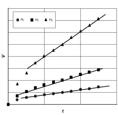
ISO 22282-2 (2012) illustrated three examples of the test results for the CH tests conducted in two ways and the VH tests. Figure 2.3 (a) presents the results of a CH test performed with a water injection at a constant flow rate. After some time, the hydraulic head of the test stabilizes. In fact, when injecting, there is a fairly rapid variation in the head while the water has not yet begun to permeate into the soil. Then the flow remains constant gradually, and the head increases or decreases regularly to stabilize at a level so that the flow through the wall of the cavity is equal to the injected flow, which indicates that steady state is reached (Cassan, 2005). If the CH test is conducted by discharging water constantly, the plot will have a constant drawdown instead of the rising water head. Figure 2.3 (b) displays three plots of CH tests conducted by applying three different constant hydraulic heads. The volume of water supplied or extracted are registered against time until the steady-state flow is achieved. The flow rate, the slope of the V-t curve, becomes constant after some variations. The VH test results are given in Figure 2.4, which refers to a falling-head test because the hydraulic head is decreasing with time. The head of a variable rising-head test increases with time.
H
t
13
t
V
7.3 Constant head test method
The results of a constant head test are the changes of volume or rate of water flow versus time (Figure 5).
Figure 7 — Example of test results of a constant head test for different hydraulic heads (multi-step test) (h3> h2> h1)
8 Reports
8.1 Field report
8.1.1 General
At the project site, a field report shall be completed. This field report shall consist of the following, if applicable:
a) summary log according to ISO 22475-1;
b) drilling record according to ISO 22475-1;
c) sampling record according to ISO 22475-1;
d) calibration record according to ISO 22282-1;
e) record of measured values and test results according to 8.1.2.
All field investigations shall be reported such that third persons are able to check and understand the results.
8.1.2 Record of measured values and test results
The record of measured values and test results shall contain the following data, if applicable (see Annex A).
a) General information:
1) name of the enterprise performing the test;
2) reference to this International Standard, e.g. ISO 22282-2:2012;
3) name of the client;
© ISO 2012 – All rights reserved 11
H1 H2 H2
(b) constant-head tests by maintaining three constant hydraulic heads (from ISO 22282-2 2012)
Figure 2.3: Examples of test results of constant-head tests
H
t
2.3.2 Interpretation for constant-head test in granular soils
2.3.2.1 Lefranc’s solution
The solution of the CH test at steady state was given by Lefranc (1936, 1937), which was referred by many researchers (e.g., United States Bureau of Reclamation, 1960, 1990; Benabdallah, 2010; Cassan 1980, 2000, 2005; Chapuis, 1999b, Chapuis et al. 1990; Dhouib et al., 1998; Lafhaj, 1998; Lafhaj and Shahrour 2002a, 2006; Rat, Laviron and Jorez, 1970) and normalized in several standards (AFNOR NF P94-132, 2000; CAN/BNQ 2501-135, 2014; ISO 22282-2, 2012).
The general equation of the field permeability test in steady state is similar to Darcy's, expressed as
c
s cKH
Q
Q (2.1)
where Q is the constant flow rate for the CH test that injects or discharges at a constant rate (Figure 2.2b), equal to the flow rate of water through the injection zone Qs when the test reaches
equilibrium, c is the shape factor, and Hc is the constant head difference between the initial and
stabilized piezometric levels in the well.
The saturated hydraulic conductivity is then determined:
c
cH Q
K (2.2)
For the CH test that maintains a constant water level, the steady-state outflow rate Q (Figure 2.2a) can be calculated by the steady-state outflow volume V and the corresponding elapsed time
t:
t V
Q (2.3)
The Equation 2.2 can be rewritten as:
t cH V K c (2.4)
2.3.2.2 ISO 22282-2 method
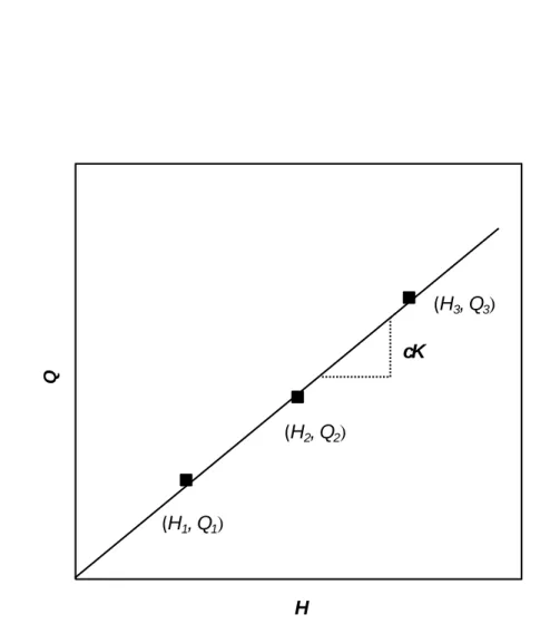
The constant-head test can be repeated at different hydraulic heads, for example, H1, H2, and H3.
Three constant flow rates are reached as a result. If the test is perfect, the plot of constant flow rates and their corresponding head differences is linear (Figure 2.5). The slope P can be used to calculate the hydraulic conductivity.
cK P (2.5) c P K (2.6) Q H (H1, Q1) (H2, Q2) (H3, Q3) cK
Figure 2.5: Infiltrated water amount depending on the pressure difference 2.3.2.3 Theoretical curve method
According to Cassan (2005), the transient phases including the injection/discharge and recovery of the CH test with a constant flow rate can also be interpreted.