UNIVERSITÉ DE MONTRÉAL
DESIGN AND IMPLEMENTATION OF A FUZZY CONTROLLER FOR STEERING MICROPARTICLES INSIDE BLOOD VESSELS BY USING A MRI SYSTEM
KE PENG
DÉPARTEMENT DE GÉNIE INFORMATIQUE ET GÉNIE LOGICIEL ÉCOLE POLYTECHNIQUE DE MONTRÉAL
MÉMOIRE PRÉSENTÉ EN VUE DE L’OBTENTION DU DIPLÔME DE MAÎTRISE ÈS SCIENCES APPLIQUÉES
(GÉNIE INFORMATIQUE) DÉCEMBRE 2011
UNIVERSITÉ DE MONTRÉAL
ÉCOLE POLYTECHNIQUE DE MONTRÉAL
Ce mémoire intitulé:
DESIGN AND IMPLEMENTATION OF A FUZZY CONTROLLER FOR STEERING MICROPARTICLES INSIDE BLOOD VESSELS BY USING A MRI SYSTEM
présenté par : PENG, Ke
en vue de l’obtention du diplôme de : Maîtrise ès sciences appliquées a été dûment accepté par le jury d’examen constitué de :
M. LANGLOIS, J.M. Pierre, Ph. D., président
M. MARTEL, Sylvain, Ph. D., membre et directeur de recherche M. GOURDEAU, Richard, Ph. D., membre
有三种单纯而强烈的感情支配着我的一生: 对爱情无可抑制的渴望, 对知识永不停止的追求, 以及对人类苦难痛彻心扉的怜悯。 ——伯特兰·罗素
ACKNOWLEDGMENT
First of all, I would like to express my great thanks particularly to my research supervisor, Mr. Sylvain Martel, for providing me with the opportunity to study and do research at the NanoRobotics Laboratory, and for guiding me into the interesting and charming Magnetic Resonance Submarine (MR-Sub) project. He instructs his students with great patience and all his enthusiasm. Under his direction, the students are able to not only acquire knowledge and have their skills trained, but also find the art and beauty in researching. He respects all his students’ ideas, and is always open to any discussion or talk so as to encourage their independence and creativity. He concerns his students with all his heart for all kinds of difficulties and problems encountered in their projects, and in their daily lives as well. I would like to say that it is my great honour to have him as my director for my master`s program. And Mr. Sylvain Martel is a perfect example for me in almost every aspect.
I would like to thank Mr. Charles Tremblay, who gave hand-to-hand instructions to me for obtaining necessary skills in using all the facilities at the laboratory and at the Magnetic Resonance Imaging (MRI) room. He prepared all the materials and tools that I might need in my experiments. Thanks, Charles!
To Madam Neïla Kaou, who helped me in dealing with all the paper work related to the school, and in arranging my schedule and plans for my project and for my master`s program.
To Gaël Bringout, who led me to the MR-Sub project. He suggested useful reading materials for me to let me to get familiar with the whole project and setup. He is warm-hearted, kind and patient, and is ready for any question all the time, even the simplest one. I thank him sincerely for his great patience.
To Behnam Izadi, who did excellent work in the tracking program to take pictures from a camera, to locate and track the beads, and to get theirs’ coordinates from the pictures. He provided bright “eyes” for my controller.
To Guillermo Vidal, who was always with me in setting up all the hardware for my experiment, the power supply, the pump, etc. He is willing to provide some help all the time.
To Viviane Lalande, who made nice and clean phantoms and beads for our experiments. Even if she is not a member of our team, she tried her best to help me and solved almost all the mechanical machining problems for me.
To Manuel Vonthron, who is head of the computer team. He kept an eye on my project and gave really useful suggestions when I had problems. He corrected the format of my paper carefully and patiently when I had no experience for addressing a paper to a conference. And he is also an expert in programming MR sequences.
To Frederick Gosselin, who gave me a two-hour introduction in fluid physics when I had problems in modelling for the friction force inside the blood vessel. His words helped me in constructing a complete mathematical model for the microparticles under control.
To Benjamin Conan and Alexandre Bigot, who spent their time every Friday in listening to my presentations and in discussing my project in case of need.
To all the former members and current members of the NanoRobotics laboratory, École Polytechnique de Montréal. I have to say that I have spent two and a half years full of happiness and joy in the lab. As a foreign student who is not so fluent in French, I received respect from all of them. English always has the priority to be spoken and to be written at every meeting, as long as I am present, even if it makes themselves not so comfortable sometimes. During my whole life, I will never forget those times working with every one of them.
To my parents, Mr. Weiping Peng and Madam Qin Zhang. They showed their love to me, understood me, supported me all the time, and gave me confidence when I was passing hard times.
ABSTRACT
In this thesis, a Single-Input-Multiple-Output (SIMO) fuzzy controller is designed to drive an upgraded clinical real-time Magnetic Resonance Imaging (MRI) machine to provide steering forces for a single microparticle and an aggregation of ferromagnetic microparticles in the human cardiovascular system according to a pre-defined pathway. Based on a fluid dynamic mathematical model, the validity of this kind of controller has firstly been tested by preliminary 2-Dimensional (2-D) simulation results with MATLAB/C++ hybrid programming. With both the beads and real microparticles, real-time experiments were also performed with simulated Magnetic Resonance (MR) sequences and 2-D pulsatile flow. Related experimental data also illustrates that, despite some limitations, this kind of fuzzy controller has the potential to be the appropriate controller for Magnetic Resonance Navigation (MRN).
RÉSUMÉ
Le présent mémoire porte sur l’étude de la conception et la réalisation d’un contrôleur flou avec une seule entrée et multiples sorties. Une telle étude vise à pouvoir contrôler un appareil clinique d’Imagerie par résonance magnétique (IRM) pour fournir des forces de pilotage dans le but de naviguer une microparticule ferromagnétique ou une agrégation de ces microparticules le long d’une trajectoire prédéfinis à l’intérieur du système cardio-vasculaire humaine. L’algorithme de ce contrôleur a été proposé sur un modèle mathématique du fluide dynamique, et sa validité a été vérifiée par les résultats préliminaires de simulations en 2-D générés avec les logiciels MATLAB et C++. À l’aide d’un IRM clinique, des expériences de navigation en temps réel sur des petites perles ainsi que des microparticules ont également été réalisées dans un flux pulsatile. Connexes données expérimentales peuvent prouver que, malgré certaines limites, ce type de contrôleur flou a le potentiel pour devenir le contrôleur approprié appliqué à la navigation par résonance magnétique (NRM).
CONTENTS
ACKNOWLEDGMENT ... iv ABSTRACT ... vi RÉSUMÉ ... vii CONTENTS ... viii LIST OF TABLES ... xiLIST OF FIGURES ... xii
LIST OF SYMBOLS AND ABBREVIATIONS ... xv
LIST OF ANNEXES ... xvii
INTRODUCTION ... 1
CHAPTER 1: LITERATURE REVIEW... 3
CHAPTER 2: RESEARCH BACKGROUND ... 6
2.1 Research Object ... 6
2.2 Problem description ... 6
2.3 Methodology ... 9
CHAPTER 3: MODELING ... 13
3.1 MR sequence and magnetic force... 13
3.2 Blood fluid ... 15
3.3 Force analysis for microparticles ... 18
CHAPTER 4: CONTROLLER ... 20
4.1 Fuzzy controller overview ... 20
4.2 Fuzzification of inputs and defuzzification of outputs ... 21
4.2.1 Input of coordinate ... 21
4.2.3 Output of magnetic gradient ... 25
4.2.4 Output of maximum gradient maintaining time adjustment ∆t_maintain ... 26
4.3 Fuzzy rule sets ... 27
4.3.1 “IF...THEN...” fuzzy judgments ... 27
4.3.2 Quantized fuzzy outputs ... 29
4.4 Controller design discussion... 32
CHAPTER 5: SIMULATIONS ... 34
5.1 Introduction ... 34
5.2 Software architecture ... 34
5.3 Results ... 35
5.3.1 Single-bifurcation simulation ... 35
5.3.1.1 Single microparticle navigation ... 37
5.3.1.2 Microparticle aggregation navigation ... 39
5.3.2 Multiple-bifurcation simulation ... 41
5.3.2.1 Single microparticle navigation ... 43
5.3.2.2 Microparticle aggregation navigation ... 47
5.4 Simulation discussion ... 49
5.4.1 Single-bifurcation navigation discussion ... 49
5.4.2 Multiple-bifurcation navigation discussion ... 51
CHAPTER 6: EXPERIMENT ... 53
6.1 Introduction ... 53
6.2 General hardware setup ... 53
6.2.1 Bead and microparticles ... 53
6.2.2 Maxwell coil platform ... 54
6.3.1 Bead navigation experiment ... 55
6.3.1.1 Phantom and fluid... 55
6.3.1.2 Bead trajectory and corresponding magnetic sequences ... 56
6.3.2 Pre-test for aggregation navigation (Common Y-shaped phantom) ... 59
6.3.3 Aggregation Navigation experiment (Simulated vascular phantom) ... 60
6.3.3.1 Phantom ... 60
6.3.3.2 Fluid... 61
6.3.3.3 Microparticle aggregation injection... 62
6.3.3.4 Aggregation trajectory and corresponding magnetic sequences ... 63
6.4 Discussion ... 66
CHAPTER 7: CONCLUSION ... 68
LIST
OF
TABLES
Table 4. 1 Quantized membership functions of coordinate input -E ... 22
Table 4. 2 Quantized membership functions of velocity input -EC ... 24
Table 4. 3 Quantized membership functions of magnetic gradient output -G ... 26
Table 4. 4 Quantized membership functions of maintaining time adjustment output -T ... 27
TABLE 4. 5Rule sets R1 for magnetic gradient output ... 28
Table 4. 6 Rule sets R2 for maintaining time adjustment output ... 29
Table 4. 7 Quantized fuzzy output table for magnetic gradient ... 30
Table 4. 8 Quantized fuzzy output table for maximum gradient maintaining time adjustment ... 31
Table 5. 1 Simulation parameters used in single-bifurcation tests ... 36
Table 5. 2 Navigation rate for single bifurcation test by alpha from simulation ... 40
Table 5. 3 Simulation parameters used in single-bifurcation tests ... 43
Table 5. 4 Navigation rate by alpha for two-bifurcation test with waypoints 1-2A from simulation ... 48
LIST
OF
FIGURES
Figure 2- 1Schematic diagram of MR-Sub intravascular navigation ... 6
Figure 2-2 Schematic diagram of typical blood vessel bifurcation model………… ……..………...7
Figure 2- 3 Schematic diagram of fuzzification process of inputs ... 11
Figure 3- 1 Overview of real-time pulse sequence for 3-D control environment ... 13
Figure 3- 2 Simplified MR real-time propulsion pulse sequence diagram ... 15
Figure 3- 3 Coordinate system for a single bifurcation ... 16
Figure 3- 4 Velocity profile in steady fully developed Poiseuille flow ... 18
Figure 3- 5 Decomposition of forces on a single microparticle under navigation ... 19
Figure 4- 1 Closed-loop SIMO fuzzy control block diagram ... 20
Figure 4- 2 Membership functions for coordinate input -E ... 22
Figure 4- 3 Membership functions for velocity input -EC ... 24
Figure 4- 4 Membership functions for magnetic gradient output -G ... 25
Figure 4- 5 Membership functions for maximum magnetic gradient maintaining time adjustment -T ... 27
Figure 4- 6 Input-Output surface for the fuzzy implication (E×EC)->G ... 31
Figure 4- 7 Input-Output surface for the fuzzy implication (E×EC)->T ... 31
Figure 4- 8 Sketch of design approach for fuzzy rule sets ... 32
Figure 5- 1 Program flow chart for simulation platform ... 34
Figure 5- 2 Process programming flow chart ... 35
Figure 5- 3 Deducing process of coordinates and velocities in a single time slot operation ... 35
Figure 5- 4 Single bifurcation model of blood vessel for simulation ... 36
Figure 5- 6 Magnetic sequences applied to a corresponding particle in Figure 5-2 ... 37
Figure 5- 7 Trajectories and applied MR sequences by x coordinates for the corresponding microparticles in Figure 5-5 navigated in a single-bifurcation model ... 39
Figure 5- 8 Rotation of aggregations according to main magnetic field ... 40
Figure 5- 9 Parent branch and daughter branches of a human vascular bifurcation ... 41
Figure 5- 10 Two-bifurcation vessel model for simulation ... 42
Figure 5- 11 Simulated trajectories for particles under navigation inside a two-bifurcation blood vessel model with waypoints 1-2A ... 44
Figure 5- 12 Trajectories and applied MR sequences by x coordinates for the corresponding microparticles in Figure 5-11 navigated in two-bifurcation model with Waypoints 1-2A ... 45
Figure 5- 13 Simulated trajectories for particles under navigation inside a two-bifurcation blood vessel model with waypoints 1-2B ... 46
Figure 5- 14 Trajectories and applied MR sequences by x coordinates for the corresponding microparticles in Figure 5-13 navigated in two-bifurcation model with Waypoints 1-2B ... 47
Figure 5- 15 Restriction of controller due to the symmetry of Poiseuille flow ... 52
Figure 6- 1 Overview of in-vitro experiment hardware setup ... 53
Figure 6- 2 Maxwell coil platform overview ... 54
Figure 6- 3 Glass phantom used for navigation tests and definition of waypoints... 56
Figure 6- 4 Bead trajectory under navigation in a single bifurcation experiment ... 57
Figure 6- 5 Trajectory of bead inside the given Y-shaped phantom ... 58
Figure 6- 6 Single bead experiment: driving current to Maxwell coils which corresponds with created magnetic gradient ... 58
Figure 6- 7 Aggregation navigation experiment result in a Y-shaped phantom... 59
Figure 6- 8 Microparticle aggregation experiment: driving current to Maxwell coils which corresponds with created magnetic gradient ... 60
Figure 6- 9 Simulated vascular phantom samples made of PMMA. (a) Single-bifurcation vascular phantom; (b) Multiple-bifurcation vascular phantom. ... 61
Figure 6- 10 Microparticle injection devices ... 62 Figure 6- 11 Trajectory of microparticle aggregation under navigation ... 63 Figure 6- 12 Trajectory of microparticle aggregation (collected by the controller) ... 64 Figure 6- 13 Corresponding magnetic sequences generated and applied to navigate microparticle
aggregation inside the simulated vascular phantom. ... 64 Figure 6- 14 Complete trajectory of the microparticle aggregation (collected by the camera) ... 65
LIST
OF
SYMBOLS
AND
ABBREVIATIONS
2-D Two-Dimension
3-D Three-Dimension
∇B
⃗⃗⃗⃗⃗ Induced magnetic gradient (T/m)
AUV Autonomous Underwater Vehicle
D Blood vessel diameter(m)
E Fuzzy input: difference of x-coordinates
between current position and next waypoint
EC Fuzzy input: velocity in x-axis
F⃗ mag magnetic force (N)
G Fuzzy output: magnetic gradient value
M
⃗⃗⃗ Microparticle magnetization (A/m)
MIMO Multiple-Input-Multiple-Output
MR Magnetic Resonance
MRI Magnetic Resonance Imaging
MRN Magnetic Resonance Navigation
MR-Sub Magnetic Resonance - Submarine
PID Proportional-Integral-Derivative
PMMA Poly(methyl methacrylate)
Re_p Reynolds number in x-axis
Re_v Reynolds number in y-axis
r Radius of a microparticle (m)
SIMO Single-Input-Multiple-Output
T Fuzzy output: MR sequence maintaining
time adjustment
U Average blood flow velocity(m/s)
Vy Steering velocity of particles (m/s)
ρ Blood flow density(kg/𝑚3)
ρb Bead density(kg/𝑚3)
μ Dynamic viscosity of blood fluid
LIST
OF
ANNEXES
ANNEXE 1 – Matlab program for fuzzy reasoning. ... 73
ANNEXE 2 – C++ Simulation platform ... 76
INTRODUCTION
Nowadays, in the biology and medical society, using microparticles as specialized drug carriers in the human cardiovascular system is considered to be a promising approach against diseases such as some particular types of cancers. By operating minimally invasive interventions, this kind of method is capable of significantly reducing the risk of bacterial infection and shortening the recovering time for the patient after the surgery.
In this method, the micro carriers are injected at a certain point of human body, and are supposed to be propelled and navigated to travel along human vascular system from the injection point to the tumour position. Proper catheters and endoscopes are firstly used to deliver those micro carriers. However, catheters tend to have limitations in providing a pathway for micro carriers to pass through various kinds of blood vessels which could be as thick as the aorta or as thin as the capillaries, due that the manufacturing process for catheters requires a minimum diameter and special cross section shapes. Hence, there is a specific area inside human body that the micro carriers could not reach, if only the catheters are used for the drug delivery.
In our Magnetic Resonance Submarine (MR-Sub) project, ferromagnetic microparticles are employed as robot carriers. And we plan to apply external magnetic field to take over the navigation for the microparticles, as soon as they are released from the end of a catheter at a point of blood vessels which is inaccessible for the catheter.
Previous work has already proven that an upgraded clinical Magnetic Resonance Imaging (MRI) platform is capable of providing micro devices with adequate magnetic fields and gradients for endovascular propulsion [1, 2, 3] with programmable Magnetic Resonance (MR) sequences. At first, a MR full scan for the human body ensures to discover a proper pathway for microparticles from the current point directly to the tumour with several waypoints indicated. Being equipped with a real-time tracking unit, the positioning unit embedded inside the system is able to feed back the coordinates of tiny microparticles from a three-dimensional (3-D) MR image, which would then allow us to perform a closed-loop control [4]. Finally, a MR sequence is generated and then applied according to the output of the control algorithm, until the next tracking-controlling period.
The major limitation of this MR application is that such a MRN technique is not readily applicable in smaller diameter vessels such as arterioles and capillaries. The spatial resolution of
clinical MR imaging to gather path information by imaging the blood vessel is possible for arteries but not possible at the present time for smaller diameter vessels including arterioles and capillaries [5].
This thesis describes a new control algorithm to navigate microparticles to overcome the shortcomings of traditional control methods. A Single-Input-Multiple-Output (SIMO) classical fuzzy controller was chosen for its simplicity, fast response time and independence from complex, time-varying environment parameters.
This thesis is organised as follows: the literature review discusses previous studies of using a MRI scanner as a propelling machine for microparticles. A mathematic model based on dynamic fluid physics is then established to describe the motion of microparticles inside the blood vessels under navigation. Using that model, a SIMO fuzzy control algorithm is created and its validity is verified by computer-aided simulation results. After that, real experiments are designed and performed with simulated MR sequences in 2-D pulsatile flow.
CHAPTER 1: LITERATURE REVIEW
This chapter mainly focuses on the previous work of using MRI scanners as a method to propel microparticles in the human vascular system. This chapter is to state the feasibility of our MR-Sub project, to discuss the advantages and disadvantages of traditional controllers that are commonly used, and thus to demonstrate the possibility and necessity of finding a new approach for our control problem. Similar applications using underwater navigation technique are also reviewed.
In [1, 2, 3, 4], the authors propose the method of using a MRI scanner as a means of propulsion for microparticles. Preliminary studies have been done on the magnetic force induced by the scanner and on the evaluation of performance of ferromagnetic artefacts. The authors show that the size and material of the micro artefacts seem to be critical so that the position of robots could be retrieved from the distorted MR images.
Using an upgraded MRI scanner equipped with propulsion gradients coils, the authors in [1] performed a series of experiments to steer aggregating magnetic microparticles at a Y-shaped bifurcation. In their experiments, no controller for magnetic fields was applied. The intensity for magnetic gradients is fixed in a single experiment attempt and the direction for gradients is switched manually. The authors conclude that the magnetic particles could be steered towards a particular branch. Also, the steering ratio can be enhanced with higher magnetic gradients.
Another method to navigate the artefacts manually inside blood vessels is to use a handle console. In [6], the authors bring a console with 6 degrees of freedom. The scanner takes images for the bead at a rate of 1 frame per second and displays them on the screen. Then the MRI machine is able to create and apply magnetic resonance sequences to the bead to fulfill the navigation according to the commands received from the handle console operated by the user.
In order to achieve the automatic rather than manual control, a simple Proportional-Integral-Derivative (PID) controller is firstly presented in 2-D for real-time closed loop navigation of a ferromagnetic bead along a pre-defined trajectory with a clinical MRI in [4, 7]. In their design which is based on an approximate mathematical model in describing the magnetic force, the fluid drag force and the friction forces applied to the bead, a PID controller is designed to act along the tangent direction of the trajectory segment while a PD controller acts along the normal direction. 1-D pulsatile flow control experiment and 2-D quiescent flow control experiment are conducted
and analysed to verify their controllers. In general, this kind of PID controller is capable of guiding the bead to follow the waypoints along the trajectory by performing a point-to-point servo control. Showing its simplicity to be realised and operated, the PID controller has its advantages. Its stability could also be promised in a no-boundary 2-D quiescent flow [4, 7, 8]. On the other hand, the difficulties of PID control due to wide range of vessel diameters as well as time-varying environment parameters were also mentioned as probable constraints to any in-vivo experiment attempt [4].
Similarly in [9], a PID control algorithm is also validated on the control of a small-scale rotorcraft. Waypoints and trajectories are also specified for the PID which includes a double loop system for hover control and a triple loop system for forward flight. However, since the experiments are conducted in a unique simulation environment, it minimises the possibility to encounter complex, time-varying environment parameters.
In the fuzzy logic area, research has also been done for the application of Autonomous Underwater Vehicle (AUV) real-time control in [10, 11]. The control for AUV resembles the control for artefacts navigation inside blood vessels in some respects as both of the techniques need to be applied in fluid. However, AUVs could be equipped with a powerful internal motor so as to be driven to fulfill any 3-D motion at a low velocity while artefacts inside a blood vessel tend to rely strongly on external control methods and could hardly resist the fast-moving blood flow. In [11], the authors develop a self-adaptive fuzzy PID control for AUV. The fuzzy rules help to determine the PID parameters while the external environment has altered so as to overcome the perturbation brought from the unstable water waves. This kind of real-time continuous control method is extremely suitable for the AUV who travels at a low velocity underwater.
In [12], the authors verify the control effect on the guided glide missile while only the classical fuzzy algorithm is applied by SIMULINK/C++ hybrid programming. Through their simulation results, the pure fuzzy control algorithm improves the robustness of the whole system, but may have restrictions on the control precision as well. The consequence of control dead zones could not be discarded.
The work of Laurent Arcese [13] concentrates on proposing a nonlinear model and robust controller-observer for a magnetic micro carrier in a fluidic environment. To better describe the
motion of underwater micro carriers influenced by MR gradients, he uses the modern control theory and state space representation to depict the state transition of micro carriers. His simulation proves that the control law has an improved efficiency compared to the PID controllers in the quiescent flow of 1-D trajectory and 2-D Y-shaped trajectory, and that the high gain observer also has good performance in tracking and in filtering measurement noises under an ideal condition to increase the robustness.
CHAPTER
2:
RESEARCH
BACKGROUND
2.1 Research Object
The object of this study is to design and implement a SIMO fuzzy controller, which is able to propel and navigate a single microparticle or microparticle aggregations in pulsatile flow in real time to pass through Y-shaped blood vessel bifurcations with MR sequences according to a pre-defined trajectory.
2.2 Problem description
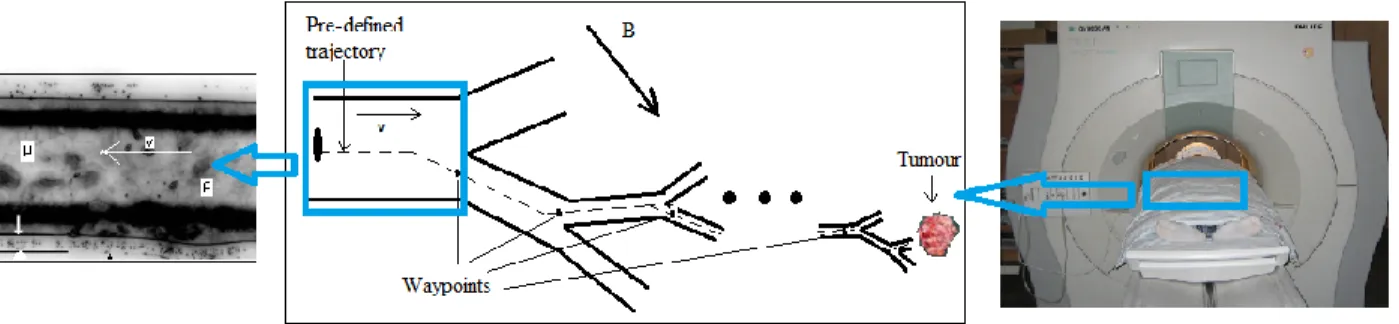
The microparticles, used as specialized drug carriers in our MR-Sub project, are supposed to be released from a catheter at a branch of human cardiovascular system where the catheter cannot access due to its size. Therefore, an appropriate control algorithm is required to navigate the microparticles after being released to travel along a series of waypoints and to pass through multiple bifurcations of blood vessels with MR gradients to finally reach the tumour position. Figure 2-1 shows a schematic diagram of this kind of intravascular navigation.
Figure 2- 1Schematic diagram of MR-Sub intravascular navigation
There are several constraints to the dedicated control algorithm.
1. It is demanded to become a real-time closed loop control, as feedbacks could be obtained from the MRI scanner in real-time.
2. The environment parameters such as the flow velocity or the blood pressure alter rapidly every time microparticles travel in different kinds of blood vessels, thus the controller needs to have good performance on robustness to resist external interferences.
3. Until now, clear and precisely-described mathematical models could hardly be found to model the blood fluid in human cardiovascular system. Complex non-linearity has been introduced. All kind of factors such the heartbeat, the vasomotion and the blood flow swirl increase vastly the uncertainty as well as the randomness of the whole human vascular system environment.
4. It would be more preferable if the controller has a very short responds time so as to save time for navigating the microparticles because sometimes microparticles travel at a really high velocity inside the blood vessel.
5. As a result of the high horizontal velocity of the blood flow, there is no method to define the microparticle entry zone to a certain bifurcation, i.e., the microparticle may access anywhere inside the parent branch of the bifurcation when injected. Hence, the real travelling trajectory of the microparticle could never be pre-calculated or previewed and each time the controller has to face to a new and also unique control problem.
6. The output of the controller would be programmed as MR sequences to generate gradients for steering the microparticles. However, the MR gradients seem not to be a perfect continuous output for control but have non-negligible rising time and falling time. It is also fairly important to take the sequence properties into consideration when designing the controller.
Here, we may now look further into the main obstacle of control, i.e., microparticles usually travel with the flow inside blood vessels at a very high velocity.
Figure 2-2 shows one typical bifurcation of human cardiovascular system on which analysis will be conducted.
In Figure 2-2, the parent branch of the bifurcation has a length of 15.0mm as well as a diameter of 2.3mm. The start point is placed in the up left section of the parent branch while the current waypoint is placed in the down side which indicated that microparticles will need to be navigated from the start point into the daughter branch B. The dynamic viscosity and the density of the blood flow inside the vessel are 0.0035Pa∙s and 1060kg/𝑚3 respectively. The flow, as well as the microparticles, goes from left to right and travels at an average horizontal velocity of 0.15m/s, as it is commonly assumed that microparticles travel with the flow inside blood vessels.
In this case, the ideal control solution should be capable of driving microparticles to travel at least 1.15mm in vertical direction before microparticles reach the junction or current waypoint. With the model described in Figure 2-2, it could be proved (in Chapter 3) that, in the vertical direction, the drag force follows the Stoles law thus the absolute value of maximum vertical velocity to which microparticles might possibly reach could be calculated as follows:
‖ ⃗⃗⃗ 𝑚 ‖ ‖ ‖
Equation 2.1
Hence, the minimum time to be consumed for one microparticle covering a distance of 1.15mm in vertical direction would be:
_ 𝑚 ‖ ⃗⃗⃗⃗ ‖ Equation 2.2
Combining Equation 2.1 and 2.2, and substituting the symbols with real clinic values, we could calculate that _ 𝑚 .
It should be noticed that this result is obtained under all ideal circumstances. In the deduction, the necessity of acceleration procedure in the vertical direction of the microparticle is ignored. Moreover, the magnetic steering force is assumed to be induced at maximum power all the way along the steering process on the microparticle, which is also hardly possible to be realised.
However, with an average horizontal velocity of 0.15m/s, the previewed average time for a microparticle to pass the parent branch of the bifurcation could be estimated as follows:
𝑚 ⁄ Equation 2.3
As we have _ 𝑚 here, therefore, it could be then concluded that basically it is impossible to navigate hundred percent of microparticles into the correct daughter branch as desired. The optimal control method could only concern about how to raise the percentage of the quantity of navigated microparticles over a total amount. This high velocity obstacle will be further discussed in details in chapter 5.3.1.
2.3 Methodology
Nowadays, the most popular control theories include the classical control, the modern control theory using state transition matrix, the fuzzy control theory, the predictive control theory, etc., and all of their combinations.
One common trait for the classical control theory such as the simple PID theory or the modern control theory is that both of them strongly rely on an accurately-described mathematical model for the analysis of the controlled object motion. Hence, while in the situations that contain multiple non-linear, time-varying parameters which is hardly possible to find a consistent mathematical model or is hardly possible to run the precise model with a computer, the classical control theory and the modern control theory may show their limitations.
In the case of MR-Sub project, the lack of a precise mathematical model that fits all the conditions of the motion of microparticles inside different kinds of blood vessels is a major obstacle for designing a classical PID controller or a modern controller as most of the environment parameters are non-linear and time-varying. Due to the instability of blood flow, all those parameters need to be re-collected each time the microparticles enter a new bifurcation and thus the control parameters require online re-adjustments. Also, considering the MR sequence features and the fast responds time requirements, a self-adaptive fuzzy control algorithm is then proposed.
The fuzzy control algorithm replaces the concept of precise values with the concept of fuzzy values [14]. For an arbitrary set A in a domain Y and an element x, unlike the classical set theory raised by Georg Cantor which has an absolute declaration of x A or x A, the fuzzy set theory utilizes a membership function to reflect the extents of elements belonging to the set. For example, , whose range is a closed interval [0, 1], reflects the extent of x belonging to A. When , it shows that x has a very high tendency to be included in A, while it shows that x has a low tendency to belong to A if . When Y is a finite set { 3 }, the Zadeh representation of fuzzy set A is given as follows [14]:
Equation 2.4
where is the membership of belongs to A.
The fuzzy control algorithm maps every input fuzzy set to an output fuzzy set according to multiple fuzzy rules. The creation of fuzzy rules imitates the human thought process which mostly depends on common experiences of human experts. For example, suppose that we have the input fuzzy set A = {raining heavily} in the domain Y = {weather conditions} and an output fuzzy set O = {umbrella} in the domain Z = {Belongings}, a fuzzy rule R_F could be created as equation 2.2 to control the human behaviour:
R_F : if A then O Equation 2.5
which means that if it is raining heavily then take an umbrella. Hence, in such weather systems, once the precise input weather value x has a high extent of belonging to A, i.e., , the fuzzy controller responses automatically with an output control command of taking un umbrella.
As illustrated above, the fuzzy control process could be concluded as follows: first the controller takes the precise values for the inputs, and then it does fuzzifications of the precise values with membership functions of the input fuzzy sets. After deciding the extents of belonging to the fuzzy sets, the controller picks a specific value from the output fuzzy sets as the output of the whole control system in accordance with the corresponding fuzzy rules.
Since this kind of control is based on the experiences of human operators, and since it uses membership functions instead of precise values for describing the inputs, it tends to have less dependence on mathematical models and thus has more tolerance of external noises or alterations of environment parameters. Moreover, the fast responding time of the fuzzy controller could also be promised as its control process is as simple as a process of table look-up and output. Therefore, for the intravascular navigation of our MR-Sub application, the fuzzy controller has the potential to be a possible solution.
In the MR-Sub application, our crucial consideration for applying the fuzzy control is that, microparticles that have distinctions in positions or velocities should be treated differently. As shown in Figure 2-3, the whole zone of a branch of blood vessel that microparticles may access to is divided into finite number of sections. Each section is represented as an input fuzzy set. The boundaries between sections need to be defined by calculations of membership functions.
Figure 2- 3 Schematic diagram of fuzzification process of inputs
Having obtained the feedbacked coordinates of the microparticles from the MRI scanner at the beginning of a tracking-propulsion time period, the fuzzy controller would first calculate the fuzzy representations for inputs, and then determine one or several input fuzzy sets which conform with the particular position and velocity of microparticles at that time by comparing their membership functions. After that, a fuzzy reasoning process would be carried out using fuzzy rules corresponding to the related fuzzy sets based on expert operators’ experiences. A unique controller output for the MR gradient is given afterwards which would then be transferred to MR sequences and be executed during this tracking-propulsion time period to steer microparticles until another tracking process begins.
The steering magnetic force for microparticles would be mainly applied to the vertical direction of the blood flow. And in the horizontal direction we assume that microparticles travel at the same velocity of blood flow and their motion could hardly be affected by magnetic forces.
A Matlab/C++ simulation platform for navigating a single microparticle and microparticle aggregations was set up to verify the fuzzy control algorithm for intravascular navigation. Fuzzy parameters are amended according to simulation and experiment results. The optimisation of fuzzy control will be discussed in the next chapters.
CHAPTER
3:
MODELING
3.1 MR sequence and magnetic force
The system considered to fulfill the intravascular navigation is an upgraded Siemens Avanto 1.5T clinical MRI machine.
Figure 3- 1 Overview of real-time pulse sequence for 3-D control environment [4, 15]
The software architecture of the standard MRI system consists of two major parts: the Applications Environment and the Image Environment, as shown in Figure 3-1 [4, 15]. The Application environment is mainly responsible for the generation of MR sequences for tracking or propulsion while the Image Environment reconstructs MR images using the k-space data acquired from the running tracking sequence. Figure 3-1 shows an overview of a standard 3-D real-time sequence with time multiplexed positioning and propulsion phases.
As shown in Figure 3-1, the Application Environment module starts a period circle by performing a 3-D tracking process. The Image Environment collects k-space data from the
tracking process triggered in the Application Environment module. With the k-space data, the Image Environment is able to calculate and finally obtain the current 3-D coordinates of the under-controlled microparticle. After that, the Image Environment module will send the coordinate information back to the main propulsion controller located inside the Application Environment Module. The controller makes decisions according to the given coordinates and generates propulsion gradients. After the execution of the propulsion gradients, the Application Environment starts another “Tracking-Propulsion” circle.
Nowadays, with the modern real-time MRI feedback capabilities, the Image Environment module reconstructs images at the same time when Application Environment is running sequences and it is able to feedback before the next tracking-propulsion process begins which then allows the presence of a closed loop control infrastructure [3, 4]. In this case, the minimal time to acquire the xyz-coordinates of current position of a certain microparticle is , and the paused running sequence is . Thus the time left for a controller to calculate and apply 3-D propulsion gradients is .
In the next several chapters of this thesis, a much simplified MR sequence generation model as shown in Figure 3-2 which combines the Application module and Image module will be used for the simulations as well as the experiments.
In Figure 3-2, there are some important factors related to the control process, i.e., t_track for the tracking unit of the Application module to take images and return the current coordinates of a microparticle; the maximum magnetic gradient ∇ B to be reached in the next propulsion period and the time t_maintain to maintain that maximum gradient; the rising time t_rise and the falling time t_fall allowing the gradient to go to its maximum in the next propulsion period and to drop back to 0 afterwards. The adjustment factor ∆t_maintain is used to add to the reference value
t_maintain to make it more flexible and accurate. The important point here is that with current
MRI system, the propulsion could not be executed while the tracking sequence is running at the same time. That is to say, the MRI propulsion unit has to maintain a zero output during the time when tracking and positioning are in progress (t_track). This kind of trapezoidal MR sequence will be repeated finite times to provide a steering force for microparticles to select a correct pathway to the tumour position.
Figure 3- 2 Simplified MR real-time propulsion pulse sequence diagram
Taking the magnetic gradient ∇B⃗⃗⃗⃗⃗ , the magnetic force which is induced by a MRI gradient coil and which is applied to a piece of ferromagnetic artefact inside the magnetic gradient environment could be expressed as
F⃗ mag Vf M⃗⃗⃗ ∇⃗⃗ B⃗⃗ Equation 3.1
where F⃗ mag is the magnetic force (N), Vf is the volume of the ferromagnetic entity (𝑚3), M⃗⃗⃗ is the magnetization of the material (A/m), ∇B⃗⃗⃗⃗⃗ is the induced magnetic gradient (T/m).
3.2 Blood fluid
As a start, for a single bifurcation of the blood vessel, a 2-D coordinate system depicted in Figure 3-3 is set up in our study of modelling for the blood flow.
First the blood is assumed to be a Newtonian fluid as the Newtonian model has been applied adequately so far in the common blood flow problems including the local dynamics of flow through vascular junctions [16] because of its simplicity and because of the lack of alternatives as well.
Figure 3- 3 Coordinate system for a single bifurcation
To further determine the fluid type along the x-axis, the Reynolds number must be specified. In the x-axis, we have:
Re_p Equation 3.2
where Re_p is the Reynolds number for the blood flow parallel to the x-axis, U is the average flow velocity in that direction (m/s), D is the diameter of the pipe (m), ν and represent the kinematic viscosity and the dynamic viscosity respectively, ρ is the flow density (kg/𝑚3). In the case of intravascular microparticle navigation, parameters are introduced to get a result of Re_p 104.5.
Since in the x-axis, the Reynolds number Re_p 2000, the fluid along could be treated as Laminar flow in which fluid elements move only in the main flow direction [16], as shown in Figure 3-3, i.e., in our simulation and experiments, the fluid component of the main flow along y-axis is not considered.
In the direction along y-axis, an approximate result of the Reynolds number is also calculated as follows so as to calculate the fluid drag force applied to microparticles when they are driven to veer inside the blood vessel:
Re_v
∇
Equation 3.3
where Re_v is the Reynolds number for the flow perpendicular to x-axis (or parallel to y-axis), Vy is the steering velocity of the particle (m/s), r is the radius of the microparticle (m). Here, in our case, the maximum Reynolds number in y-axis obtained is Re_v 0.1283 1. Hence, the simplified Stokes Law could be applied to calculate the fluid drag force for the direction perpendicular to x-axis which is:
_ ⃗ Equation 3.4
where _ is the fluid drag force in y-axis.
There is another important property for a fluid inside a tube which is called “No-Slip Boundary Condition”. It states that in fluid flow there could not be any “step” change in velocity at any point within the flow field. As a result, fluid in contact with thestationary boundary must have zero velocity. This is because if a step change occurs near the boundary, the velocity gradient needs to be infinite and thus the force required maintaining the velocity gradient has to be infinite as well which is absolutely not possible [16].
Bases on the conclusion that the blood fluid is within the type of Laminar flow, a Poiseuille flow model assumption is then raised to better embody the “No-Slip Boundary Condition”. Figure 3-4 shows the velocity profile in steady fully developed Poiseuille flow [16, 17].
In the Poiseuille flow model, as one of its properties, a numerical relationship could always be discovered between the local velocity in x-axis of a certain point inside the blood vessel and the average velocity which could be indicated as follows:
where is a local velocity at a certain point inside the blood vessel, ma and avg are the maximum velocity and average velocity of the flow in x-axis, stands for the distance from the certain point to the middle of the vessel, stands for the radius of the vessel.
Figure 3- 4 Velocity profile in steady fully developed Poiseuille flow
In the present simulation, if a microparticle a is already stuck into a boundary as it appears in Figure 3-4, we assume that the boundary is rigid thus the particle still has a tiny distance against the boundary which would be its diameter r and still has a small velocity along x-axis. In reality however, it tends to be possible that microparticles would be pushed fiercely by the magnetic force against a boundary and stop moving. Further discussion will be done in the next several chapters to propose a method to prevent this situation from happening.
3.3 Force analysis for microparticles
Since the gravity force and the buoyancy force are negligible comparing with the other forces applied, 2-D force decomposition on a single microparticle is depicted in Figure 3-5. As microparticles are always travelling at the same speed as the blood flow in x-axis, they keep a stationary state relative to the blood flow in horizontal direction. Thus the compression forces from the flow to the microparticle are not depicted in Figure 3-5.
Figure 3- 5 Decomposition of forces on a single microparticle under navigation
Taking the equations 3.1 and 3.4, in the major steering direction (y-axis), an equation to describe the motion of microparticles under navigation is established from the simple Newton’s Law:
_ _ ( ⃗⃗ ∇⃗⃗ )B⃗⃗ 𝑚 Equation 3.6
where 𝑚 represents the mass of the ferromagnetic microparticle while is the distance that the particle has travelled along the y-axis.
CHAPTER
4:
CONTROLLER
4.1 Fuzzy controller overview
To provide steering force along the y-axis (as plotted in Figure 3-3), a SIMO Mamdani fuzzy controller is designed based on the mathematical model proposed in Chapter 3.
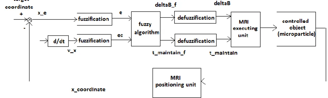
Figure 4-1 depicts the block diagram of closed-loop real time control applying the SIMO fuzzy controller.
Figure 4- 1 Closed-loop SIMO fuzzy control block diagram
For navigating a single microparticle, the single input of the whole control system would be the difference of the x-coordinate of the target microparticle and the x-coordinate of the next waypoint which is feedbacked by the MRI positioning unit by conducting a tracking sequence. Having obtained the velocity along x-axis of the particle from the derivative of the input, the controller determines the values of ∇ B and ∆t_maintain shown in Figure 3-2 according to the current position and velocity of the microparticle as the two critical elements of the MR sequence and outputs. The MRI propulsion unit would then execute the sequence in the following propulsion period to create a magnetic force in y-axis to steer the target microparticle and maintain it until the next tracking-propulsion period begins.
For navigating a microparticle aggregation, the only difference is that the input would be the difference of the x-coordinate of the gravity center of the aggregation and the x-coordinate of the next waypoint.
In the following sections, the fuzzification process of inputs for the fuzzy controller core and the defuzzification process of outputs will be discussed. Fuzzy rule sets will be given depending on operators’ experience.
4.2 Fuzzification of inputs and defuzzification of outputs
The fuzzy sets for both the inputs and the outputs of the controller core are defined as {Negative Big (NB), Negative Medium (NM), Negative Small (NS), Zero (O), Positive Small (PS), Positive Medium (PM), Positive Big (PB)}. The membership function definitions for the two inputs are given over a field of {-6, -5, -4, -3, -2, -1, 0, 1, 2, 3, 4, 5, 6} while those for the two outputs are defined over a field of {-7, -6, -5, -4, -3, -2, -1, 0, 1, 2, 3, 4, 5, 6, 7}.
4.2.1 Input of coordinate
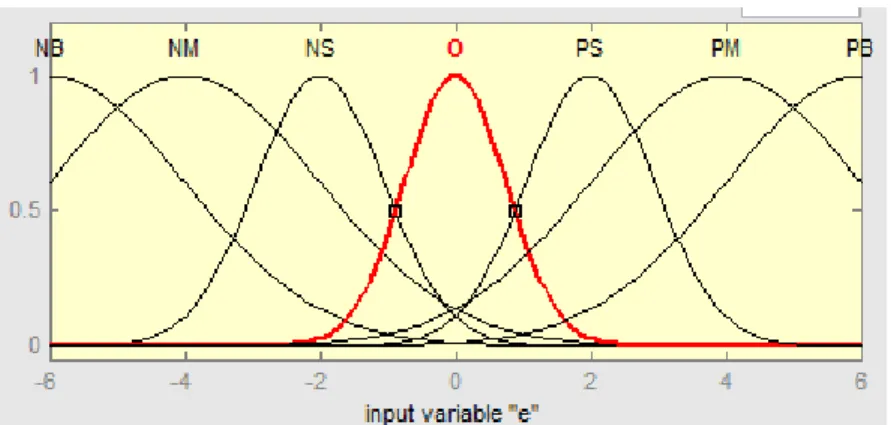
The membership functions selected for the coordinate input are normal distribution functions, as the normal distribution is the most common probability distributions in nature. Therefore, the membership functions represented with normal distributions tend to allow input errors over a wider range.
The membership functions for coordinate input are given as follows:
{ 3 Equation 4.1
where all the normal distribution parameters have been corrected through all simulations and experiments.
Figure 4-2 plots the coordinate input membership functions over a field of { }.
Figure 4- 2 Membership functions for coordinate input -E
Figure 4-2 indicates that when a coordinate input has been mapped from the real number field to the fuzzy field, it could have multiple corresponding input fuzzy sets. For example, the fuzzy controller would understand that an input of “+4” in the fuzzy field has a high possibility of belonging to the fuzzy set Positive Medium (PM), a fair possibility of belonging to the fuzzy set Positive Big (PB), a low possibility of belonging to the fuzzy set Positive Small (PS), and a scarce possibility of being included in any other fuzzy sets.
Table 4.1 lists the quantized membership functions of the coordinate input, preserving one significant figure after the decimal point.
Table 4. 1 Quantized membership functions of coordinate input -E
-6 -5 -4 -3 -2 -1 0 +1 +2 +3 +4 +5 +6 NB 1.0 0.8 0.4 0.1 NM 0.4 0.8 1.0 0.8 0.4 0.1 NS 0.3 1.0 0.3 O 0.2 1.0 0.2 PS 0.3 1.0 0.3 PM 0.1 0.4 0.8 1.0 0.8 0.4 PB 0.1 0.4 0.8 1.0
In our MR-Sub application, since it is crucial to decide whether the microparticles have passed the current waypoint or not (If it has already passed the current waypoint, although not significant, a new navigation loop needs to be started as soon as possible to save time for the second bifurcation navigation.), a high resolution and control sensibility are required. Therefore, the membership functions describing the concepts “O”, “PS”, “NS” are set to be acuter at the top than the other ones [11, 18].
4.2.2 Input of velocity
Ideally, the input of velocity needs to be first calculated from the derivative of the input of coordinate. However, since the tracking is a sampling process in discrete time, the velocity along x-axis of a target microparticle or the center of mass of an aggregation of microparticles is obtained using the formula below:
‖ ⃗⃗⃗ ‖ p ‖p p ‖
Equation 4.2
where ‖ ⃗⃗⃗ ‖ is the absolute value of the velocity along x-axis of the particle or the aggregation, is the real-time x-coordinate feedback, is the recorded x-coordinate for the penultimate tracking process, t_track is the time for tracking, are the rising time, maintaining time and falling time for the last sequence respectively.
For the same reason, the membership functions of the velocity input are using normal distribution functions defined below:
{ 3 Equation 4.3
where all the normal distribution parameters have been tested and corrected through all simulations and experiments.
Figure 4-3 plots the velocity input membership functions over a field of { }.
Figure 4- 3 Membership functions for velocity input -EC
Table 4.2 lists the quantized membership functions of the velocity input, preserving one significant figure after the decimal point.
Table 4. 2 Quantized membership functions of velocity input -EC
-6 -5 -4 -3 -2 -1 0 +1 +2 +3 +4 +5 +6 NB 1.0 0.2 NM 0.2 1.0 0.2 NS 0.4 1.0 0.4 O 0.2 0.6 1.0 0.6 0.2 PS 0.4 1.0 0.4 PM 0.2 1.0 0.2 PB 0.2 1.0
In this case, the membership functions corresponding to fuzzy sets “NB” and “PB” have acuter tops. This is because when microparticles have a high x-velocity, the difficulty of control is increased and a higher control sensibility is required.
4.2.3 Output of magnetic gradient
The magnetic gradient is one critical output for the fuzzy control core as it decides the maximum absolute value for depicted in Figure 3-2.
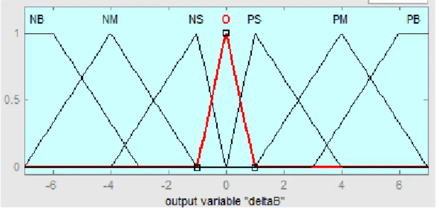
As there is no outputting error, triangular distribution functions are chosen for membership functions mainly because of the ease of calculation.
{ ( ) ( ) ( ) 3 ( ) ( ) ( ) ( ) Equation 4.4
Figure 4-4 plots the magnetic gradient output membership functions over a field of { }.
Figure 4- 4 Membership functions for magnetic gradient output -G
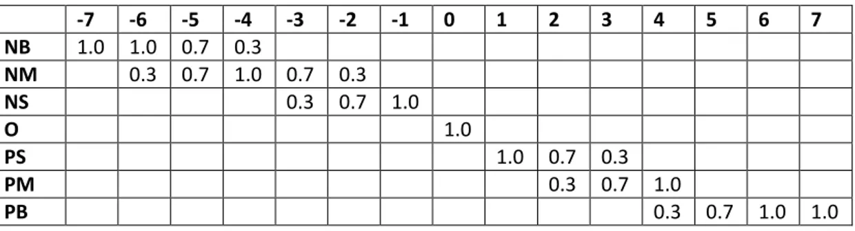
Table 4.3 lists the quantized membership functions of the magnetic gradient output, preserving one significant figure after the decimal point.
Table 4. 3 Quantized membership functions of magnetic gradient output -G -7 -6 -5 -4 -3 -2 -1 0 1 2 3 4 5 6 7 NB 1.0 1.0 0.7 0.3 NM 0.3 0.7 1.0 0.7 0.3 NS 0.3 0.7 1.0 O 1.0 PS 1.0 0.7 0.3 PM 0.3 0.7 1.0 PB 0.3 0.7 1.0 1.0
4.2.4 Output of maximum gradient maintaining time adjustment ∆t_maintain
The maximum gradient maintaining time adjustment output describes the factor t_maintain and ∆t_maintain depicted in Figure 3-2. This output is essential as the controller needs to discriminate the situations when the microparticles demand full power propulsion or when the microparticles are travelling at a low velocity thus more times for tracking could be gained.
The reason why the controller gives a direct output of ∆t_maintain instead of t_maintain is that the time factor could not be negative. If t_maintain is used for direct output, the whole negative part of the fuzzy controller would then be meaningless, resulting in a narrow self-regulation range.
The triangular distributed membership functions are given as follows:
{ ( ) ( ) ( ) 3 ( ) ( ) ( ) ( ) ( ) ( ) ( ) Equation 4.5
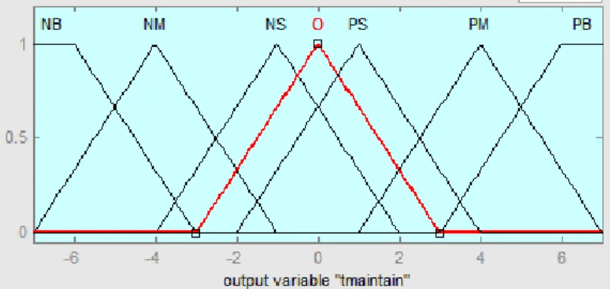
Figure 4-5 plots the maximum gradient maintaining time adjustment output membership functions over a field of { }.
Figure 4- 5 Membership functions for maximum gradient maintaining time adjustment -T
Table 4.4 lists the quantized membership functions of the maximum magnetic gradient maintaining time adjustment output, preserving one significant figure after the decimal point.
Table 4. 4 Quantized membership functions of maintaining time adjustment output -T
-7 -6 -5 -4 -3 -2 -1 0 1 2 3 4 5 6 7 NB 1.0 1.0 0.7 0.3 NM 0.3 0.7 1.0 0.7 0.3 NS 0.3 0.7 1.0 0.7 0.3 O 0.3 0.7 1.0 0.7 0.3 PS 0.3 0.7 1.0 0.7 0.3 PM 0.3 0.7 1.0 0.7 0.3 PB 0.3 0.7 1.0 1.0
4.3 Fuzzy rule sets
Normally, the fuzzy rule sets consist of a series of “IF A THEN B” condition judgements, where A usually is a combination of fuzzy input sets and B represents fuzzy output sets.
4.3.1 “IF...THEN...” fuzzy judgments
The “IF...THEN...” fuzzy judgements are determined mainly according to expert operators’ experience as well as simulation and experiment results.
In our application, the basic design philosophy is that microparticles with different positions or velocities should be treated separately.
The rule sets are designed in the format as follows:
{ Equation 4.6
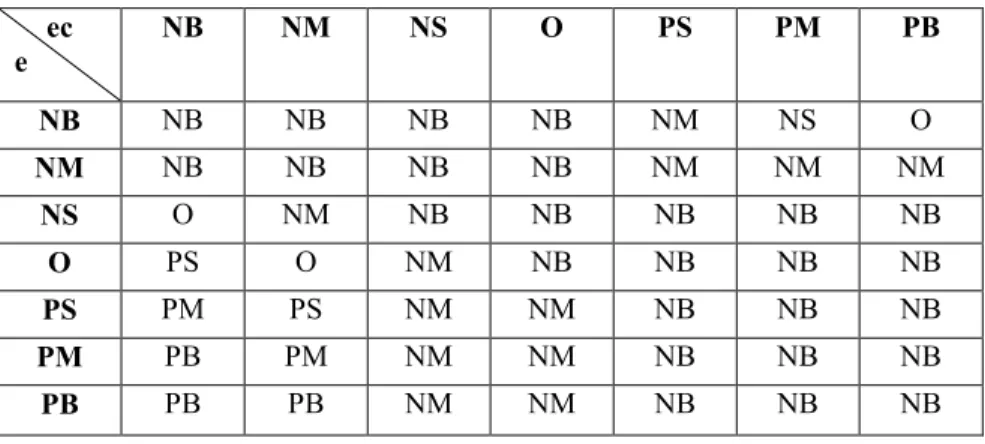
Since we do not have any coupling between the two outputs, the SIMO fuzzy control problem (MIMO for the control core) could then be divided into two Single-Input-Single-Output problems. Table 4.5 and Table 4.6 list the two rule sets R1 for magnetic gradient output and R2 for maximum gradient maintaining time adjustment output respectively.
Table 4. 5 Rule sets R1 for magnetic gradient output
ec e NB NM NS O PS PM PB NB O O O O NS NS NM NM PS PS O O O O NS NS PM PM PS PS O O NS O PB PM PM PM PM PS O PS PB PM PM PM PM PS O PM PB PB PM PM PS PS O PB PB PB PM PS PS O O
Table 4. 6 Rule sets R2 for maintaining time adjustment output ec e NB NM NS O PS PM PB NB NB NB NB NB NM NS O NM NB NB NB NB NM NM NM NS O NM NB NB NB NB NB O PS O NM NB NB NB NB PS PM PS NM NM NB NB NB PM PB PM NM NM NB NB NB PB PB PB NM NM NB NB NB
4.3.2 Quantized fuzzy outputs
For each output, we have 49 rules. Then the total fuzzy implication relation could be expressed as follows:
⋃ Equation 4.7
The quantized outputs are calculated using the formulas below (Take rule set R1 as an example): ⋃ ⋃ { } Equation 4.8 ⋃ { ⋂ } ⋃ { ⋂ } ⋃
In these formulas, the interaction “ ” simply uses the minimum weight of all the antecedents, the synthetic algorithm “ ” uses the max-min method and the implication “ ” also takes the minimum weight.
The defuzzification of fuzzy outputs uses the "centroid" method, i.e., to take the weighted arithmetic mean of its membership function as the output to the executing unit of the MRI system, e.g., for the output ▽B, the defuzzification applies
∑ ∑
Equation 4.9
where denotes the membership functions which are shown in Figure 4-4.
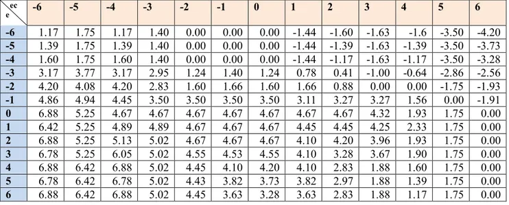
By programming with Matlab/Simulink Tool box, the quantized fuzzy control output tables are presented in Table 4.7 and Table 4.8 (See Annexe 1), preserving two significant figures after the decimal point. Linear transformations have been already operated to these tables to enlarge controllable area.
Table 4. 7 Quantized fuzzy output table for magnetic gradient
ec e -6 -5 -4 -3 -2 -1 0 1 2 3 4 5 6 -6 1.17 1.75 1.17 1.40 0.00 0.00 0.00 -1.44 -1.60 -1.63 -1.6 -3.50 -4.20 -5 1.39 1.75 1.39 1.40 0.00 0.00 0.00 -1.44 -1.39 -1.63 -1.39 -3.50 -3.73 -4 1.60 1.75 1.60 1.40 0.00 0.00 0.00 -1.44 -1.17 -1.63 -1.17 -3.50 -3.28 -3 3.17 3.77 3.17 2.95 1.24 1.40 1.24 0.78 0.41 -1.00 -0.64 -2.86 -2.56 -2 4.20 4.08 4.20 2.83 1.60 1.66 1.60 1.66 0.88 0.00 0.00 -1.75 -1.93 -1 4.86 4.94 4.45 3.50 3.50 3.50 3.50 3.11 3.27 3.27 1.56 0.00 -1.91 0 6.88 5.25 4.67 4.67 4.67 4.67 4.67 4.67 4.67 4.32 1.93 1.75 0.00 1 6.42 5.25 4.89 4.89 4.67 4.67 4.67 4.45 4.45 4.25 2.33 1.75 0.00 2 6.88 5.25 5.13 5.02 4.67 4.67 4.67 4.10 4.20 3.96 1.93 1.75 0.00 3 6.78 5.25 6.05 5.02 4.55 4.53 4.55 4.10 3.28 3.67 1.90 1.75 0.00 4 6.88 6.42 6.88 5.02 4.45 4.10 4.20 4.10 2.83 1.88 1.60 1.75 0.00 5 6.78 6.42 6.78 5.02 4.43 3.82 3.73 3.82 2.97 1.88 1.39 1.75 0.00 6 6.88 6.42 6.88 5.02 4.45 3.63 3.28 3.63 2.83 1.88 1.17 1.75 0.00
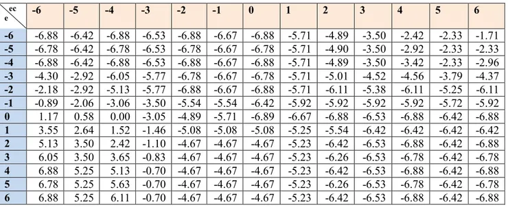
Table 4. 8 Quantized fuzzy output table for maximum gradient maintaining time adjustment ec e -6 -5 -4 -3 -2 -1 0 1 2 3 4 5 6 -6 -6.88 -6.42 -6.88 -6.53 -6.88 -6.67 -6.88 -5.71 -4.89 -3.50 -2.42 -2.33 -1.71 -5 -6.78 -6.42 -6.78 -6.53 -6.78 -6.67 -6.78 -5.71 -4.90 -3.50 -2.92 -2.33 -2.33 -4 -6.88 -6.42 -6.88 -6.53 -6.88 -6.67 -6.88 -5.71 -4.89 -3.50 -3.42 -2.33 -2.96 -3 -4.30 -2.92 -6.05 -5.77 -6.78 -6.67 -6.78 -5.71 -5.01 -4.52 -4.56 -3.79 -4.37 -2 -2.18 -2.92 -5.13 -5.77 -6.88 -6.67 -6.88 -5.71 -6.11 -5.38 -6.11 -5.25 -6.11 -1 -0.89 -2.06 -3.06 -3.50 -5.54 -5.54 -6.42 -5.92 -5.92 -5.92 -5.92 -5.72 -5.92 0 1.17 0.58 0.00 -3.05 -4.89 -5.71 -6.89 -6.67 -6.88 -6.53 -6.88 -6.42 -6.88 1 3.55 2.64 1.52 -1.46 -5.08 -5.08 -5.08 -5.25 -5.54 -6.42 -6.42 -6.42 -6.42 2 5.13 3.50 2.42 -1.10 -4.67 -4.67 -4.67 -5.23 -6.42 -6.53 -6.88 -6.42 -6.88 3 6.05 3.50 3.65 -0.83 -4.67 -4.67 -4.67 -5.23 -6.26 -6.53 -6.78 -6.42 -6.78 4 6.88 5.25 5.13 -0.70 -4.67 -4.67 -4.67 -5.23 -6.42 -6.53 -6.88 -6.42 -6.88 5 6.78 5.25 5.63 -0.70 -4.67 -4.67 -4.67 -5.23 -6.26 -6.53 -6.78 -6.42 -6.78 6 6.88 5.25 6.11 -0.70 -4.67 -4.67 -4.67 -5.23 -6.42 -6.53 -6.88 -6.42 -6.88
Figure 4-6 and Figure 4-7 plot the input-output surfaces of the fuzzy controller.
Figure 4- 6 Input-Output surface for the fuzzy implication (E×EC)->G
4.4 Controller design discussion
The assumption that blood follows a Poiseuille flow model is fairly important in the design of this kind of fuzzy controller. Since the MRI positioning unit is capable of feedbacking in real-time the x-coordinate as well as the y-coordinate of microparticles, a Multiple-Input-Multiple-Output (MIMO) fuzzy controller is firstly considered. However, as the Poiseuille flow model is introduced, a numerical relation could then be always discovered between y-coordinate and x-velocity of the same microparticles by using Equation 3.5. Hence, the SIMO fuzzy control algorithm is finally released with the purpose of decreasing its complexity. To design the fuzzy rule sets R, we should be aware that the velocity input EC not only describes the motion of microparticles, but also reports the position of the navigation target in y-axis.
In essence, since the current MRI system is only able to run a sequence of propulsion or a sequence of tracking at a time, the outputs of fuzzy controller for magnetic gradient G and maintaining time adjustment T reflect a weigh of balance in putting the priority on propulsion or on tracking. Figure 4-8 shows the design approach of the fuzzy controller rule sets.
High magnetic gradient output always brings long rising time and falling time. Hence, low magnetic gradient as well as short maintaining time could be expected to save time for more tracking chances when priority is put on tracking, while propulsion priority normally leads to high magnetic gradient outputs and long maximum gradient maintaining time.
Among the five typical intravascular zones A, B, C, D, E plotted in Figure 4-8, priority will be put on propulsion for B and C to perform maximum power propulsion because of the high x-velocity. Microparticles inside zone A are supposed to be monitored frequently for the reason that the magnetic gradient may need to be switched to maximum power at any time. Zone D or E has a priority on tracking as the control effect should be evaluated as soon as possible before preparing for the next bifurcation navigation and having self-adjustments.
The fuzzy control rule sets also have definitions of outputs when the x-coordinate of the controlled target becomes negative or when its x-velocity becomes positive (which means that microparticles are actually receding from the next waypoint in x direction). This is not only due to the completeness requirement of controller design, but also because it is supposed that a well-designed fuzzy controller may demand a self-adaptive capability in case that the microparticles have already passed the branch but in a wrong direction misled by some burst errors or environmental disturbances. Although it is not possible to drive microparticles to travel upstream inside the blood vessel with our current clinical MRI system, we leave the potential to do this kind of self-adaptive control targeted to increase the robustness of the controller.
As to the problem described in the section 3.2 that microparticles may sometimes be pushed fiercely against a vessel boundary by the induced magnetic force which could prevent them from moving towards the next waypoint, new fuzzy rules may be added. A possible solution to this problem is that to create new rules for the controller to apply a tiny magnetic gradient in the opposite direction, as long as zero x-velocity of the target is being observed for a period of time. However, since the boundary is assumed to be rigid in our simulations and our in-vitro experiments, this kind of problem has never been encountered and thus is not considered in the proposed fuzzy controller.
CHAPTER
5:
SIMULATIONS
5.1 Introduction
Using the mathematical model proposed by Equation 3.6, a computer-aided simulation platform is established to simulate the motion of microparticles under the navigation of the SIMO fuzzy controller inside blood vessels with Matlab/C++ hybrid programming.
Branch models of blood vessels with one single bifurcation and multiple bifurcations are both introduced to the simulation. To better verify the performance of the controller, navigation attempts on a single microparticle and on an aggregation of microparticles are also both made.
5.2 Software architecture
The program flow chart for simulation platform is shown in Figure 5-1.
Figure 5- 1 Program flow chart for simulation platform
The program is run with an infinite loop consisting of four sequence processes in the order of a real MR sequence until the navigated target reaches its destination.
Inside the four main processes, time is divided into tiny time slots by a certain time step to perform the differential operation according to Equation 3.6, as depicted in Figure 5-2.
Figure 5- 2 Process programming flow chart
Figure 5-3 shows the deducing process of coordinates as well as velocities in a single time slot operation.
Figure 5- 3 Deducing process of coordinates and velocities in a single time slot operation
![Figure 3- 1 Overview of real-time pulse sequence for 3-D control environment [4, 15]](https://thumb-eu.123doks.com/thumbv2/123doknet/2343396.34340/30.918.111.804.276.721/figure-overview-real-time-pulse-sequence-control-environment.webp)