Two-dimensional numerical analysis of the Poiseuille–Bénard flow in a rectangular channel heated from below

HAL Id: hal-01946109

https://hal.archives-ouvertes.fr/hal-01946109

Submitted on 5 Dec 2018

HAL is a multi-disciplinary open access

archive for the deposit and dissemination of

sci-entific research documents, whether they are

pub-lished or not. The documents may come from

teaching and research institutions in France or

abroad, or from public or private research centers.

L’archive ouverte pluridisciplinaire HAL, est

destinée au dépôt et à la diffusion de documents

scientifiques de niveau recherche, publiés ou non,

émanant des établissements d’enseignement et de

recherche français ou étrangers, des laboratoires

publics ou privés.

Two-dimensional numerical analysis of the

Poiseuille–Bénard flow in a rectangular channel heated

from below

Xavier Nicolas, Abdelkader Mojtabi, Jean Karl Platten

To cite this version:

Xavier Nicolas, Abdelkader Mojtabi, Jean Karl Platten. Two-dimensional numerical analysis of the

Poiseuille–Bénard flow in a rectangular channel heated from below. Physics of Fluids, American

Institute of Physics, 1997, 9 (2), pp.337-348. �10.1063/1.869235�. �hal-01946109�

OATAO is an open access repository that collects the work of Toulouse

researchers and makes it freely available over the web where possible

This is an author’s version published in:

http://oatao.univ-toulouse.fr/20671

To cite this version:

Nicolas, Xavier and Mojtabi, Abdelkader and Platten, J. K.

Two-dimensional numerical analysis of the Poiseuille–Bénard

flow in a rectangular channel heated from below. (1997)

Physics of Fluids, 9 (2). 337-348. ISSN 1070-6631

Official URL:

https://doi.org/10.1063/1.869235

Open Archive Toulouse Archive Ouverte

Any correspondence concerning this service should be sent

Two-dimensional numerical analysis of the Poiseuille–Be´nard flow

in a rectangular channel heated from below

X.NicolasandA.Mojtabi

Institut de Me´canique des Fluides, UMR CNRS/INP-UPS 5502, Universite´ Paul Sabatier, UFR MIG, 118 route de Narbonne, 31062 Toulouse Cedex, France

J.K.Platten

Laboratoire de Chimie Ge´ne´rale, Faculte´ de Me´decine, Universite´ de Mons-Hainaut, 7000 Mons, Belgium

The Poiseuille–B´enard flow ~PBF! is studied by a two-dimensional numerical simulation for a Prandtl number equal to 6.4 ~that of water at 23 °C! and for a wide range of Rayleigh ~Ra! and Reynolds ~Re! numbers: Ra<6000 and Re<3. The two observed flow configurations are ~1! thermally stratified Poiseuille flow and ~2! thermoconvective transversal rolls superimposed to the basic Poiseuille flow. The time evolution of the velocity components, the spatial development of the transversal rolls, their frequency, wavelength and velocity, the Nusselt number, together with the stability map in the Ra–Re plane, are studied in detail. Whenever possible, quantitative comparisons are made with published results: most of the experimental data, based on laser-Doppler anemometry ~LDA!, are recovered with amazing accuracy; a good agreement with results of convective stability deduced from a weakly nonlinear Ginzburg–Landau theory is also obtained.

I. INTRODUCTION

The Poiseuille–Be´nard flow ~PBF! is a mixed convec-tion flow in a horizontal rectangular channel heated from below. This problem has been widely studied, particularly because of its practical or technological interest. During this first half century, research on this subject attempted to ex-plain certain meteorological phenomena like the cloudy band alignment under the action of the wind.1,2 More recently, applications have been concerned with technological pro-cesses like the cooling of electronic components3,4 or the production of thin films in CVD~chemical vapor deposition! reactors;5–10 these works have mainly focused on the heat transfer enhancement related to thermoconvective structures in the flow. Because of the richness of its dynamical behav-ior, the PBF has also given rise to fundamental studies on the stability of the different thermoconvective patterns that are liable to arise. The present paper is in keeping with these studies.

The PBF is the result of the superimposition of two con-vective sources:~1! a horizontal pressure gradient giving rise to a forced flow, characterized by its Reynolds number Re, and~2! a vertical temperature gradient ~characterized by its Rayleigh number Ra! the source of thermoconvective struc-tures.

Results of linear hydrodynamic stability theory11–13have shown that the thermally stratified Poiseuille flow~the ‘‘ba-sic flow’’! keeps stable as long as Ra does not exceed a certain critical value Ra*_{~cf. Fig. 1!. Beyond this value, the}

basic flow becomes unstable and two kinds of thermocon-vective structures, called ‘‘transversal rolls’’ and ‘‘longitudi-nal rolls,’’ may appear. The transversal rolls, R_' ~respec-tively longitudinal rolls, Ri! have their axes perpendicular

~respectively parallel! to the direction of the mean flow. While the longitudinal rolls are stationary structures, the transversal rolls are carried away out of the channel by the

average flow; they can be considered like a quasi-two-dimensional ~2-D! structure, while in the longitudinal rolls the three velocity components are excited. In the case of ducts of infinite lateral extension~the transversal aspect ratio

B5l/h5`, where l and h are, respectively, the channel

width and height!, the longitudinal rolls are shown to appear first @Fig. 1~a!#, since the critical Rayleigh number for the longitudinal rolls, Ra_i*_{51708, is always smaller than Ra'}* ~the critical Rayleigh number for the transversal rolls!. For finite rectangular ducts @Fig. 1~b!#, the lateral confine-ment has two effects: first, it tends to stabilize the basic flow @when B decreases, Ra*5min(Ra_'*,Ra_i*) grows; Ra*.1708#; second, the vertical lateral boundaries promote

the appearance of the transversal rolls at Re smaller than a critical value Re*; when Re.Re*, the main flow favors the longitudinal rolls. Note that Ra_'*depends not only on Re and

B, but also on the Prandtl number Pr: when Pr increases,

Ra_'*increases. Since Ra_i* is not modified by Pr, Re* dimin-ishes when Pr increases. Thus, for Pr'0.7 ~air! Re*'7 ~see

Refs. 14 and 15! and for Pr'6.4 ~water! Re*'0.3 ~see Refs.

14 and 16!. The very small value of Re*explains why, for a long time, only a few works have been devoted to the trans-versal roll behavior or to the transition R_'– Ri, comparing

with the literature dealing with the longitudinal rolls. It is important to note that the stability diagram in Fig. 1 is the result of a linear analysis, only valid near the critical Rayleigh number Ra*. When investigating the nonlinear be-havior of the PBF, the structure of the flow becomes much more complex. Experimental works by Ouazzani et al.14,16,17 or by Chiu and Rosenberger,9 recent 3-D numerical simulations15,18 and studies based on a weakly nonlinear Ginzburg–Landau model19,20have shown that the transition

R_'– Riis not as sharp as it is represented in Fig. 1. Near the

triple transition point K @Fig. 1~b!#, the transversal and lon-gitudinal rolls compete and periodic or intermittent patterns

can arise.17 Furthermore, in some conditions, transversal or longitudinal rolls, can be observed for the same set of the dimensionless parameters, according to the initial conditions. Considering first only transversal rolls, Mu¨ller et al.21 have applied the concept of convective instability in the PBF and defined a new critical Rayleigh number for the transver-sal rolls, Ra_'conv.Ra_'* ~Fig. 2!. When Ra_'*,Ra,Ra_'conv_{, the} flow is convectively unstable: a local perturbation, appearing at time t₀ at x5x₀ ~cf. Fig. 2!, will be allowed to increase with time in a moving frame of reference, but it will be

damped, at each point of the duct, for a long enough time.22 In our case and in the domain of convective instabilities, it will be necessary to sustain a perturbation by a forcing~or a white noise! to create a global pattern, i.e., transversal rolls. When Ra.Ra_'conv, the flow is absolutely unstable: any local perturbation~Fig. 2! will grow at all points of the duct until it asymptotically reaches saturation and the establishment of the transversal rolls.

In their study, Mu¨ller et al.21 carry out a 2-D numerical simulation of the PBF, for the transversal roll configuration and for Pr51, in order to validate the Ginzburg–Landau am-plitude equation. Recently, Ouazzani et al.23 have adapted the results of the preceding study to the case of water ~Pr 56.4! to compare with experiments based on LDA investi-gations; they show that the transition between the thermally stratified Poiseuille flow and the transversal rolls favorably compares with Ra_'conv, but not with Ra_'*: the transition closely corresponds to the convective instability curve, not to the neutral one.

In the present paper results are reported on the transver-sal roll behavior obtained by a 2-D direct numerical simula-tion. A part of these results refer to the experiments of Ouaz-zani et al.14,16in order to quantitatively compare experiments and theory. Therefore, the Prandtl number of the fluid is equal to 6.4; the flow is systematically studied for Reynolds and Rayleigh numbers such that Re,3 and Ra,6000. Thus, all the presented results cover a wide range of dimensionless parameters, from the linear to the nonlinear domain. When-ever possible, comparisons with the studies of Mu¨ller

et al.21,23,24are also given. The specific problems linked with the numerical simulation of convective patterns and open flows on finite computational domains are presented; in par-ticular, the influence of the boundary conditions at the outlet of the channel and that of the periodic boundary conditions will be dealt with.

After having presented the methodology used to com-pute the PBF, the results are discussed in five distinct parts. First, quantitative comparisons with Ouazzani’s experi-ments, are made concerning the evolution of the vertical ve-locity component W with Ra and Re; most of the experimen-tal measurements of this velocity component, obtained by LDA in Ref. 16, are numerically reproduced with amazing accuracy. Simultaneously, the horizontal velocity compo-nent, U, and the average Nusselt number, Nu, on the top and bottom plates for the fully established transversal roll flow, are recorded and discussed.

Then, for numerous values of Ra and Re, the space de-velopment of the transversal rolls is visualized by means of a stationary intensity envelope of W. The characteristic growth length, l_e, of the transversal rolls is deduced from these en-velopes and is shown to be in very good agreement with the result obtained by the Ginzburg–Landau theory.23

In the next part, the stability map of the 2-D numerical PBF is presented. It shows the transition between the Poi-seuille flow and the transversal rolls ~the only two configu-rations that can be observed by 2-D simulation! in the Ra–Re plane. Ra_'*, Ra_'convand the different convective pat-terns encountered in Ouazzani’s experiments are projected

FIG. 1. Schematic presentation and stability diagram~result of the linear stability theory! of different configurations encountered in the PBF; ~a! PBF between two infinite horizontal plates; ~b! PBF in a channel with infinite longitudinal aspect ratio and finite lateral aspect ratio.

FIG. 2. Critical Rayleigh numbers for the transversal roll configuration ac-cording to the linear and convective stability criteria; schematic presentation of the space and time evolution of a small perturbation in the cases of absolutely stable flows and convectively and absolutely unstable flows.

on this map. The good agreement with the criterion of con-vective instability can be verified.

Then, the space and time average Nusselt number,^Nu&, is favorably compared with a theoretical formula given by Mu¨ller24 and valid on a weakly nonlinear domain ~Ra ,2500!. The numerical values of ^Nu& are obtained from two different configurations of the computational domain, using two different kinds of inlet and outlet boundary condi-tions. By means of the Nusselt number, the transition from the transversal rolls to the Poiseuille flow is shown to satisfy the criterion of convective stability when open boundary conditions ~OBC! are used at the outlet of the domain, whereas the criterion of linear stability is verified when pe-riodic boundary conditions are imposed.

Finally, we focus on the transversal roll frequency f , wavelength l, and velocity. To our knowledge, the present work is one of the few studies dealing with the wavelength evolution in the PBF, for a wide range of the parameters in a nonlinear domain. On the other hand, it is well known4,12,14–16,18,25that the transversal roll velocity, Vr, can be from 10% to 50% higher than the average velocity, U°, of the flow; the ratio Vr/U° is also shown to decrease lin-early with Ra, but to be independent of Re. In this paper, we present several results for Vr/U° at Pr56.4 and we show that it is possible to precisely reproduce the results obtained by the Ginzburg–Landau model.24

II. METHODOLOGY

The numerical code used to simulate the 2-D PBF solves the three conservation equations~mass, momentum, and en-ergy! on a rectangular domain of length L and height h, uniformly heated from below~at temperature Th! and cooled

from above~at temperature Tc!; the no slip boundary

condi-tions are applied to the velocity on the top and bottom plates. A Newtonian and incompressible fluid is considered and the Boussinesq approximation is assumed to be valid. Thus, the dimensionless governing equations in primitive variables ~velocity vector V, pressure P, temperature T! can be written as “ –V50, ~1! ]V ]t 1~V–“!V52“P1 1 ReDV1 Ra Re2 PrTk, ~2! ]T ]t1V–“T5 1 Re PrDT, ~3!

where the characteristic length, velocity, pressure, and tem-perature for scaling are h, U°,r~U°!2, and (Th2Tc),

respec-tively. Therefore, the Reynolds number Re5U°h/n, the Ray-leigh number Ra5gb(T_h2T_c)h3/na, and the Prandtl number Pr5n/a. Here r is the mass per unit volume,n the kinematic viscosity, g the gravitational acceleration, b the thermal expansion coefficient, and a the thermal diffusivity.26In addition, k is the upward vertical unit vector. The numerical code used to treat the incompressibility constraint and the velocity–pressure coupling between the mass and momentum equations, is based on the augmented lagrangian method27,28 and the use of a Uzawa-type

algorithm.29 ~For more details about the method and the nu-merical aspects see Ref. 30.! The equations are discretized by a finite volume method on a staggered grid. The convec-tive terms are discretized by a second-order centered differ-encing and the diffusive terms are approximated by second-order centered derivatives. The time scheme is Gear’s second-order backward implicit scheme; the time step Dt 50.0005 is used for all the unsteady computations. The lin-ear systems are solved with a preconditioned conjugate gra-dient method.30

All the computations have been realized on the same geometrical configuration ~noted config-1! but, in a few cases, two other configurations~config-2 and config-3! have been studied.

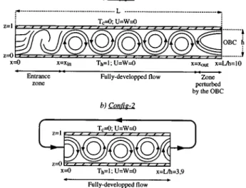
Config-1: @Fig. 3~a!# this is a ten aspect ratio duct (A

5L/h510). ~However, in some cases clearly mentioned, this aspect ratio will be equal to 20.! The inlet boundary conditions are a Poiseuille profile for velocity and a linear profile for temperature. At the outlet boundary, several OBC have been tested and compared;30an Orlanski31-type bound-ary condition has been chosen allowing the smallest ampli-tude perturbation at the outlet. The boundary conditions are summarized in Table I.

All the computations with config-1 have been achieved with the following space steps in the axial and spanwise directions: (Dx;Dz)5~0.1; 0.05!. This configuration allows

FIG. 3. Schematic presentation of the transversal roll development and of the boundary conditions for the two main computational configurations used;~a! config-1: thermally stratified Poiseuille flow at the inlet and open boundary condition at the outlet;~b! config-2: periodic boundary conditions.

TABLE I. Boundary conditions used to compute the PBF with config-1. Inlet~x50! Bottom~z50! Top~z51! Outlet (x5L/h)

U(0,z,t)56(z2z2_{) U(x,0,t)50 U(x,1,t)50} ]U

]t1U 0]U ]x50 W(0,z,t)50 W(x,0,t)50 W(x,1,t)50 ]W ]t 1U 0]W ]x50 T(0,z,t)512z T(x,0,t)51 T(z,1,t)50 ]T ]t1U 0]T ]x50

us to observe the space amplification of the perturbation until nonlinear saturation occurs; when thermoconvection devel-ops in the PBF, three zones can be distinguished@Fig. 3~a!#: ~1! for 0<x<xin, the entrance zone in which the perturba-tion is growing; then, after its saturaperturba-tion,~2! for xin<x<xout, a fully established periodic flow of transversal rolls; and~3! near the outlet, for xout<x<L/h, a small zone where the rolls are slightly distorted by the OBC. In most of our simulations, the length of this third zone is smaller than h but can be higher in a few runs due to its divergence at the critical point.30Note that, for a fixed Rayleigh number, the length of the entrance zone increases when the Reynolds number in-creases; sometimes, transversal rolls do not even appear in the domain of computation at high Reynolds numbers, espe-cially for small Rayleigh numbers. Numerically, this con-figuration allows us to compute the characteristic growth length, l_e, of the transversal rolls, and consequently, to de-termine Ra_'conv, defined by the divergence of l_e.21

Config-2: to be able to analyze the fully established

ther-moconvective flow, especially for small Ra, periodic bound-ary conditions have been implemented30@Fig. 3~b!#. Further-more, as at each time step, a transversal roll that leaves the computational domain is simultaneously sent to the inlet, config-2 allows us to determine Ra_'*; indeed, when being in the convectively unstable flow phase, the perturbations at the outlet are continuously reinjected at the entrance: a kind of forcing is maintained at the inlet of config-2.

The transversal roll wavelength, l, is imposed by the aspect ratio A of the domain. Computations with config-1 having shown that l'1.95, we take here A53.9; thus, four transversal rolls may develop in config-2. Furthermore, (Dx;Dz)5~0.078; 0.05!.

Config-3: taking advantage of the fact that, in config-2,

the flow is periodic from the entrance to the outlet of the computational domain, it is possible to make the flow sta-tionary with a frame of reference moving at the same veloc-ity as the transversal rolls. Thus, config-3 is the same as config-2 except that, using a very simple change of variable in Eqs.~1!–~3! the rolls are made stationary. Note that it has then been possible to take Dt50.01, instead of Dt50.0005, without losing accuracy.

To be complete, it can be added that, whatever the con-figuration, two initial conditions have been used: either an isothermal Poiseuille flow~at temperature T_c!, or an already thermoconvective flow of transversal rolls; no hysteresis phenomenon has been observed with these conditions.

III. RESULTS AND DISCUSSION

All the results presented in the five following parts were obtained in the case of config-1, unless otherwise stated.

A. Comparison with experiments — preliminary observations

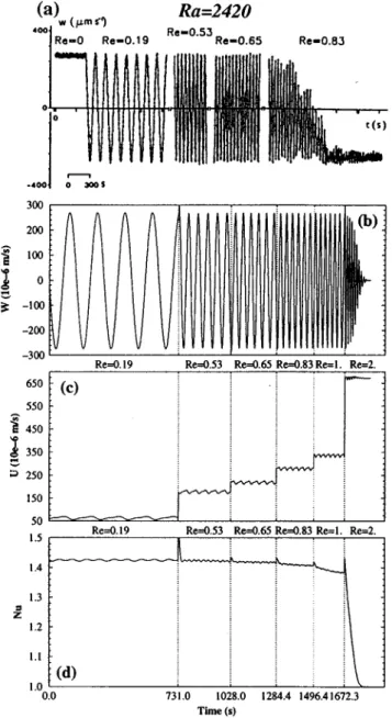
As a first result of the numerical simulation of the PBF, four particular flows are presented in Figs. 4, 5, 6 and 7. Figure 4 represents the time evolution of the experimental ~part a! and computed ~part b! vertical velocity component

W, of the computed horizontal velocity component U~part c!

and of the space average Nusselt number Nu on the top and

bottom plates ~part d!, at Re50.21 for an increasing Ray-leigh number. Figures 5, 6, and 7 represent the same quanti-ties for an increasing Re, respectively, for Ra52420, 2024, and 1804.

The computed velocity components, U and W, are re-corded at midheight of the channel ~z50.5!, at x57.5. The numerical signals obtained by recording the dimensionless W at each time step are presented dimensionally ~inmm/s! in view of a comparison with the equivalent experimental data obtained by LDA in Refs. 14 and 16. These experimental recordings are realized at midheight, at 6.5 cm from the en-trance of the channel, i.e., at (x,z)5~15.7, 0.5!. For conve-nience, they are reproduced in Figs. 4~a!, 5~a!, 6~a!, and 7~a! of this paper: these are, respectively, the Figs. 6 and 7 of Ref.

FIG. 4. Time evolution in the transversal roll phase, of the vertical [W(t)] and horizontal [U(t)] velocity components and of the space average Nusselt number@Nu(t)# for Re50.21, Ra51804, 2074, 2490, 2896, and 3460, and for Pr56.4; ~a! W(t) at (x,z)5~15.7, 0.5! from the experiments of Ouazzani

et al.;14,16_{~b!,~c!,~d!, respectively, W(t), U(t), and Nu(t) at (x,z)5~7.5,}

16, Figs. 5–18 of Ref. 14, and Fig. 10 of Ref. 16. The time evolution of U and Nu are only given for the numerical simulations since these quantities were not measured in the experimental available papers. Nu is defined as follows:

Nu~t!5 1 x22x1

E

FS

D

S

D

G

The average over the length of the duct is taken between

x₁54 and x₂58.5 in order to avoid the inlet and outlet zones

in the evaluation of the mean. This is usually sufficient, ex-cept for extremely small Rayleigh numbers.

In Figs. 4~a! and 4~b!, the sinusoidal behavior of W around a zero mean value characterizes traveling transversal

rolls. W_'max~the maximum vertical velocity component of the transversal rolls at midheight! increases with Ra and its square ~W_'max!2 is a linear function of Ra. The two signals, experimental and numerical, agree with each other, both in amplitude ~except at Ra51804! and in frequency f . At Re 50.21, f keeps constant whatever the Rayleigh number. It is approximately equal to 6.531023 s21 in Fig. 4~a! and

FIG. 5. The same as Fig. 4 for Ra52420 and Re50.19, 0.53, 0.65, and 0.83 ~plus Re51 and Re52 for the numerical simulation!; ~a! for the experiments,14,16_{transition to longitudinal rolls at Re50.83; ~b!,~c!,~d! for}

the 2-D numerical simulations, transition to the Poiseuille flow at Re52.

FIG. 6. The same as Fig. 4. for Ra52024 and Re50.15, 0.27, 0.42, 0.46, and 0.5 ~plus Re50.6 for the numerical simulation!; ~a! for the experiment,14transition to ‘‘intermittent pattern’’ at Re50.5; ~b!,~c!,~d! for the 2-D numerical simulation, persistence of the Poiseuille flow until Re 50.6.

7.1531023 s21 in Fig. 4~b!, that is to say a difference of 10%.

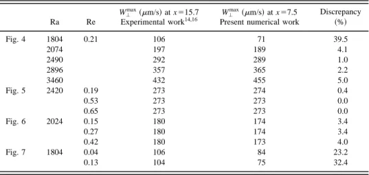
Concerning the amplitude, Table II gives W_'max for the experimental and numerical signals of Figs. 4, 5, 6, and 7. The maximum discrepancy between the two sets is less than 5%, except at the smallest Rayleigh number, Ra51804, where it can reach as much as 40%. This can partially be attributed to the difficulty of determining precisely the value

of the Rayleigh number in the experiments ~as already dis-cussed in Ref. 23!. Subsequently, as W_'maxis proportional to ~Ra/Ra_'conv_21!1/2_{, the relative error on W}

'maxincreases when

Ra tends to Ra_'conv. On the other hand, a part of the error can also be attributed to the position of the ‘‘measuring probe:’’

x515.7 in the experiments and x57.5 for the numerical

simulations. At Ra51804, at x515.7, the flow is fully devel-oped, whereas, at x57.5, we could still be in the entrance zone of the PBF, where the amplitude of W has not yet reached its maximum.

In Fig. 4~c!, the signal of U becomes bichromatic, show-ing the fundamental frequency f ~the same as for W! and the first harmonic 2 f . Their amplitudes increase with Ra. The harmonic 2 f has already been observed in the classical Rayleigh–Be´nard convection.32,33 A detailed analysis of all our numerical results shows that the amplitudes of the two modes are independent of the Reynolds number, at least in the fully developed zone@this is, however, not clearly visible in Figs. 5~c!, 6~c!, and 7~c!#. In all cases, the mean value of

U corresponds exactly to the maximum Poiseuille velocity.

Figure 4~d! shows the increase of the Nusselt number with Ra. The weak oscillations in the signal are due to the finite arbitrary width of the interval [x₁,x₂] in the computa-tion of Nu @cf. Eq. ~4!#, which do not necessarily contain a finite number of rolls. Consequently, we will note ^Nu& the time average Nusselt number over these oscillations:

^

&

t₂2t₁

E

Nu~t!dt, ~5!

where the time interval (t22t1) excludes the small initial transient phase when increasing the Rayleigh number.

In each of the Figs. 5, 6, and 7, the Rayleigh number is constant. If the Reynolds number is small enough ~for the values listed in Table II!, stabilized transversal roll flows are observed: W_'max~and ^Nu& in a lesser extent! keeps constant with Re ~cf. Table II!. In addition, the roll frequency in-creases linearly with Re ~shown in detail later!. In Fig. 5~a!, when Re increases, the flow undergoes experimentally a transition to longitudinal rolls (Ra.Ra_i*), characterized by a nonzero and constant vertical velocity component, at Ra 52420 and Re50.83; in the 2-D numerical simulation, the transition is to the Poiseuille flow, at Re52, characterized by

W50 and a constant U signal together with a Nusselt

num-ber equal to 1 @Figs. 5~b!–5~d!#. In Fig. 6, at a lower Ray-leigh number ~Ra52024!, the scenario remains the same, except for the so-called ‘‘intermittent pattern’’17 in the ex-perimental signal at Re50.5. In Fig. 7, for a still lower Ra ~Ra51804!, a transition to the Poiseuille flow is observed in the two cases since now Ra,Ra_i*; it occurs between Re 50.18 and Re50.25 in the experiments, and between Re 50.25 and Re50.5 in the numerical simulations ~a more precise determination yields Re50.36!. When the Reynolds number is reduced to the previous value Re50.13, transver-sal rolls with the same amplitude and the same frequency are restored.

As already mentioned before, an aspect ratio L/h510 computational domain is unsufficient to get fully established flows at the lowest Ra ~Ra51804 in Table II!. So, in the

FIG. 7. The same as Fig. 4 for Ra51804 and Re50.04, 0.13, 0.18, and 0.25 ~plus Re50.5 for the numerical simulation!; ~a! for the experiment,14,16

tran-sition to the Poiseuille flow at Re50.25; ~b!,~c!,~d! for the 2-D numerical simulation, transition to the Poiseuille flow at Re50.5.

subsequent paragraphs and figures, for Ra51804 and 1836,

L/h520 is always used and results in better agreement with

the experimental values of Table II.

B. Space development of the transversal rolls

As was already stated in the Introduction, the observed critical Rayleigh number compares with Ra_'conv and not with Ra_'*. In this paragraph, we want to numerically recover, for Pr56.4, previous results obtained experimentally and theo-retically concerning Ra_'conv; eventually, we also want to show that the numerical tool allows us to give results at high Rayleigh numbers, where a Ginzburg–Landau-type approach certainly fails to produce accurate results. Therefore, in Figs. 8 and 9, at different Ra and Re, we present numerous sta-tionary envelopes of the maximum vertical velocity compo-nent along the axis of the channel. More precisely, the plots of the figures give W_maxas a function of x, where

Wmax~x!5 max

tP@t₁,t₂# ~ max

zP@0,1#

W~x,z,t!!, ~6!

with t2.t1 and t1.tt, where ttis the time marking the end

of the transient flow phase.

As an example, let us focus on the graph drawn at Ra 51836 for which the computational domain has been ex-tended to L/h520 in order to avoid the effect of the OBC, clearly important at small Ra and Re. The saturation ampli-tude W_s, defined by

Ws5 max xP@x_in,x_out#

Wmax~x!, ~7!

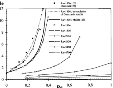
is equal to 102 mm/s. The characteristic growth length l_e is defined by W_max(l_e)5W_s/2. For each Reynolds number, l_e has been determined from the plots of Fig. 8, and is given in Fig. 10. Its divergence at Re'0.44 is clearly seen to coincide with the result of the amplitude equation23and to agree fairly well with the experiments ~dashed line!. The results at Ra 51804 and 2024 are also reported; of course, the divergence of l_e is found earlier~Re'0.36! at Ra51804 and later ~Re

'0.8! at Ra'2024. As a matter of fact, the procedure can be repeated for all the Rayleigh numbers presented in Fig. 8 and the divergence of le appears at higher Reynolds numbers

when Ra increases ~not shown in Fig. 10!. The Poiseuille

FIG. 8. For fixed Ra and several Re, stationary envelopes representing the space evolution of the maximum vertical velocity component along the axis of the channel, from the inlet to the outlet of config-1 domain; for Ra51804 and Ra51836, A5L/h520; for Ra52024, 2420, 3460, and 4700, A510. TABLE II. Comparison of the maximum vertical velocity component during the transversal roll phase, as a

function of Ra and Re, obtained experimentally by Ouazzani et al.14,16_{and numerically in the present work.}

Ra Re

W_'max_{~mm/s! at x515.7}

Experimental work14,16

W_'max_{~mm/s! at x57.5}

Present numerical work

Discrepancy ~%! Fig. 4 1804 0.21 106 71 39.5 2074 197 189 4.1 2490 292 289 1.0 2896 357 365 2.2 3460 432 455 5.0 Fig. 5 2420 0.19 273 274 0.4 0.53 273 273 0.0 0.65 273 273 0.0 Fig. 6 2024 0.15 180 174 3.4 0.27 180 174 3.4 0.42 180 173 4.0 Fig. 7 1804 0.04 106 84 23.2 0.13 104 75 32.4

flow is reached when Wmax(x)50 for all xP[0, L/h]; it is only shown for ~Ra, Re!5~1804, 0.5!, ~2024, 0.8!, and ~2420, 1.5! in Fig. 8, and for ~Re, Ra!5~0.5, 1875! and ~1, 2200! in Fig. 9.

In Fig. 11, the saturation amplitude of the vertical veloc-ity component, Ws, is shown to be independent of the

Rey-nolds number ~as it should be!, and is compared with the experiments of Ouazzani et al.14,16 The maximum discrep-ancy between the results of the two studies is at most 14

mm/s.

C. Stability diagram in (Ra–Re) plane

Figure 12 presents the stability diagram in the Ra–Re plane. The results of the linear12and of the convective21,23,24 stability theory, together with the experimental results of Ouazzani et al.14,16 are superimposed to the results of the present numerical work. The theoretical results apply to 2-D flows, whereas the experimental results are 3-D; conse-quently, the experiments allow more flow configurations and transitions.

Numerically, the nature of each point of the diagram, Poiseuille flow, or transversal rolls, is determined by follow-ing the evolution of a given transversal roll flow as initial conditions and updating Re and/or Ra. In some cases, we have verified that the choice of the initial conditions do not lead to hysteresis effects: the same transversal roll flow is computed starting with a conductive solution of the PBF and adding a small sinusoidal perturbation on W equal to 5% of the final amplitude of the rolls. In practice, very long CPU times are needed to compute the points near the transition

FIG. 9. For fixed Re and several Ra, stationary envelopes representing the space evolution of the maximum vertical velocity component along the axis of the channel, from the inlet to the outlet of config-1 domain; for Re50.21, 0.5, and 1, A5L/h510; for Re50.31, A520.

FIG. 10. Characteristic growth length over which the vertical velocity en-velope of the transversal rolls, Wmax(x), increases from the inlet to half its

value of saturation~Ws/2!, as a function of Re; at Ra51836, comparison

with Ouazzani’s experiment23_{and with a result obtained from the amplitude}

curve. Consequently, only 19 points have been computed to determine its position. Furthermore, to save computational time, all the computations, even for the smallest Rayleigh numbers, have been realized with config-1 for L/h510. However, a few times, L/h520 has been used in order to

assess the presence of the transversal rolls; for example, in Fig. 9, at Re50.31 and Ra51780, i.e. close to Ra_'conv, the instability seems to develop only after x510. Nevertheless, this remark is a function of the criterion used to determine the nature of the flow; in this study, it is considered that the transversal rolls disappear for the benefit of the Poiseuille flow when the following criterion is verified:

H

^

&

~8! Figure 12 shows that the numerical results coincide quite well with the results of the amplitude equation; therefore, the 2-D numerical simulations of the PBF with config-1 satisfies the convective stability criterion, not the linear one.

Experimentally, the stability diagram of the 3-D flow is much more complex. Ouazzani et al.14,16have identified five regions ~cf. Fig. 12!: for the small Rayleigh numbers ~zone I!, the Poiseuille flow keeps stable; for the bigger Rayleigh numbers the flow is thermoconvective: transversal rolls are always observed in II and longitudinal rolls in III; between these two zones, in IV, there are either transversal or longi-tudinal rolls, depending on the initial conditions; and, in the small zone V, the flow structure shows an intermittent char-acter for which the vertical velocity W oscillates around a nonzero mean value.16,17 Except for the smallest Reynolds

FIG. 11. Saturation amplitude of the vertical velocity component as a func-tion of Re, for the experiments of Ouazzani et al.14,16_{and for the present}

numerical work.

FIG. 12. Stability diagram of the different configurations encountered in the PBF with Pr56.4. The numerical results of the present work are obtained with config-1; other already published results are superimposed to the numerical solution.

numbers ~,Re*'0.3!, it is difficult to compare the

experi-mental stability diagram with the others: a 3-D numerical simulation would be necessary. Nevertheless, two 3-D nu-merical studies of the PBF can be pointed out: in Ref. 15, a zone IV is observed for a flow in a transversal aspect ratio 2 duct and for Pr50.7 ~even though this result seems to be linked with a numerical artefact: the choice of Dt!; in Ref. 18, with B5l/h54.1 and Pr5530 ~silicon oil!, Schro¨der and Bu¨hler show flow configurations where transversal and lon-gitudinal rolls superimpose; these solutions could be favor-ably compared with certain experimental signals obtained in region V by Ouazzani et al.14,17

D. Nusselt number

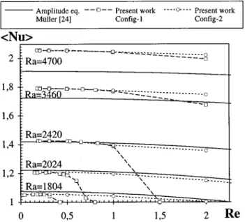
In Fig. 13, the space and time average Nusselt number ^Nu& is plotted as a function of Re for several values of Ra. The results of the numerical simulations, computed with config-1 and config-2, are compared with those obtained by Mu¨ller24and valid for a 2-D flow. From the amplitude equa-tion, Mu¨ller proposes the following formula to compute the horizontally average Nusselt number:

^

&

g

Ra2Ra_'*

Ra , ~9!

where, for Pr56.4,g50,699, i.e. 1/g51.4306 ~see Ref. 23!. On the other hand, Schlu¨ter et al.34give a formula valid on a linear domain for pure free convection and an infinite roll pattern between two horizontal plates:

^

&

Therefore, Mu¨ller’s formula ~9! is nothing else but the Schlu¨ter et al. formula ~10! in which 1708, is replaced by Ra_'*; thus,^Nu& in ~9! is a function of Re through Ra_'*and it is valid only for small Rayleigh numbers.

For the numerical computations with config-1 at Ra 51804, the Nusselt number is averaged from x1510 to

x2518 @cf. ~4!# because A520; in the other cases, A510 and the average is taken, as said before, from x154 to x258.5. For config-2, A53.9 and ^Nu& is averaged from x150.2 to

x253.7.

In the three different studies, the Nusselt number de-creases with Re. It tends to ^Nu&51, corresponding to the conductive Poiseuille flow. With config-1, this limit is reached when crossing the Ra_'convcurve, as it can be seen at Ra51804, 2024, and 2420. Obviously, ^Nu& obtained with config-1 and config-2 coincide very well whatever Ra, for small values of Re, i.e., for the cases where, in config-1, the transversal roll amplitude has reached its stationary value between x₁and x₂.

For config-2, ^Nu& decreases slightly with Re, until the value ^Nu&51 is reached when crossing the neutral critical curve Ra_'*. It has been computed earlier12that Ra_'*5 1804 at

Re52.27 and Ra_'* _{5 2024 at Re54.12. We find here that} ^Nu& drops to 1 at Ra51804 when Re'2.05 instead of 2.27 ~see the lower curve of Fig. 13!, and at Ra52024 when Re '4.2 instead of 4.12 ~not shown in Fig. 13!. The Nusselt number computed with Eq.~9! is in agreement with the nu-merically found values, at least at small Rayleigh numbers ~Ra<2420!. At higher Ra, Eq. ~9! cannot remain a good approximation.

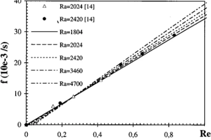
E. Transversal roll frequency, wavelength, and velocity

In Fig. 14, the transversal roll frequency f , computed with config-1, is plotted as a function of Re, for several Ray-leigh numbers. The frequency has been determined from the same type of signals as those presented in Figs. 4–7. For a fixed Rayleigh number, f is a linear function of Re. It has been verified that f does not vary with x, as long as x,xout. The numerical results are in good agreement with the experi-mental results of Ouazzani.14The fact that all the curves do not pass through the origin is attributed to the outlet OBC, a fact already observed and discussed in Ref. 18. With the use of periodic boundary conditions~config-2!, all the curves do pass through the origin. In contradistinction with Ref. 18 ~a study realized at a totally different Prandtl number Pr5530!, in which the authors found that f decreases when Ra in-creases whatever Re, we find in our simulations that this is only the case for Re,0.26; beyond, f increases slightly when Ra increases. This is due to the small mismatches of the wavelength in the two studies, conducted at very differ-ent Prandtl numbers.

The dimensionless wavelength,l, is plotted in Fig. 15. Here,l is computed averaging from the signals of U, W, and

FIG. 13. Space and time average Nusselt number as a function of Re and Ra; comparison of the numerical solutions obtained on config-1 and config-2 with the linear stability result obtained by Mu¨ller.24

T recorded for x₁<x<x₂, at eight different time steps for

t>t_t. From a single signal, when A510, Dx50.1, and

x₂2x₁54.5, l is approximately evaluated within 60.05.

But, by multiplying the number of signals ~both for U, W, and T at eight different times, i.e. 24 signals!, the error on l for each point of Fig. 15 is estimated to be less than 0.015 ~the error bars are drawn only for a few points!. So, in spite of an inaccuracy linked to the mesh size, l is shown to weakly decrease when Re and Ra increases ~except for the smallest Reynolds numbers Re<0.3!. This is in good quali-tative agreement with the result of the 2-D numerical simu-lation by Mu¨ller et al.21at Pr51, and with those of Schro¨der and Bu¨hler,18 who found the same tendency for l, even at Pr5530.

Figure 16 presents Vr/U°5l/t5@h2/~nRe!#f l as a function of Ra ~wheretis the dimensionless time period,l the dimensionless wavelength plotted in Fig. 15, but f is the frequency in s21plotted in Fig. 14!. As already said in the Introduction, the four plotted curves, corresponding to Ouaz-zani’s experiment,14,16 Mu¨ller’s 2-D theory,24 and to the present numerical results obtained with config-1 and config-3, decrease linearly with Ra and are independent of Re. The three 2-D studies give nearly the same curves, and

the linear stability result obtained by Luijkx12 in the case of infinite lateral extension ducts~Vr/U°51.29 interpolated for Pr56.4! is exactly reproduced by the amplitude equation theory and by the present simulations with config-3. Ouaz-zani’s 3-D result is also in good agreement with the linear stability theory,12where we estimate Vr/U°'1.5 at the criti-cal point for B5l/h53.6. Therefore, the difference between

Vr/U°51.29 and 1.5 is clearly due to the lateral confinement

of the fluid. The slope of the only available experimental curve has never been theoretically verified yet; a 3-D nu-merical simulation would be necessary.

For config-1, the curve of Fig. 16 is the result of the linear interpolation of Vr/U° computed from f andl; since

f increases with Ra~when Re>0.26!, the decrease of Vr/U°

is due to the faster decrease of l. The Re independence of

Vr/U° is determined within 60.03. The line equation is Vr/U°51.25420.9531025Ra.

Mu¨ller’s curve and that of the simulation with config-3 merge into one single straight line in the validity domain of the Ginzburg–Landau equation: for Ra,2500, Vr/U° 51.30821.3231025Ra. The curve with config-2~not drawn in the graph! is parallel and at 0.02 units below the curve of config-3. With the periodic boundary conditions, since l is constant, Vr/U° is more precisely determined than when l varies; the Re independence is once more verified, within 60.01 for config-2 and within 60.002 for config-3. Further-more, Vr/U° is not modified when the longitudinal aspect ratio A of these two configurations varies between 3.5 and 4.5: the roll frequency adjusts itself to the imposed wave-length so that the roll velocity remains the same. Finally, let us note that Hasnaoui et al.4have found a result very close to our finding for the roll velocity, also using periodic boundary conditions similar to config-2; their line equation, for Pr57, is Vr/U°'1.284–0.9031025Ra.

IV. CONCLUSION

In this study, numerous results characterizing the PBF, in a wide range of the dimensionless parameters Ra and Re,

FIG. 14. Transversal roll frequency, computed on config-1, as a function of Re and Ra and for Pr56.4; comparison with Ouazzani’s experiment14 at Ra52024 and 2420.

FIG. 16. Ratio of the transversal roll velocity, Vr, to the average velocity of the flow, U°, as a function of Ra and for Pr56.4; comparison of the numeri-cal solutions obtained on config-1 and config-3 with the experimental results of Ouazzani et al.14,16and with Mu¨ller’s theoretical result24 ~the limit of validity of this theory, Ra'2500, is indicated by a vertical line!. All the curves are independent of Re.

FIG. 15. Transversal roll dimensionless wavelength ~with error bars drawn for a few points!, computed on config-1, as a function of Re and Ra and for Pr56.4.

have been presented in detail; each time possible, they are validated thanks to quantitative comparisons with the already published experimental and theoretical works.

For the transversal roll configuration, the time evolution of the vertical velocity and the frequency have been shown to be in a very good agreement with the experiments of Ouazzani et al.,14,16 as soon as Ra.2000. The theoretical results of Mu¨ller et al.,21,23,24based on the Ginzburg–Landau amplitude equation and valid for Ra,2500, are also well reproduced: particularly, the results concerning the absolute instability-convective instability transition between the trans-versal rolls and the Poiseuille flow, the characteristic growth length l_e, the variation of the velocity Vr/U° with Ra, and the variation of the Nusselt number with Re. However, a 3-D numerical simulation seems to be necessary in view of an explanation of the experimental slope concerning Vr/U°, and, obviously, concerning the reproduction of the stability map and the numerous varieties of flow patterns experimen-tally observed~longitudinal rolls, intermittent patterns,...!.

Finally, it has been shown that the simulations with a computational configuration with OBC at the outlet~config-1 type! give the convective stability curve Ra_'conv, whereas a config-2 type configuration ~with periodic boundary condi-tions! simulates the linear stability curve Ra_'*.

ACKNOWLEDGMENTS

This work was supported by CNRS/CGRI-FNRS ~Grants EB/EUR-94/No. 41 and EB/EUR-95/No. 123!. The numerical simulations were performed on the IBM-SP2 com-puter of the CNUSC ~South University National Center of Computation!. The authors would like to thank the staff of the CNUSC for his availability concerning the technical sup-port and the training.

1_{H. Be´nard and D. Avsec, ‘‘Travaux re´cents sur les tourbillons cellulaires}

et les tourbillons en bandes; applications a` l’astrophysique et a` la me´te´o-rologie,’’ J. Phys. Rad. 9, 468~1938!.

2_{D. Brunt, ‘‘Experimental cloud formation,’’ Compendium of Meteorology}

~American Meteorological Society, Boston, 1951!, pp. 1255–1262.

3_{M. E. Braaten and S. V. Patankar, ‘‘Analysis of laminar mixed convection}

in shrouded arrays of heated rectangular blocks,’’ Int. J. Heat Mass Trans-fer 28, 1699~1985!.

4_{M. Hasnaoui, E. Bilgen, P. Vasseur, and L. Robillard, ‘‘Mixed convective}

heat transfer in a horizontal channel heated periodically from below,’’ Num. Heat Transfer, Part A. 20, 297~1991!.

5

G. Evans and R. Greif, ‘‘A study of traveling wave instabilities in a hori-zontal channel flow with applications to chemical vapor deposition,’’ Int. J. Heat Mass Transfer 32, 895~1989!.

6_{G. Evans and R. Greif, ‘‘Unsteady three-dimensional mixed convection in}

a heated horizontal channel with applications to chemical vapor deposi-tion,’’ Int. J. Heat Mass Transfer 34, 2039~1991!.

7_{G. Evans and R. Greif, ‘‘Thermally unstable convection with applications}

to chemical vapor deposition channel reactors,’’ Int. J. Heat Mass Transfer

36, 2769~1993!.

8

H. K. Moffat and K. F. Jensen, ‘‘Complex flow phenomena in MOCVD reactors—1. Horizontal reactors,’’ J. Cryst. Growth 77, 108~1986!.

9_{K. C. Chiu and F. Rosenberger, ‘‘Mixed convection between horizontal}

plates—1. Entrance effects,’’ Int. J. Heat Mass Transfer 30, 1645~1987!.

10

K. C. Chiu, J. Ouazzani, and F. Rosenberger, ‘‘Mixed convection between horizontal plates—2. Fully developed flow,’’ Int. J. Heat Mass Transfer

30, 1655~1987!.

11_{J. M. Luijkx, J. K. Platten, and J. C. Legros, ‘‘On the existence of}

ther-moconvective rolls, transverse to a superimposed mean Poiseuille flow,’’ Int. J. Heat Mass Transfer 24, 803~1981!.

12

J. M. Luijkx, ‘‘Influence de la pre´sence de parois late´rales sur l’apparition de la convection libre, force´e et mixte,’’ Ph.D. thesis, University of Mons-Hainaut, Belgium, 1983.

13_{J. K. Platten and J. C. Legros, Convection in Liquids ~Springer-Verlag,}

New York 1984!, Chaps. 6 and 8.

14

M. T. Ouazzani, ‘‘Transferts thermiques et me´canique des e´coulements de convection mixte,’’ Ph.D. thesis, University of Mons-Hainaut, Belgium, 1991.

15

S. S. Chen and A. S. Lavine, ‘‘Laminar, buoyancy induced flow structures in a bottom heated, aspect ratio 2 duct with throughflow,’’ Int. J. Heat Mass Transfer 39, 1~1996!.

16

M. T. Ouazzani, J. K. Platten, and A. Mojtabi, ‘‘Etude expe´rimentale de la convection mixte entre deux plans horizontaux a` tempe´ratures diffe´rentes—2,’’ Int. J. Heat Mass Transfer 33, 1417~1990!.

17_{M. T. Ouazzani, J. K. Platten, and A. Mojtabi, ‘‘Intermittent patterns in}

mixed convection,’’ Appl. Sci. Res. 51, 677~1993!.

18

E. Schro¨der and K. Bu¨hler, ‘‘Three-dimensional convection in rectangular domains with horizontal throughflow,’’ Int. J. Heat Mass Transfer 38, 1249~1995!.

19

H. R. Brand, R. J. Deissler, and G. Ahlers, ‘‘Simple model for the Be´nard instability with horizontal flow near threshold,’’ Phys. Rev. A 43, 4262 ~1991!.

20_{H. W. Mu¨ller, M. Tveitereid, and S. Trainoff, ‘‘Rayleigh–Be´nard problem}

with imposed weak through-flow: Two coupled Ginzburg–Landau equa-tions,’’ Phys. Rev. E 48, 263~1993!.

21_{H. W. Mu¨ller, M. Lu¨cke, and M. Kamps, ‘‘Convective patterns in}

hori-zontal flow,’’ Europhys. Lett. 10, 451~1989!.

22

R. J. Deissler, ‘‘Spacially growing waves, intermittency and convective chaos in an open flow system,’’ Physica D 25, 233~1987!.

23_{M. T. Ouazzani, J. K. Platten, H. W. Mu¨ller, and M. Lu¨cke, ‘‘Etude de la}

convection mixte entre deux plans horizontaux a` des tempe´ratures diffe´r-entes —3,’’ Int. J. Heat Mass Transfer 38, 875~1995!.

24_{H. W. Mu¨ller, ‘‘Thermische Konvection in horizontaler Scherstro¨mung,’’}

Ph.D. thesis, University of Saarlandes in Sarrebruck, Germany, 1990.

25_{M. T. Ouazzani, J. P. Caltagirone, G. Meyer, and A. Mojtabi, ‘‘Etude}

nume´rique et expe´rimentale de la convection mixte entre deux plans hori-zontaux a` tempe´ratures diffe´rentes,’’ Int. J. Heat Mass Transfer 32, 261 ~1989!.

26

Below are given the numerical values corresponding to the experimental conditions of Refs. 14, 16, 17, 23 and used for comparisons in the present paper. Geometrical characteristics of the channel: length in the x direction

L5115 mm, width in the y direction l515.05 mm, height in the z

direc-tion h54.15 mm, longitudinal aspect ratio A5L/h527.7, lateral aspect ratio B5l/h53.63. Physical characteristics of water at T523 °C: thermal diffusivity a50.14531026 m2_{/s, thermal expansion coefficient} b5237.6231026_K21_{, kinematic viscosityn50.93310}26_m2_/s. 27_{M. Fortin and R. Glowinski, Me´thodes de Lagrangien Augmente´,}

Appli-cations a´ la Re´solution Nume´rique de Proble`mes ausc Limites, Collection

Me´thodes Mathe´matique de l’Informatique—9, Dunod editeur ~Bordas, Paris, 1982!.

28_{R. Glowinski, Numerical Methods for Non-linear Variational Problems,}

Springer Series in Computational Physics~Springer-Verlag, New York, 1984!.

29_{K. J. Arrow, L. Hurwicz, and H. Uzawa, Studies in Nonlinear}

Program-ming~Stanford University Press, Stanford, CA, 1958!.

30_{X. Nicolas, P. Traore, A. Mojtabi, and J. P. Caltagirone, ‘‘Augmented}

Lagrangian method and open boundary conditions in the 2D simulation of the Poiseuille–Be´nard channel flow,’’ Int. J. Numerical Methods Fluids ~in press!.

31_{I. Orlanski, ‘‘A simple boundary condition for unbounded hyperbolic}

flows,’’ J. Comput. Phys. 21, 251~1976!.

32

P. Berge´, ‘‘Rayleigh–Be´nard instability: Experimental findings obtained by light scattering and other optical methods,’’ in Fluctuation, Instabilities

and Phase Transition, edited by T. Riste~NATO Advanced Study

Insti-tutes, Plenum Press, New York, 1975!, Vol. B11, pp. 323–352.

33_{C. Normand, Y. Pomeau, and M. G. Velarde, ‘‘Convective instability: A}

physicists approach,’’ Rev. Mod. Phys. 49, 581~1977!.

34_{A. Schlu¨ter, D. Lortz, and F. Busse, ‘‘On the stability of steady finite}