XCS Algorithms for a Linear Combination of Discounted and Undiscounted Reward Markovian Decision Processes

(1)

UNIVERSITÉ DE MONTRÉAL

XCS ALGORITHMS FOR A LINEAR COMBINATION OF DISCOUNTED AND UNDISCOUNTED REWARD

MARKOVIAN DECISION PROCESSES

MARYAM MOGHIMI

DÉPARTEMENT DE MATHÉMATIQUES ET DE GÉNIE INDUSTRIEL ÉCOLE POLYTECHNIQUE DE MONTRÉAL

MÉMOIRE PRÉSENTÉ EN VUE DE L’OBTENTION DU DIPLÔME DE MAÎTRISE ÈS SCIENCES APPLIQUÉES

(GÉNIE INDUSTRIEL) AOÛT 2018

(2)

UNIVERSITÉ DE MONTRÉAL

ÉCOLE POLYTECHNIQUE DE MONTRÉAL

Ce mémoire intitulé :

XCS ALGORITHMS FOR A LINEAR COMBINATION OF DISCOUNTED AND UNDISCOUNTED REWARD

MARKOVIAN DECISION PROCESSES

présenté par : MOGHIMI Maryam

en vue de l’obtention du diplôme de : Maîtrise ès sciences appliquées a été dûment accepté par le jury d’examen constitué de :

M. ADJENGUE Luc, Ph. D., président

M. BASSETTO Samuel, Doctorat, membre et directeur de recherche M. FRAYERT Jean-Marc, Ph. D., membre et codirecteur de recherche M. PARTOVI NIA Vahid, Doctorat, membre

(3)

DEDICATION

(4)

ACKNOWLEDGEMENTS

I would like to express my sincere gratitude to my supervisor Prof. Samuel Bassetto and my co-supervisor Prof. Jean-Marc Frayret for their support, patience, motivation and help to complete this project successfully.

I also would like to express my sincere thanks to my thesis committee: Professor Vahid Partovi nia and Professor Luc Adjengue for kindly evaluating my thesis.

Finally, I wish to thank my parents, my brothers, and my friends at CIMAR LAB for their support and their kindness.

(5)

RÉSUMÉ

Plusieurs études ont montré que combiner certains prédicteurs ensemble peut améliorer la justesse de la prédiction dans certains domaines comme la psychologie, les statistiques ou les sciences du management. Toutefois, aucune de ces études n'ont testé la combinaison de techniques d'apprentissage par renforcement. Notre étude vise à développer un algorithme basé sur deux algorithmes qui sont des formes approximatives d'apprentissage par renforcement répétés dans XCS. Cet algorithme, MIXCS, est une combinaison des techniques de Q-learning et de R-learning pour calculer la combinaison linéaire du payoff résultant des actions de l'agent, et aussi la correspondance entre la prédiction au niveau du système et la valeur réelle des actions de l'agent. MIXCS fait une prévision du payoff espéré pour chacune des actions disponibles pour l'agent. Nous avons testé MIXCS dans deux environnements à deux dimensions, Environment1 et Environment2, qui reproduisent les actions possibles dans un marché financier (acheter, vendre, ne rien faire) pour évaluer les performances d'un agent qui veut obtenir un profit espéré. Nous avons calculé le payoff optimal moyen dans nos deux environnements et avons comparé avec les résultats obtenus par MIXCS.

Nous avons obtenu deux résultats. En premier, les résultats de MIXCS sont semblables au payoff optimal moyen pour Environments1, mais pas pour Environment2. Deuxièmement, l'agent obtient le payoff optimal moyen quand il prend l'action "vendre" dans les deux environnements.

(6)

ABSTRACT

Many studies have shown that combining individual predictors improved the accuracy of predictions in different domains such as psychology, statistics and management sciences. However, these studies have not tested the combination of reinforcement learning techniques. This study aims to develop an algorithm based on two iterative approximate forms of reinforcement learning algorithm in XCS. This algorithm, named MIXCS, is a combination of Q-learning and R-learning techniques to compute the linear combination payoff and the correspondence between the system prediction and the action value. As such, MIXCS predicts the payoff to be expected for each possible action.

We test MIXCS in two two-dimensional grids called Environment1 and Environment2, which represent financial markets actions of buying, selling and holding to evaluate the performance of an agent as a trader to gain the desired profit. We calculate the optimum average payoff to predict the value of the next movement in both Environment1 and Environment2 and compare the results with those obtained with MIXCS.

The results show that the performance of MIXCS is close to optimum average reward in Environment1, but not in Environment2. Also, the agent reaches the maximum reward by taking selling actions in both Environments.

(7)

LIST OF TABLES

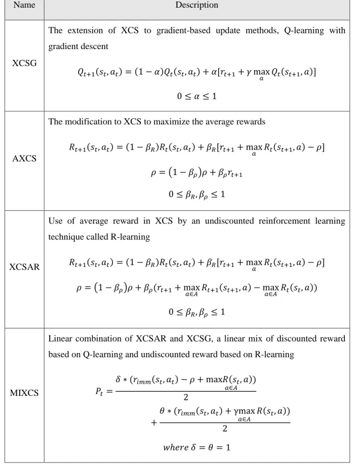
Table 3-1 : The summary of learning methods ... 35

Table 4-1 : Macro classifiers from the experiments ... 39

Table 4-2 : Numerosity for each possible action ... 39

(11)

LIST OF FIGURES

Figure 1-1: Combination of Q-learning and R-learning ... 3

Figure 2-1 : The possible actions in each state for agent ∗ ... 7

Figure 2-2 : Block diagram of reinforcement learning problem ... 10

Figure 2-3 : The learning classifier systems and environment ... 17

Figure 3-1: Detailed block diagram of XCS ... 23

Figure 3-2 : Block diagram of a committee machine based on ensemble averaging ... 30

Figure 3-3 : Environment1 ... 36

Figure 3-4 : Environment2 ... 36

Figure 4-1: Performance of applying MIXCS to Environment1 ... 40

Figure 4-2: Average reward of applying MIXCS to Environment1. ... 41

Figure 4-3: Population size in macro classifier for applying MIXCS to Environment1. ... 41

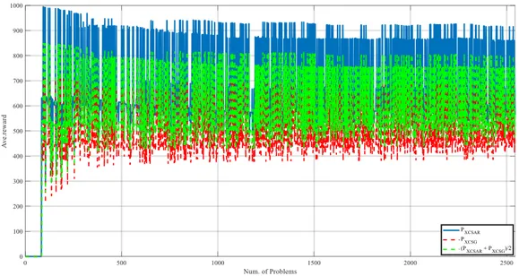
Figure 4-5: Average reward approach, discounted reward approach and maximum of these approaches applied to Environment1. ... 43

Figure 4-6: Population size in macro classifier for applying the max of XCSAR and XCSG to Environment1 ... 44

Figure 4-7:Performance of applying MIXCS to Environment2 ... 45

Figure 4-9: Population size in macro classifier for applying the competition of XCSAR and XCSG to Environment2. ... 48

Figure 4-10: Average reward approach, discounted reward approach and maximum of these approaches applied to Environment2. ... 49

(12)

LIST OF SYMBOLS AND ABBREVIATIONS

AXCS XCS with a method of average reward CASs Complex adaptive systems

GA Genetic algorithm

LCSs Learning classifier systems MDF Markov decision process

MIXCS Linear combination of XCSG and XCSAR RL Reinforcement leaning

XCS Extended classifier systems

XCSAR XCS with a method of average reward XCSG XCS with gradient

A Action space

R: S × A → ℝ Reward function S State space

T: S × A → S Transition probability function t Time step

(13)

CHAPTER 1 INTRODUCTION

1.1 Motivation

Our world is based on the interplay of different elements and factors which therefore cannot be regarded individually but rather as a whole; these systems are defined as “complex system” and have the capacity of changing and learning from experiences. A common way to describe such systems are rules, and they can represent these systems; since rules are virtually defined as an accepted means of expressing knowledge for decision making (Holmes, Lanzi, Stolzmann, & Wilson, 2002). The question arises which single best-fit model most suitable in dealing with these complex systems. One possible and powerful solution is so-called rule-based agents, agent is a single component of a given system to interact with the world as an environment of the problem domain. An intelligent agent model that interacts with the environment and improves adaptively with experience is called learning classifier system. Learning is the source of improvement and promotes the system to provide payoff from the environment (Urbanowicz & Moore, 2009). Artificial markets are a rising form of agent-based social simulation in which agents represent individual consumers, traders, firms or industries interacting under simulated market conditions. Agent-based social simulation is particularly applicable for studying macroscopic structures like organizations and markets that are based on the distributed interactions of microscopic agents. The structure of the artificial markets is designed according to agent specification, and one way to do this is the ad hoc approach. This approach is often used to explore market behaviour at a high level of abstraction. Like models that are considered for artificially intelligent agent-based social simulation that include an agent or agents which interact with environment and learn and adapt over period, here the environment is a two-dimensional grid in which the agent navigates to find the source of payoff, and where the rules govern the interaction between agents and the environment (Zenobia, Weber, & Daim, 2009).

Payoffs are considered as positive rewards, and rule-based agents aim to maximize the achieved environmental payoffs (Tesfatsion, 2000). While these simple, general models have been useful for demonstrating how complex behavioural patterns can appear from simple elemental mechanisms, their low accuracy has limited their applicability to real markets (Zenobia et al., 2009).

(14)

The artificial market needs more advanced innovation forecasting tools to study organizational phenomena (Zenobia et al., 2009) or add more parameters to calculate the accuracy of prediction (S. W. Wilson, 1995). Single models or combinations of the models are applied to help the agent to learn, adapt and take action in the environment.

“In combining the results of these two methods, one can obtain a result whose probability law of error will be more rapidly decreasing.” (Laplace, 1818)

This quote shows that combining estimates is not new. Laplace considered combining regression coefficient estimates, one being least squares and the other a kind of order statistic, many years ago. In his work, he compared the properties of two estimators and derived a combining formula. However, he concluded that not knowing the error distribution made this combination inaccessible. The topic has remained of great interest in the community, and considerable literature has accumulated over the years regarding the combination of forecasts (Clemen, 1989).

Hashem and Schmeiser propose another contribution regarding multiple models regarding using optimal linear combinations of some trained neural networks instead of using a single best network. Their results suggest that model accuracy can be improved by combining the trained networks. The vast available literature about combining models in order to obtain a certain output in very different domains motivates us to also use this approach for combining models respect to the learning classifier systems.

This leads to two main question; how to predict expected payoff of such a combined approach? Furthermore how to accurately relate the input from the environment with a corresponding action for the payoff prediction?

The solution is provided by accuracy-based fitness. XCS is a classifier where each classifier provides an expected payoff prediction. The fitness is calculated based on an inverse function of the classifier’s average prediction error. The prediction error is an average of a measure of the error in the prediction parameters. The prediction itself is an average of the payoff received that is updated by a Q-learning-like quantity and the reinforcement learning technique which discounts the future payoff received (Wilson, 1995). What method could replace Q-learning-like quantity to provide a prediction value that has a direct effect on the fitness?

(15)

The answer is R-learning. R-learning is similar to Q-learning in form; both are based on iteratively approximating the action values which represent the average adjusted reward of doing an action for the input received (Zang, Li, Wang, & Xia, 2013).

To the best of our knowledge, none of the classifier systems uses a combination of iterative approximation from the table of all action values. This study considers the simple combination of two reinforcement learning techniques to calculate the prediction of the systems and compare its result with a single reinforcement learning technique. This combination is applied in a two-dimensional grid representing an artificial trade market to see the profitable action that agent takes through navigating.

1.2 A brief overview of the proposed methodology

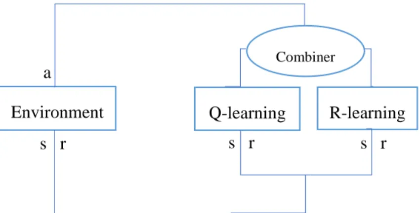
To meet the stated goal, we present the simple average of two techniques Q-learning and R-learning based on ensemble averaging to forecast the prediction of the next movement in two two-dimensional grids. They are assumed as environments, Environment1 and Environment2, where the agent should navigate to reach the considered goal. Figure 1.1 outlines this approach schematically.

Although both environments contain similar objects to represent the rules to learn through exploring and taking action to maximize the profit, they differ regarding size and the actual type of rule objects. The possible action set is divided into two parts, buy and sell, based on the location input received from the agent. The number of buying and selling for similar inputs that maximize profits is calculated. The optimum average of profit is calculated and compared against the single

s r s r

s r a

Environment Q-learning R-learning

Combiner

(16)

model approach. The average profit in the combination techniques is close to the optimum average in Environment1, and the results show that maximum profit will be reached by increasing the selling action. Also, a comparison between two single techniques is made to identify the maximum prediction. Since the considered rules in Environment1 are more straightforward than in Environment2, the agent is able to acquire enough knowledge through exploring to take the required actions, whereas the complexity of Environment2 is too high to have a similar effect. As a result, the average profit in this environment diverges greatly from the optimum value for both, the single and the combined approach.

1.3 Thesis structure

In the following chapter 2, sorrow literature is presented. chapter 3 describes the XCS algorithm developed in the course of this thesis. The performance of the proposed algorithm applied to Environment1 and Environment2 is given in chapter 4. Finally, the conclusion and outlook on the future works are presented in chapter 5.

(17)

CHAPTER 2 ARTIFICIAL MARKET, REINFORCEMENT LEARNING

AND CLASSIFIER SYSTEMS

In this chapter, the artificial market, Markov decision process and the concept of reinforcement learning, reinforcement learning in Markov decision environment, learning classifier systems and the genetic algorithm will be discussed.

2.1 Artificial market

Computer simulation has a long history in simulating organizations by the agent-based paradigm. Agent-based social simulation (ABSS) can fairly well study macroscopic structures like organizations and markets that are based on distributed interactions of microscopic agents. Artificial markets (AMs) are rising a form of ABSS where agents represent individual consumers, firms, trader or industries interacting under simulated market conditions. One of the identified promising applications of AMs in technological innovation is synthesizing and filtering useful information from massive data sets. In this application, agents represent variables and parameters of a data set. These agents will improve through positive feedback or vanish otherwise. The agents also interact and create a new generation of agents that show a higher-order interaction term. As will be shown in the following, an AM could be used to naturally select a population of variables and interaction terms that predict future market behaviour (Zenobia et al., 2009).

The underlying concept is inspired from animal life to find the basic and simple common behaviour between humans and animals when interacting with their environment. Some of these mutualities are for example adaptive behaviour for foraging, navigation and obstacle avoidance in an unknown environment as has been first discussed by Wilson in 1986 (S. W. Wilson, 1986). He offered a bottom-up approach to construct the Animat model from its primitive elements according to four basic characteristics of animals. First, only current sensory signals from the environment are essential for the animal at each moment. Second, the animal is capable of taking action to change these environmental signals. Third, certain signals have a special meaning for the animal, and fourth, the goal of the animal is to externally or internally optimize the rate of occurrence of certain signals (S. W. Wilson, 1986). Needs and satisfaction identify the agent in this model according to these four characteristics.

(18)

Based on characteristics, the agent in the Animat model is inspired by real-life rules that are shared between all types of animals, i.e. the manner of interaction with the environment. Based on the first and second characteristics they sense and connect to the environment to satisfy their need. The environment is a simulated world which contains the fundamental objects to serve the surviving task. The animal’s ecosystem inspires it. In ABSS, the surviving task of the agents is defined based on the problem, for example, acquiring maximum resources, maintaining a minimum level of energy, prey hunting, obstacle avoidance, etc.

A finite- state machine is one formal way to characterize the environment formally. Two equations define the behaviour of a finite-state machine

𝑄(𝑡 + 1) = 𝐹(𝑄(𝑡), 𝐴(𝑡)) (2-1) 𝐸(𝑡 + 1) = 𝐺(𝑄(𝑡), 𝐴(𝑡)) (2-2)

Where 𝐴 is the environment input, 𝐸 is the environment output, and 𝑄 represent the current state, time 𝑡 is assumed to be discrete. The variable 𝐴 and 𝐸 are general vectors. The first equation says that the environment’s next state is a transition function 𝐹 of its current state and its defined action. The second equation says that the simulated input at 𝑄(𝑡) for action at 𝑡. In general, the model says that the action in an environment results in a new simulated input.

The class of environment is defined depending on the state transition of an agent. If the current state determines the desired action in a state, the agent is placed in a Markovian environment. Otherwise, it needs to have a history of states, and the environment is non-Markovian (S. W. Wilson, 1991). In the next section, a Markovian environment will be discussed in detail.

Agents involved in such a system that consists of a network of interacting agents and exhibit an aggregate behaviour that rises from the individual activities of the agents. It is possible to describe its aggregated behaviour without any knowledge of the individual behaviour of the agent. An agent in such an environment is adaptive if it reaches the goal that is defined by the system. Computer-based adaptive algorithms such as classifier systems, genetic algorithm and reinforcement learning are applied to explore artificial adaptive agents (Holland & Miller, 1991).

In the artificial market, it is necessary to argue how to design the input and output of the agent (Nakada & Takadama, 2013). In this study, an agent is considered as a trader in a stock market where is depicted by two grid environments, one of this environment has a simple 5 × 5 grid cell

(19)

and the other environment 9 × 9 grid cell that every object is randomly placed. While the agent is randomly located in the environment, its interaction with the environment is analyzed. The task of the agent is to maximize the profit that is provided as Food (𝐹). The action of the agent as a trader is to sell or to buy. There are some objects that are called obstacles (𝑂), they represent the action of hold, the agent cannot trade in the vironment, but in the number of action is considered, and it should choose another action. The possible trade opportunities are demonstrated by (. ).The possible action set for this agent is 𝐴 = {1,2,3,4,5,6,7,8}, figure 2-1 shows that how the agent ∗ can move around the environment to perform its task.

8 1 2 7 ∗ 3 6 5 4

Figure 2-1: The possible actions in each state for the agent ∗

Each number shows one cell of the environment; it means that agent ∗ can have information of the eight cells at each time step; this information is agent’s knowledge that after randomly exploring to learn as much as possible about its environment. After learning the environment, the agent tries to maximize environmental reward in our case profit. In chapter 3, environments are illustrated, and the design of input and output will be explained in details.

2.2 Reinforcement learning

2.2.1 Markov decision processes (MDPs)

A deterministic MDP is defined by its state space 𝑆, its action space 𝐴, its transition probability function 𝑇: 𝑆 × 𝐴 → 𝑆, which describes how the state changes as a result of the actions, and its reward function 𝑅: 𝑆 × 𝐴 → ℝ which evaluates the quality of state transitions. The agent behaves according to the policy 𝜋: 𝑆 → 𝐴. As a result of the action 𝑎𝑡 applied in the state 𝑠𝑡 at the discrete

time step 𝑡 the state changes to 𝑠_𝑡+1 according to the transition function 𝑠_𝑡+1= 𝑇(𝑠_𝑡, 𝑎_𝑡). At the same time, the agent receives the scalar reward 𝑟_𝑡+1, according to the reward function 𝑟_𝑡+1= 𝑅(𝑠 _𝑡, 𝑎_𝑡) where ‖𝑅‖_∞ = 𝑠𝑢𝑝_𝑠,𝑎|𝑅(𝑠, 𝑎)| is finite. The reward evaluates the immediate effect of the action 𝑎𝑡, namely the transition from 𝑠𝑡 to 𝑠𝑡+1, but in general does not say anything about its

(20)

The agent chooses actions according to its policy 𝜋, using 𝑎_𝑡 = 𝜋(𝑠_𝑡). Given 𝑇 and 𝑅, the current state 𝑠𝑡 and the current action 𝑎𝑡 are sufficient to determine both the next state 𝑠𝑡+1 and the

reward 𝑟_𝑡+1. To show the Markov property, which is essential in providing theoretical guarantees about reinforcement learning algorithms, suppose 𝑋 is a random variable that can take its value 𝑋_𝑡 at time 𝑡 among the state space 𝑆 = {𝑆1, 𝑆2, … , 𝑆𝑛}. The random variable 𝑋𝑡 is a Markov chain if:

𝑃𝑟(𝑋_𝑡+1= 𝑠_𝑡+1|𝑋𝑡= 𝑠𝑡, 𝑋𝑡−1= 𝑠𝑡−1, … , 𝑋1 = 𝑠1, 𝑋0 = 𝑠0) = 𝑃𝑟(𝑋𝑡+1= 𝑠𝑡+1|𝑋𝑡= 𝑠𝑡) (2-3)

It shows the probability distribution of the state at time t+1 depends only on the state at time t (Hohendorff, 2005).

A Markov chain can be shown based on transition probability. Suppose 𝑝(𝑖, 𝑗) is the probability of going from 𝑠_𝑖 to 𝑠_𝑗 by one step, so

𝑝(𝑖, 𝑗) = Pr (𝑋_𝑡+1= 𝑠_𝑗|𝑋_𝑡= 𝑠_𝑖) (2-4) The transition probability for all state is considered as

𝜇(𝑡) = [𝜇₁(𝑡) 𝜇₂(𝑡) … ] = [Pr(𝑋_𝑡= 𝑠₁) Pr(𝑋_𝑡= 𝑠₂) … ] (2-5)

The dimension of 𝜇(𝑡) is as same as the dimension of 𝑆. All of the elements of 𝜇(0) are zero except that one the random variable is in the state. From Chapman-Klmogrov equation,

𝜇_𝑖(𝑡 + 1) = Pr(𝑋𝑡+1= 𝑠𝑖) = ∑ Pr(𝑋𝑡+1 = 𝑠𝑖|𝑋𝑡 = 𝑠𝑘) Pr(𝑋𝑡= 𝑠𝑘) 𝑘

= ∑ 𝑝(𝑘, 𝑖)𝜇_𝑘 _𝑘(𝑡) (2-6)

𝑃 is the probability transition matrix that the sum of the rows elements of 𝑃 is one. So, 𝜇(𝑡 + 1) = 𝜇(𝑡)𝑃.

A n-step transition probability 𝑝_𝑖𝑗(𝑛) is the probability of starting from state 𝑖 to state 𝑗 after n states. It means

𝑝_𝑖𝑗(𝑛) = Pr(𝑋_𝑡+𝑛= 𝑠_𝑗|𝑋_𝑡= 𝑠_𝑖) (2-7) Where 𝑝_𝑖𝑗(𝑛) is the 𝑖𝑗𝑡ℎ element of 𝑃𝑛.

A vector 𝜇 = (𝜇₁, … , 𝜇_𝑘)𝑇 is considered as a stationary distribution for the Markov chain (𝑋0, 𝑋1, …) if

(21)

𝜇 ≥ 0 ∀ 𝑖 ∈ {1, … , 𝑘} 𝑎𝑛𝑑 ∑ 𝜇_𝑖 = 1

𝑘

𝑖=1

𝜇𝑇𝑃 = 𝜇𝑇 (2-8)

The current state and next states are independent of initial condition (Hohendorff, 2005).

The reinforcement learning literature often uses “trials” to refer to trajectories starting from some initial state and ending in a terminal state that once reached, can no longer be left.

2.2.2 Definition and basic architecture of reinforcement learning

Dynamic programming (DP) and reinforcement learning (RL) are two algorithmic methods that are applied to solve problems in which actions are used to a system over a period, the time variable is usually discrete, and actions are taken at every discrete time step, to receive the desired goal. DPs methods need to assume the model is known whereas RL methods only require to have access to a set of samples. DPs know the transition probabilities and the expected immediate reward function. Both of these models are useful to obtain behaviour for intelligent agents. If the model of the system cannot be obtained, RLs methods are helpful; since they work using only data obtained from the system without requiring a model of its behaviour (Busoniu, Lucian, et al., 2010).

Reinforcement learning is the problem faced by an agent that must learn how to behave through trial-and-error interactions with an environment. The goal of reinforcement learning is to maximize the rewards and minimize the punishments the agents receive. From the psychological point, the idea of reinforcement learning is inspired by doing the action for a belated reward by animals and human (Richard S. Sutton, 2017).

The main elements of reinforcement learning problems are states (situations), actions that each action influences the agent’s future state and payoffs (rewards or punishments in reinforcements). The agent can take action among the set of possible actions based on a given state, then the agent may transition to a new state and may receive payoffs.

(22)

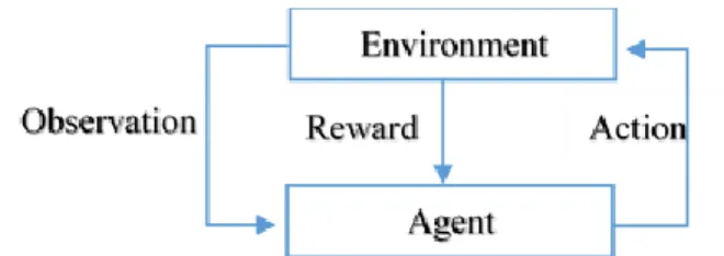
Figure 2-2: Block diagram of the reinforcement learning problem

In this diagram, first, the agent observes the current state of the environment and then chooses an action among the possible action set. In the next step, it receives the immediate reward for its action. To receive the goal of maximization of reward, the agent should try to learn in several times. The agent finds the rule of choosing an action at each state of the environment; this rule is called policy.

More formally, an agent moves in an environment which is characterized by a set S of state, and for each set of state 𝑠 ∈ 𝑆 there is a set of possible actions 𝐴(𝑠_𝑡) at a discrete time step t=0, 1, 2…. According to the observed state, the agent chooses an action 𝑎𝑡 ∈ 𝐴(𝑠𝑡). In the next step, t+1 the

agent will receive a reward 𝑟_𝑡+1∈ 𝑅 in the state of st+1. The agent’s goal is to maximize long- term

reward, which is defined as the discounted sum of future rewards:

∑∞_𝑡=𝜏𝛾𝑡−𝜏𝑟_𝑡 0 ≤ 𝛾 < 1 (2-8)

Coefficient 𝛾 is the discount factor which determines the importance of later and sooner reward. The agent chooses the action according to a policy, the policies are shown by π. If the policy is nondeterministic, giving more actions for a same state, is presented by the probabilistic mapping that is shown, 𝜋_𝑡(𝑠, 𝑎) that represents 𝑎_𝑡 = 𝑎 if 𝑠_𝑡= 𝑠. If the policy is deterministic, there is a single action for each state and it is shown by π(s). For each state, an optimal policy gives the best action to perform in that state. When the agent found an optimal policy, it must follow that policy to behave optimally (Maia, 2009).

Since an action effects on the immediate reward, the value of the next state is beneficial to know. In other words, determining the values of states can help in solving the problem. The state- value function, 𝑉𝜋_{(𝑠) is the expected value of the discounted sum of future reward when the agent starts}

from s and follows the policy π.

(23)

The total expected reward when the agent is in the state 𝑠_𝑡= 𝑠, perform action 𝑎, and transition to state 𝑠′ is divided to two parts, immediate reward [𝑅(𝑠, 𝑎, 𝑠′)] and discounted reward when the state 𝑠′_{starts 𝛾[𝛾𝑉}𝜋_(𝑠′_{)]. The average of the sum of these presented rewards give the value of the}

state. In mathematical form:

𝑉𝜋_{(𝑠) = ∑} _{𝜋(𝑠, 𝑎) ∑ 𝑇(𝑠, 𝑎, 𝑠}′_{). [𝑅(𝑠, 𝑎, 𝑠}′_{) + 𝛾𝑉}𝜋_(𝑠′_)] 𝑠′

𝑎∈𝐴(𝑠) (2-10)

The equation (2-10) is known as the Bellman equation (Maia, 2009). 2.2.3 Reinforcement learning in Markov environment

The problem of reinforcement learning is formalized by using the ideas from dynamical systems theory as the optimal control of Markov decision processes. In dynamic programming (DP) as same as the reinforcement learning, an agent interacts with the environment by the received state, which describes the state of the environment, an action among possible action set, and a scalar reward which provides the feedback on immediate performance. DP and RL problems can be formalized with the help of MDPs (Busoniu, Lucian, et al., 2010).

MDPs straightly indicates the frame of the problem of learning from interaction to achieve a goal. MDPs are a mathematical form of reinforcement learning problem for which precise theoretical statement can be made.

The agent and environment interact at each time steps, 𝑡 = 0,1,2,3, …. The agent receives input from the environment’s state 𝑠𝑡 ∈ 𝑆, based on selects an action 𝑎𝑡 ∈ 𝐴. One time step later, the

agent receive a numerical reward 𝑟_𝑡+1∈ 𝑅, as the consequence of its action, then the agent will be in a new state 𝑠_𝑡+1. This is the trajectory of MDP. To show the mathematical expression of a reinforcement problem in Markov transition probability and the expected value of the next reward:

𝑃(𝑠′|𝑠, 𝑎) = 𝑃𝑟(𝑠𝑡+1= 𝑠′|𝑠𝑡= 𝑠, 𝑎𝑡 = 𝑎) (2-11)

𝑅(𝑠, 𝑎, 𝑠′_{) = 𝐸(𝑟}

𝑡+1|𝑠𝑡 = 𝑠, 𝑎𝑡= 𝑎, 𝑠𝑡+1= 𝑠′) (2-12)

Transition probability 𝑃(𝑠′|𝑠, 𝑎) is the probability of state changes from 𝑠 to 𝑠′_{given action 𝑎. The}

expected value of the next reward 𝑅(𝑠, 𝑎, 𝑠′) is the average of receiving a reward in changing from 𝑠 to 𝑠′_{given action 𝑎. The definition of 𝑃(𝑠}′_{|𝑠, 𝑎) and 𝑅(𝑠, 𝑎, 𝑠}′_{) specify the dynamic of a MDP}

(24)

The other main element of a reinforcement learning problem except agent and environment is a policy. A policy defines the learning behaviour of an agent at a given time. A policy 𝜋: 𝑆 → 𝐴 is a mapping from perceived states of the environment to action set at a given time, it is shown by 𝜋_𝑡(𝑠, 𝑎). To compute the optimal policies for a MDP, dynamic programming is used. The goal of both DP and RL is to find an optimal policy that maximize the return from any initial state 𝑠0.

The return is a cumulative aggregation of rewards along a trajectory starting at 𝑠₀. The finite-horizon discounted return is given by ∑ 𝛾𝑡_𝑟

𝑡+1= ∑𝑇𝑡=0𝛾𝑡𝑅(𝑠𝑡, 𝜋(𝑠𝑡)) 𝑇

𝑡=0 .It represents the reward

obtained by the agent in the long run. Based on the way of accumulating the rewards, there are several types of return.

A convenient way to characterize policies is to define their value functions. There are two types of value function: state-action value functions and state value functions.

1. State-action value function

The state-action value function 𝑉𝜋_{: 𝑆 × 𝐴 → ℝ of a policy 𝜋 gives the return obtained when starting}

from a given state, applying a given action, and following 𝜋 thereafter: 𝑉𝜋_{(𝑠, 𝑎) = 𝐸}𝜋_(𝑅

𝑡|𝑠𝑡= 𝑠) = 𝐸𝜋[(∑∞𝑘=0𝛾𝑘𝑟𝑡+𝑘+1|𝑠𝑡 = 𝑠)] (2-13)

Where (𝑠₀, 𝑎₀) = (𝑠, 𝑎), 𝑠_𝑡+1= 𝑇(𝑠_𝑡, 𝑎_𝑡) 𝑎𝑛𝑑 𝑎_𝑡 = 𝜋(𝑠_𝑡). Then, the first term is separated and the rest of the equation is written in a recursive from

𝑉𝜋(𝑠, 𝑎) = 𝑅(𝑠, 𝑎) + 𝛾𝑅𝜋_{(𝑠, 𝑎, 𝑠}′₎ _(2-14)

The optimal value function is defined as the best value function that can be obtained by any policy: 𝑉∗(𝑠, 𝑎) = max

𝜋 𝑉

𝜋_{(𝑠, 𝑎)} _(2-15)

Any policy 𝜋∗_{that selects at each state an action with largest optimal value, i.e., that satisfies:}

𝜋(𝑠) ∈ 𝑎𝑟𝑔𝑚𝑎𝑥𝑣∗(𝑠, 𝑎) (2-16)

In general, for a given value function that satisfies (2-16) condition is said to be greedy.

𝑉𝜋 and 𝑉∗ are recursively characterized by Bellman equations, which are of central importance for value iteration and policy iteration algorithms. The Bellman equation for 𝑉𝜋_{states that the value}

of taking action 𝑎 in state 𝑠 under the policy 𝜋 equals the sum of the immediate reward and the discounted value achieved by 𝜋 in the next state:

(25)

𝑉𝜋_{(𝑠, 𝑎) = 𝑅(𝑠, 𝑎) + 𝛾𝑅}𝜋_{(𝑇(𝑠, 𝑎), 𝜋(𝑇(𝑠, 𝑎))} _(2-17)

The Bellman optimality equation characterizes 𝑉∗, and states that the optimal value of action 𝑎 taken in state 𝑠 equals the sum of the immediate reward and the discounted optimal value obtained by the best action in the next state:

𝑉∗_{(𝑠, 𝑎) = R(s, a) + 𝛾 max} 𝑎′ 𝑉

∗_{(𝑇(𝑠, 𝑎), 𝑎}′₎ _(2-18)

2. State value function :

The state value function 𝑉𝜋_{: 𝑆 → ℝ of a policy 𝜋 is the return obtained by starting a particular state}

and following 𝜋. State value function can be computed from 𝑉𝜋(𝑠) = 𝑉𝜋_{(𝑠, 𝜋(𝑠)). The optimal}

state value function is the best state value function that can be obtained by any policy, and can be computed from the optimal 𝑉∗(𝑠):

𝑉∗(𝑠) = max

𝜋 𝑉

𝜋_(𝑠) _(2-19)

An optimal policy 𝜋∗_{can be computed from 𝑉}∗_{by suing the fact that it satisfies:}

𝜋∗_{(𝑠) ∈ argmax} 𝑎

[𝑅(𝑠, 𝑎) + 𝛾𝑣∗_{(𝑇(𝑠, 𝑎))]} _(2-20)

The 𝑉𝜋_{and 𝑉}∗_{satisfy the Bellman equations (Busoniu, Lucian, et al, 2010),}

𝑉𝜋_{(𝑠) = 𝑅(𝑠, 𝜋(𝑎)) + 𝛾𝑉}𝜋_{(𝑇(𝑠, 𝜋(𝑠)))} _(2-21)

𝑉∗(𝑠) = max

𝑎 [R(s, a) + 𝛾𝑉

∗_{(𝑇(𝑠, 𝑎))]} _(2-22)

2.2.4

Temporal differences

Since the agent does not know the MDP, temporal difference learning estimates 𝑉𝜋_{(𝑠) by taking}

the observed value of 𝑅(𝑠, 𝑎, 𝑠′) + 𝛾𝑉𝜋_(𝑠′_{) as a sample. In a statistical point of view, the agent}

likely selects action 𝑎 after many times to visit state 𝑠 with probability 𝜋(𝑠, 𝑎). In the same way, the agent chooses a state 𝑠′ with the transition of 𝑇(𝑠, 𝑎, 𝑠′). So, there is an estimate of 𝑉𝜋(𝑠) that is shown by 𝑉̂𝜋(𝑠), therefor 𝑅(𝑠, 𝑎, 𝑠′) + 𝛾𝑉̂𝜋_(𝑠′_).

It is essential to consider the potential changes in recent samples to estimate 𝑉𝜋_{(𝑠). The simple}

(26)

𝑥₁, 𝑥₂, … , 𝑥_𝑛 be a sequence of number and 𝑥̅_𝑛 is an exponential recency- weighted average of these numbers, 𝑥̅𝑛+1 = 𝑥̅𝑛+ 𝛼[𝑥𝑛+1− 𝑥̅𝑛] is an exponential recency-weighted average of

𝑥1, 𝑥2, … , 𝑥𝑛, 𝑥𝑛+1 (Maia, 2009). So, it is possible to update 𝑉̂𝜋(𝑠),

𝑉̂𝜋_{(𝑠) ← 𝑉̂}𝜋_{(𝑠) + 𝛼[𝑅(𝑠, 𝑎, 𝑠}′_{) + 𝛾𝑉̂}𝜋_(𝑠′_{) − 𝑉̂}𝜋_{(𝑠)] (2-23)}

The prediction error is defined by the difference between the sample of the discounted sum of future reward and one that is predicted. It is presented as following

𝛿 = 𝑅(𝑠, 𝑎, 𝑠′_{) + 𝛾𝑉̂}𝜋_(𝑠′_{) − 𝑉̂}𝜋_{(𝑠) (2-24)}

A form of (2-23) based on prediction error is:

𝑉̂𝜋(𝑠) ← 𝑉̂𝜋_{(𝑠) + 𝛼𝛿 (2-25)}

𝑉̂𝜋(𝑠) ← (1 − 𝛼)𝑉̂𝜋_{(𝑠) + 𝛼[𝑅(𝑠, 𝑎, 𝑠}′_{) + 𝛾𝑉̂}𝜋_(𝑠′_{)] (2-26)}

Also, this form indicates the new estimate of 𝑉̂𝜋_{(𝑠) is a weighted average of the old estimate and}

the provided estimate by the current sample. 2.2.5 Q-Learning

The Bellman optimality equation is applied by value iteration techniques to iteratively compute an optimal value function, form which an optimal policy is derived. Q-learning, the most wildly used algorithm from model-free value iteration algorithm. Q-learning begins from an arbitrary initial value and updates it without requiring a model. Instead of a model, Q-learning uses state transitions and rewards, a data tuples 𝑠_𝑡, 𝑎_𝑡, 𝑠_𝑡+1, 𝑟_𝑡+1. This is the simple way to find a policy and value function is to store action value 𝑄(𝑠, 𝑎) for each state 𝑠 and action 𝑎 (Watkins & Dayan, 1992). After each transition, the Q-function is updated by using a data tuple, as follows:

𝑄_𝑡+1(𝑠_𝑡, 𝑎_𝑡) = 𝑄_𝑡(𝑠_𝑡, 𝑎_𝑡) + 𝛼[𝑟_𝑡+1+ 𝛾 max

𝑎′ 𝑄𝑡(𝑠𝑡+1, 𝑎

′_{) − 𝑄}

𝑡(𝑠𝑡, 𝑎𝑡)] (2-27)

where 𝛼 is a learning factor, a small positive number. The term between square brackets is the temporal difference, the difference between the updated estimate 𝑟_𝑡+1+ 𝛾 max

𝑎′ 𝑄𝑡(𝑠𝑡+1, 𝑎

′_{) of the}

optimal Q-value of (𝑠_𝑡, 𝑎_𝑡) and the current estimate 𝑄_𝑡(𝑠_𝑡, 𝑎_𝑡). The other form of this updating is: 𝑄_𝑡+1(𝑠_𝑡, 𝑎_𝑡) = (1 − 𝛼)𝑄_𝑡(𝑠_𝑡, 𝑎_𝑡) + 𝛼[𝑟_𝑡+1+ 𝛾 max

(27)

The value of Q is unchanged for all other combination of 𝑠 and 𝑎. This method is a form of value iteration, one of the normal dynamic programming algorithms. According to Watkin and Dayan, this method will converge rapidly to the optimal action- value function for finite Markov decision process. He proofs Q-learning converges with probability one under an artificial controlled Markov process called the action replay process (ARP) which is constructed from the trajectory sequence and the learning rate sequence (Watkins & Dayan, 1992).

2.2.6 R-Learning

Before presenting R-learning, it is crucial to introduce the average reward optimality criteria. As it is mentioned in Q-learning section, receiving rewards in the future are geometrically discounted by the discount factor. The average reward model is an undiscounted reinforcement learning that is supposed to take actions to maximize long-run average reward per time step.

𝜌 = 𝜌(𝑠) = lim

𝑁→∞

𝐸(∑𝑁−1𝑡=0 𝑟𝑡(𝑠))

𝑁 (2-29)

Since it is supposed to calculate 𝜌 for the 𝑁 period, the upper bound of the summation is considered based on 𝑁 − 1 previous steps. We expect that the long-run average reward 𝜌 is gained by

lim

𝑁→∞𝐸(∑ (𝑟𝑡(𝑠)) 𝑁−1

𝑡=0 ) (2-30)

To show the long-run time for future reward 𝑁 → ∞ is considered.

R-learning is a similar technique to Q-learning in form. R-learning is based on iteratively approximating all action values, the more common points of these methods will be mentioned. R-learning represents the average adjusted reward of doing an action 𝑎 in state s and related policy to reach the maximize reward. Following rule shows the update R value:

𝑅_𝑡+1(𝑠𝑡, 𝑎𝑡) = (1 − 𝛽𝑅)𝑅𝑡(𝑠𝑡, 𝑎𝑡) + 𝛽𝑅[𝑟𝑡+1+ max

𝑎 𝑅𝑡(𝑠𝑡+1, 𝑎) − 𝜌] (2-31)

Here, it should update the average reward 𝜌 according to the following rule: 𝜌 = (1 − 𝛽_𝜌)𝜌 + 𝛽_𝜌(𝑟_𝑡+1+ max

𝑎∈𝐴 𝑅𝑡+1(𝑠𝑡+1, 𝑎) − max𝑎∈𝐴 𝑅𝑡(𝑠𝑡, 𝑎)) (2-32)

here, 0 ≤ 𝛽_𝑅 ≤ 1 is the learning rate for updating action values R (.,.), and 0 ≤ 𝛽_𝜌 ≤ 1 is the learning rate for updating reward 𝜌 (Zang et al., 2013).

(28)

2.3

Learning classifier systems 2.3.1 Introduction

Our world and many systems consist of interconnected parts so that some properties are not defined by the properties of individaul parts. These “complex systems” show a large number of interacting components, whose collective activity is nonlinear. One of the features of these systems is their ability to become adaptive; meaning that they can change and learn from experiences. Therefore, these systems are called complex adaptive systems (CASs). Rule-based agents represent them; the term agent is used to refer to a single component of a given system generally. In general, CASs might be seen as a group of interacting agents where a collection of simple rules can represent each agent's behaviour. These rules typically are demonstrated by “If condition Then action.” Rules generally use information from the system’s environment to make decisions.

2.3.2 What is a learning classifier system and how does it work?

Knowledge of the problem domain describes the learning classifier systems (LCSs) algorithm; this algorithm is seeking a single best-fit model when dealing with the complex systems. The LCSs outputs are classifiers to model an intelligent decision maker collectively. In general, a LCS is an intelligent agent model that interacts with an environment and improves adaptively with experience. The algorithm improves by reinforcement due to payoff by the environment. A LCS aims to maximize the achieved environmental payoffs.

Adaptivity and generalization are two characters that support learning classifier systems. Because of changing situations, LCS has always been viewed as adaptive systems. In recent years, there is some evidence in a different domain such as computational economics to prove this characteristic (Tesfatsion, 2000). In LCSs, generalization is achieved through the evolution of general rules; it means that a classifier can match more than one input vector of the environment. Different situations are maybe recognized with similar consequences. Scalability is the other characteristic of learning time and system size in a different environment that there is no clear answer (Holmes et al., 2002).

The four components of LCSs consist of

1) a finite population of condition-action- rules that called classifiers that represent the current knowledge of the system,

(29)

2) a performance component, which regulates the interaction between environment and classifier population,

3) a reinforcement component or credit assignment component which distributes the reward received from the environment to the classifiers and 4) a discovery component which uses different operators to discover better rules and improve existing one. These component represent an algorithmic framework.

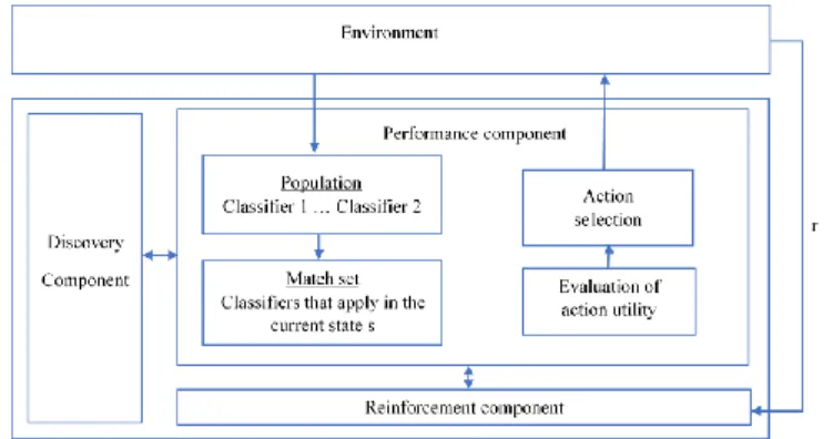
Figure 2-3: The learning classifier systems and environment

2.3.3 The discovery mechanisms and learning mechanisms

The four components of LCSs represent an algorithmic framework, and these mechanisms are responsible for driving the system. For driving the system, discovery and learning are two responsible mechanisms. Discovery mechanism refers to the rule that does not exist in the population, and each rule offers a better rule to get the payoff. Learning is a process to build a general model through experiences by interacting with the environment.

2.3.3.1 Discovery

As it mentioned, the discovery mechanism refers to rule discovery that does not exist in the population, and each rule offers a better rule to get the payoff. Making a good decision have been achieved by a genetic algorithm (GA). The GA is a computational search technique, which manipulates a population of rules to represent a potential solution to a given problem. GA is applied to classifier systems to evolve rules and create new rules that are called evolution. LCSs can be

(30)

used to solve reinforcement learning problems, classification problems, and function approximation problems (Urbanowicz & Moore, 2009).

Two measures, the prediction and fitness, are associated with classifiers. Prediction estimates the classifier utility if the classifier is used and fitness estimates the quality of the information about the problem that classifier gives, and it is exploited by the discovery component to lead evolution. Unlike the low fitness, the high fitness gives useful information about the problem, and therefore it should reproduce more through the genetic algorithm.

On each discrete time step, the system receives as input the current state of the environment 𝑠 and the match set is formed out of classifiers in the population whose condition matches 𝑠. Then, the system evaluates the prediction of the actions in the match set, an action 𝑎 is selected from those in the match set according to certain criterion and set to the environment to be performed. The system receives a reward 𝑟 according to 𝑠 and 𝑎. The reinforcement component is implanted with the discovery component, the genetic algorithm, randomly selects two classifiers from the population based on their fitness; the genetic algorithm applies crossover and mutation generating two new classifiers (Holmes et al., 2002).

There are three basic genetic operators, selection, crossover, and mutation that recombine the selected condition part of a classifier to make a new classifier for the next steps. The general algorithmic description of the genetic algorithm is as follow (K. Deb, 1999):

- Initialize parameters

- Make the initial population and fitness - Repeat:

Selection of parents to produce offspring (Reproduction) Crossover

Mutation

Updates population and fitness of individuals - End after meeting the condition

(31)

There are some methods such as tournament selection, ranking selection, and proportionate selection to identify good (usually above average) solutions in the population and eliminate the under average resolutions and replace them by copies of good answers.

Crossover operator takes a part of picking two solutions that called parent solutions from the new

population that created after selection and exchange between these picking selections. For example, A and B are two parent strings (condition) that are chosen by length five from the population,

𝐴 = 𝑎1𝑎2𝑎3𝑎4𝑎5

𝐵 = 𝑏₁𝑏₂𝑏₃𝑏₄𝑏𝑎₅

If the single-point crossover operator, where this is performed randomly choosing a crossing site along the string and by exchanging all bits on the right side of the crossing site, is 3, the resulting strings are two offspring 𝐴′ and 𝐵′:

𝐴′= 𝑏1𝑏2𝑏3𝑎4𝑎5

𝐵′_{= 𝑎}

1𝑎2𝑎3𝑏4𝑏𝑎5

Mutation operator is applied to make random changes with low probability. This operator can

change one bit of string (condition) 0 𝑡𝑜 1 or vice versa. The mutation is to keep diversity in the population.

In the learning classifier systems, GA performs on the population of classifiers. Two classifiers are selected and copied from the population with a probability proportional to their fitness. The crossover operator performs on the selected classifiers from the single-point. Then the mutation performs on the resulting classifiers. The GA produces classifiers with new conditions and new fitness values to be applied as input and make general rules in the learning classifier systems. The GA in XCS starts by checking the action set to see if the GA should be applied at all. To implement a GA the average period since the last GA application in the set must be greater than the considered threshold. Next, two-parent classifiers are selected by different selection methods such as roulette wheel selection based on fitness and the offspring are created out of them. Then, the offspring are likely crossed and mutated. If the offspring are crossed, their prediction, error and fitness (will be in details explained in the next chapter) values are set to the average of the parent’s value. Finally, the offspring are inserted in the population, followed by corresponding deletions (Butz & Wilson, 2002). The RunGA function that written in MATLAB is presented in Appendix.

(32)

2.3.3.2 Learning

Learning is a process to build a general model through experiences by interacting with the environment. This concept of learning via reinforcement is a crucial mechanism of the LCS architecture. The terms learning, reinforcement, and credit assignment are often used interchangeably within the literature. Each classifier in the LCS population contains condition, action and one or more parameter values such as fitness associated with it. These parameters can identify useful classifiers in obtaining future rewards and encourage the discovery rules (R. J. Urbanowicz and J. H. Moore, 2009). A learning agent must be able to sense the input from the environment to take actions by considering the goal or goals relating to the state of the environment. Based on the literature, some essential learning techniques for a learning agent are as follows: Supervised learning is learning from a labelled training set that provided by a knowledgeable external supervisor. Each example consists of an input object and desired output value. In another word, each case is a description of a situation with a specification of the correct action that the system should take to that situation. The objective of this kind of learning is to generalize a rule for acting correctly in situations not present in the training set.

Unsupervised learning is learning from unlabeled data; this kind of learning is typically about finding a hidden structure in the collection of unlabeled data.

Reinforcement learning is different from supervised and unsupervised learning; in interactive problems, supervised learning is often impractical to obtain proper behaviour which agent has to act. Also, reinforcement learning is trying to maximize a reward signal instead of trying to find a hidden structure. So, reinforcement learning is considered as a third machine learning paradigm, beside the other paradigm as well (Richard S. Sutton, 2017).

2.3.4 Learning classifier systems and eXtended classifier systems

Learning classifier systems is an algorithm to seek a single best-fit model to maximize the achieved environment payoffs. The replacement of the strength parameter by new attributes to classifier systems causes LCSs identifies the paradigm that proposed by Holland. One the most studied and the most applied LCSs is eXtended classifier systems (XCS) (Holmes et al., 2002). The XCS classifier systems were first presented by Stewart Wilson (Wilson, 1987) which is the top of the

(33)

research for developing a new LCS. XCS keeps all the main ideas of the previous model while it introduces some fundamental changes. In the next chapter, XCS will be discussed in details.

(34)

CHAPTER 3 XCS CLASSIFIER SYSTEM AND ENSEMBLE

AVERAGING

This chapter is divided into three parts. In the first part, XCS, the second part, ensemble averaging, methodology and the third part environments are respectively discussed in details.

3.1 XCS classifier system 3.1.1 Introduction

In classical classifier systems, the classifier strength parameter is applied as a predictor of future reward and as the classifier’s fitness for the genetic algorithm (GA). Since predicted reward cannot accurately represent fitness, XCS is a developed learning classifier systems (LCS) to overcome the dissatisfaction with the behaviour of classical learning classifier systems. While prediction of expected payoff maintains in each classifier in XCS, the fitness is a separate number base on an inverse function of the classifier’s average prediction error, a measure of the accuracy of the prediction (S. W. Wilson, 1995).

Changing the definition of fitness upon the accuracy of a classifier’s reward prediction is one of two changes to XCS. The other difference is to execute the genetic algorithm in a niche, means a set of environment states each of which is matched by the same set of classifiers, instead of panmictic (S. W. Wilson, Wilson, Xcs, & System, 1998). If there is a panmictic GA, each classifier has an equal probability of crossing with any other classifier in classifier population [P], classifiers have the same strength (S. W. Wilson, 1994). These changes in XCS shift it to accuracy-based fitness and make it superiority to traditional classifier systems. The result of a combination of accuracy-based fitness and niche GA is maximally general, complete and accurate mapping from input space and actions to payoff predictions, 𝑆 × 𝐴 ⟹ 𝑃 (S. W. Wilson, 1995).

3.1.2 Description of XCS

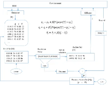
Figure 3-1 gives a view of the interaction of XCS which consist of an environment by using detectors for sensory input and effectors for motor actions. Also, the environment at the time offers a scalar reinforcement as a reward (S. W. Wilson, 1995). This figure shows the similarities of classical LCS and XCS in matching sensory information and the condition of classifiers in the population. Selecting an action based on the strategy that is applied by matched classifiers, and

(35)

turning back the effect of action to the environment by a payoff to update the population of classifiers and increase the knowledge of the system about the problem.

Figure 3-1: A detailed block diagram of XCS

XCS interacts with the environment by detectors to receive information and perform an action by effectors in the environment, and at each time step, it receives a delayed scalar payoff from the environment. In figure 3-1, [𝑃] is the population set that contains the all population of classifiers. Each classifier has two parts condition and action that take place left and right side respectably and are separated by “:”. Three values of prediction 𝑝, prediction error 𝜖 and fitness parameter 𝐹 are associated to each classifier. 𝑁 shows the maximum size of [𝑃] are randomly generated.

3.1.3 Performance component and a reinforcement component

At each time step, match set [𝑀] is created out of the current population then a prediction system for each action in [𝑀] is formed to propose the executed action (Butz & Wilson, 2002). The task of covering is to generate a classifier with a matching condition and a random action when none of the classifiers in the population match the input (Stewart W, 2007). In the next step, the prediction array [𝑃𝐴] is modified out of a match set to predict the resulting reward for each possible action. Based on [𝑃𝐴], one action is chosen for execution and action set [𝐴] is formed. Then the action with high accuracy is executed and previous action set [𝐴]−1 is modified by using the

Q-learning-like reward which is a combination of the previous reward and the largest action prediction in [𝑃𝐴]. Each classifier keeps its knowledge about the problem that received from the environment as input by detectors. Generally, each classifier is a condition-action-prediction rule that respectively are

(36)

i) 𝐶 ∈ {0, 1, #}𝐿_{determines the input states, “#” a “don’t care” symbol to permit the}

formation of generalization. This symbol shows no tendency or theoretical reason for accurate generalizations to evolve. L is a number of bit in each situation.

ii) 𝐴 ∈ {𝑎₁, … , 𝑎_𝑛} presents the action that the classifiers propose.

iii) p estimates the payoff expected if the classifier matches and its action is taken by the system (Butz & Wilson, 2002).

New classifier parameters consist of prediction 𝑝_𝑗, error 𝜀_𝑗, and fitness 𝐹_𝑗. The prediction 𝑝_𝑗 is a statistic estimating the Q- learning-like P when that classifier matches, and its action is chosen by the system. 𝑃 is updated by adding the discounted maximum of 𝑃(𝑎𝑖) of the prediction array by

multiplying discount factor 𝛾 where 0 < 𝛾 < 1 and previous action time step reward. In the next section, all parameters will be completely explained. Also, the updated parameters will be studied to see the parameter’s influence on the algorithm’s behavior while holding the rest of the parameters constant. 𝑃 is used to adjust the 𝑝_𝑗, 𝜀_𝑗, and 𝐹_𝑗.of the classifiers in [𝐴]₋₁ with learning parameter 𝛽. The updating process is as follows:

1. 𝑝𝑗 = 𝑝𝑗+ 𝛽(𝑃(𝑝𝑎𝑦𝑜𝑓𝑓) − 𝑝𝑗) where β is learning rate constant.

2. Additional considered parameters in a classifier are each classifier’s error (𝜀) is an estimate error of 𝑝𝑗, it is updated by 𝜀𝑗 = 𝜀𝑗+ 𝛽(|𝑃(𝑝𝑎𝑦𝑜𝑓𝑓) − 𝑝𝑗| − 𝜀𝑗),

3. The fitness (F) that its calculation is a little complicated, a fitness is updated when it is in [𝐴]₋₁. The update of this value depends on the accuracy of the classifier. There are three steps:

3.1. Calculate classifier’s accuracy 𝑘_𝑗 which based on the current value of 𝜀_𝑗

𝑘_𝑗 = {𝛼( 𝜀_𝑗 𝜀₀ ⁄ )−𝜗_𝜀 𝑗 > 𝜀0 1 𝑜𝑡ℎ𝑒𝑟𝑤𝑖𝑠𝑒

The threshold determines accurate and lowers accurate classifiers 𝜀₀ and 𝛼 that are constant to control the shape of accuracy, 𝜗 is applied in an internal function which scales error nonlinearly (Bull, 2015) (Butz & Wilson, 2002).

3.2. Calculating relative accuracy 𝑘_𝑗′ where 𝑘_𝑗′ is obtained by dividing its accuracy by the total accuracies in the set for each classifer.

(37)

3.3. Adjusting the fitness of the classifier 𝐹_𝑗 = 𝐹_𝑗 + 𝛽(𝑘_𝑗′− 𝐹_𝑗).

The rest of the components in the population are numerosity (𝑛); when a new classifier is generated, the population of classifiers is check out to search the same classifier of a new one. If any classifier with the same condition and action of the new generated classifier is available or not. If there is not the same classifier, new generated one is added to the population and one is added to numerosity, otherwise, the new one is not added to the population and one is added to the numerosity of classifier. These classifiers are called macro classifiers (S. W. Wilson et al., 1998). 3.1.4 Learning parameters in XCS

Some following parameters are used to control the process of learning:

(𝑁) is the maximum size of the population, start from an empty population, covering occurs at the beginning of a run.

(𝛽) is learning rate for 𝑝, 𝜀, 𝑓 𝑎𝑛𝑑 𝑎𝑠.

(𝛼, 𝜀0, 𝑎𝑛𝑑 𝜗) are used in calculating the fitness of a classifier. The value of them will be discussed

later.

(𝛾) is the discount factor used in multi-step problems in updating classifier predictions.

(𝜃_𝐺𝐴) is the GA threshold. When the average time since the last GA in the set is greater than 𝜃_𝐺𝐴, the GA is applied.

(𝜒) is the probability of applying crossover in the GA. (𝜇) is the probability of mutating an allele in the offspring.

(𝜃_𝑑𝑒𝑙) is the deletion threshold. The fitness of a classifier may be considered in its probability of deletion if the experience of a classifier is greater than 𝜃_𝑑𝑒𝑙.

(𝛿) specifies the fraction of the mean fitness in [𝑃] below which the fitness of a classifier may be considered in its probability of deletion.

(𝜃_𝑠𝑢𝑏) is the subsumption threshold. The experience of a classifier must be greater than 𝜃_𝑠𝑢𝑏 to be able to assume another classifier.

(38)

(𝑝_𝐼), (𝜀_𝐼) and (𝑓_𝐼) are used as initial values in new classifiers. They are close to zero.

(𝑝_{𝑒𝑥𝑝𝑙𝑟}) specifies the probability during action selection of choosing the action uniform randomly. (𝜃_𝑚𝑛𝑎) specifies the minimal number of actions that must be present in [𝑀] or covering.

(𝑑𝑜𝐺𝐴𝑆𝑢𝑏𝑠𝑢𝑚𝑝𝑡𝑖𝑜𝑛) is a Boolean parameter to test offspring for possible logical subsumption by parents.

(𝑑𝑜𝐴𝑐𝑡𝑖𝑜𝑛𝑆𝑒𝑡𝑠𝑢𝑏𝑠𝑢𝑚𝑝𝑡𝑖𝑜𝑛) is a Boolean parameter to be tested for subsuming classifiers(Butz & Wilson, 2002).

Checking the parameter values in the similar experiments is used to parameter setting. The optimal value of population size (𝑁) is highly depend on the complexity of the environment and the number of possible action. The learning rate, (𝛽), could be in the range of 0.1-0.2. The parameters (𝛼, 𝜀₀, 𝑎𝑛𝑑 𝜗), are normally 0.1, 1% and an integer greater than 1. The discount factor (𝛾) is between 0 and 1, in many problems in the literature is 0.71. The threshold (𝜃𝐺𝐴) is often in the

range 25-50. The GA parameters (𝜒) and (𝜇) are in the range 0.5-1 and 0.01-0.05. The deletion threshold (𝜃_𝑑𝑒𝑙) and (𝛿) is respectively often taken 20 and 0.1. (𝑃_#) could be around 0.33.

3.1.5 Generalization

According to Wilson, generalization means that different situation with equal consequences in the environment would be recognized by lower complexity than the raw environmental data. As it is mentioned in the previous chapter, generalization in LCS means that a classifier can be matched with more than one input vector that received from the environment (Wilson et al., 1998).

A mapping from state and action to the payoff prediction 𝑆 × 𝐴 ⟹ 𝑃 will be formed in XCS. In the family of learning classifier systems, XCS contains the classifier’s fitness that is given by a measure of the prediction’s accuracy and also executes the genetic algorithm in niches defined by match sets. This combination accuracy-based fitness and niche GA leads to accurate and maximally general classifiers. The question is that is it possible to stop over general classifiers by basing fitness on accuracy? That is, how possible classifiers would evolve to be general while satisfying the accuracy criteria? An accurate classifier is a classifier with an error less than 𝜀0 and a maximally

general classifier is a classifier that changing any 1 and 0 in its condition to # cause it is inaccurate. The niche environments have the same payoff to within the accuracy criterion, but represent

(39)

different inputs to the system; the goal is to put same payoff niches in one class in order to minimize the population’s size.

This mechanism is as follows. Consider two classifiers 𝐶1 and 𝐶2 with the same action, where 𝐶1’s condition is more general than 𝐶2, it means that 𝐶1’s condition can be generated from 𝐶2’s only by changing one or more of 0 or 1s condition to #. Also, they have the same 𝜀. Whenever 𝐶1 and 𝐶2 are in the same action set, their fitness values will be updated with the same values. Since 𝐶1 is more general than 𝐶2, the probability that 𝐶1 happens in more match sets is higher and is more productive in GA. Consequently, when 𝐶1 and 𝐶2 appear in the next step in the same action set, 𝐶1 will receive more fitness adjusted value resulting through the GA and 𝐶1 would eventualy displace 𝐶2 from the population (Wilson, 1995).

The generalization process should continue as long as more general classifiers can be formed without losing accuracy and should stop. The stopping point is controlled by 𝜀₀. So the classifier should evolve as long as they are general and still less than 𝜀₀. There is no theoretical reason for XCS’s tendency to evolve accurate, maximally general classifiers. The reason that XCS cannot evolve to accurate generalization is to fail to eliminate over general classifiers, even though their accuracy is low. Elimination depends on the existence of a more accurate competitor classifier in every action set where the over general occurs. When the niches of the environment are distant, the agent cannot change niches as frequently as it needs to evolve an optimal policy. Also, the mechanism of XCS deletion of over general classifiers is very slow (Wilson, 1999).

There are some generalization method such subsumption deletion that reduces population size. In simple word, subsumption is applied to remove the classifiers that cannot add anything to the capability of learning and making a decision of systems. It is helpful to have a smaller final classifier population (Butz & Wilson, 2002). For example, assume the classifier C2=###1:4 is

accurate and maximally general in some environment. If an error is less than 𝜀₀, it is called “accurate” and if accuracy won’t be changed by exchanging 1 or 0 to # is called “maximally general”. The classifier C1=##11:4 is also accurate, but it is not maximally general, because it is

subsumed by C2. It is unnecessary evolved classifier that will be eventually deleted by GA (S. W.

Wilson et al., 1998).

Two independent subsumptions, doGASubsumption and doActionSetSubsumption, are mentioned here. First one is applied during the genetic algorithm to compare the condition of an offspring