Prediction of Pilot’s Absenteeism in an Airline Company

(1)

UNIVERSITÉ DE MONTRÉAL

PREDICTION OF PILOT’S ABSENTEEISM IN AN AIRLINE COMPANY

AMIR HOSEIN HOMAIE SHANDIZI

DÉPARTEMENT DE MATHÉMATIQUES ET DE GÉNIE INDUSTRIEL ÉCOLE POLYTECHNIQUE DE MONTRÉAL

MÉMOIRE PRÉSENTÉ EN VUE DE L’OBTENTION DU DIPLÔME DE MAÎTRISE ÈS SCIENCES APPLIQUÉES

(GÉNIE INDUSTRIEL) MARS 2014

(2)

UNIVERSITÉ DE MONTRÉAL

ÉCOLE POLYTECHNIQUE DE MONTRÉAL

Ce mémoire intitulé :

PREDICTION OF PILOT’S ABSENTEEISM IN AN AIRLINE COMPANY

présenté par : HOMAIE SHANDIZI Amir Hosein

en vue de l’obtention du diplôme de : Maîtrise ès sciences appliquées a été dûment accepté par le jury d’examen constitué de :

M. FRAYRET Jean-Marc, Ph.D., président

M. AGARD Bruno, Doct., membre et directeur de recherche

M. PARTOVI NIA Vahid, Doct., membre et codirecteur de recherche M. GAMACHE Michel, Ph.D., membre et codirecteur de recherche M. ADJENGUE Luc, Ph.D., membre

(3)

DEDICATION

(4)

ACKNOWLEDGMENTS

This thesis is the result of a team work and I must thank all the academic and professional advisors without whom I would never be able to finish it. First of all, I would like to express the deepest appreciation to my supervisor Professor Bruno Agard who showed me the correct path of research with his immense knowledge, who also gave me the confidence of attacking hard problems. He also provided me full support and strong motivations. I had the privilege of being his student and benefit from his continuous guidance during my research and study. I could not have imagined having a better supervisor and mentor.

I would also like to offer my special thanks to my co-supervisor Professor Vahid Partovi Nia who generously spent his time for improving the thesis. His advices and critiques with his deep knowledge in theory and practice helped me getting around all obstacles of a scientific research. I wish to acknowledge the help provided by Professor Michel Gamache, my co-supervisor of the research. His encouragement, insightful comments, and his vast knowledge was a big support during research and while writing this thesis.

I had the chance of doing an internship in an airline company and got familiar with the research methods in practice. My sincere thanks also go to all the technical advisors of the project, Jerome-Olivier Ouellet, Mathieu Nonki, Olga Hormaza, Scott Richardson, and Steven Duke. Their comments and discussions improved considerably the results of this thesis. I would like to be thankful to all the other members of operational research group, Karine Lacerte, Jacques Cherrier, and Rodeler Joseph for the friendly environment that they provided and made this project as a memorable experience for me. I am particularly grateful for the assistance given by Jerome-Olivier Ouellet as the technical supervisor and manager of the project. He was the key person in making the results of this thesis applicable in the real situation and this research could not have resulted without his knowledge, support, deep understanding, and management skills.

I also thank the MITACS for the financial support of this thesis which helped me to concentrate completely on this project.

I would also like to thank all my comrades for their support, cups of tea, laughs, and everything; specially Vahid Partovi Nia, thank you for being my best friend. I owned you many things.

(5)

Last but not least, I wish to thank wholeheartedly my father, my mother, my sisters, and all my family for their support and encouragement throughout my study and in all steps of my life. They are meaning of life for me and I am so proud of having them. I could not even have started this thesis without their support and encouragement.

(6)

RÉSUMÉ

Les compagnies aériennes sont soumises aux nombreuses sources de perturbations pendant les opérations. Il est essentiel pour ce type d'industrie de prédire les origines des perturbations dans les différents niveaux de gestion pour réduire les coûts de rattrapage du calendrier. Une des sources les plus importantes et coûteuses de perturbation dans les compagnies aériennes est l’absentéisme des pilotes au moment de l’opération des vols.

Dans ce mémoire, nous nous concentrons sur l'absentéisme des pilotes pour cause de maladie. Nous proposons une méthode d'apprentissage supervisé qui est capable de prédire la somme mensuelle des heures de maladie chez les pilotes après la publication du calendrier. La méthode proposée utilise les caractéristiques du calendrier mensuel comme les variables explicatives et elle fait la prédiction en utilisant d’un algorithme itératif.

La méthode a été vérifiée avec des données réelles et une amélioration considérable a été observée dans les résultats. Pour rendre la méthode en situation réelle, nous avons créé une interface facile à utiliser comme un système d'aide à la décision. Cette interface automatise l'ensemble du processus de prédiction.

(7)

ABSTRACT

Airline companies are subject to a considerable number of disruptions during operations. It is vital for this type of industry to predict the source of disruptions in different levels of management to reduce the costs of schedule recovery. One of the most important and costly source of disruption in the airlines is absenteeism of the pilots at the time of the flights operation.

In this master thesis, we focus on the absenteeism of the pilots because of the sickness. We propose a supervised learning method which is able to predict total monthly sick hours after publishing the schedule. The proposed method uses characteristics of the monthly schedule as the explanatory variables and the prediction is made by using an iterative algorithm.

The model was tested with real data and a substantial improvement was observed in the results. For applying this method in business environment, we created a user-friendly web application as the decision support system. This application automates the whole process of prediction.

(8)

CONDENSÉ EN FRANÇAIS

L’objectif principal de ce mémoire est la création d’un système d’aide à la décision capable de prédire la somme des heures de maladie chez les pilotes d’une compagnie aérienne. Pour réaliser cet objectif, nous utilisons une méthode d’apprentissage supervisé dans laquelle l’arbre de décisions est l’outil principal de la méthodologie et les caractéristiques du calendrier mensuel sont des variables explicatives.

La base de données a deux parties : une première partie est l’historique qui décrit les caractéristiques des pairings (rotations) et aussi les événements de maladies associés à chaque pairing, et la seconde partie est le nouveau calendrier qui décrit les caractéristiques des pairings planifiés pour le nouveau mois. Notre objectif est de créer un système d'aide à la décision pour prédire la somme des heures de maladie pour le nouveau mois, (𝑠̂_{𝑖 𝑛+1}), par rapport au calendrier du nouveau mois (𝕊_{𝑖 𝑛+1}), aux caractéristiques des pairings et à l’histoire de maladies du passé (𝔻𝑖1, 𝔻𝑖2, … , 𝔻𝑖𝑛). Le processus d'apprentissage proposé suggère d'utiliser une boucle pour choisir

les meilleurs arbres de décisions.

Dans cette boucle, nous commençons par fixer un paramètre, appelé 𝑎, qui est le nombre de mois consécutifs nécessaires pour bâtir le premier arbre de décision stable. Ensuite, nous fusionnons les ensembles de données, 𝔻_𝑖1, 𝔻_𝑖2, … , 𝔻_𝑖𝑎, dans une base de données unique, notée Γ_𝑖𝑎. Dans la première étape de la boucle, un arbre de décisions est construit pour Γ_𝑖𝑎 et les prédictions des heures de maladie sont calculées pour chaque niveau de cet arbre. Ensuite, l'arbre est coupé au niveau ayant l'erreur minimum de prédiction pour le mois (𝑎 + 1). L'arbre coupé est appelé 𝔗̃𝑖 𝑎.

Cette boucle se répète pour obtenir (𝑛 − 1) arbres de décisions coupés 𝔗̃𝑖 𝑎, 𝔗̃𝑖 𝑎+1, … , 𝔗̃𝑖 𝑎+𝑛−1.

L’algorithme de cette boucle s’écrit comme suit : Choisissez 𝑎,

Considérez un ensemble vide comme l’ensemble des arbres de décision, Pour 𝑧 de 𝑎 à 𝑛 − 1 faites:

- Fusionnez 𝔻𝑖1, 𝔻𝑖2, … , 𝔻𝑖𝑧,

(9)

- Calculez la prédiction pour le mois suivant en utilisant 𝕊𝑖 𝑧+1 pour chaque niveau de l'arbre

obtenu,

- Calculez l'erreur pour le niveau,

- Coupez l'arbre au niveau ayant l'erreur de prédiction minimum, - Appelez l’arbre coupé 𝔗̃𝑖 𝑧,

- Ajoutez 𝔗̃𝑖 𝑧 dans l’ensemble des arbres de décision.

L’idée essentielle de la méthodologie est de trouver et d’utiliser les meilleurs scénarios des mois passés par rapport à l’historique de maladies chez les pilotes. À la fin de l’algorithme, nous utilisons (𝑛 − 1) arbres de décision 𝔗̃𝑖 𝑎, 𝔗̃𝑖 𝑎+1, … , 𝔗̃𝑖 𝑎+𝑛−1 et le calendrier du nouveau mois (𝕊𝑖 𝑛+1) pour

faire la prédiction des heures de maladies dans le nouveau mois (𝑛 + 1). Si nous utilisons le calendrier du nouveau mois comme l’entrée de ces arbres, ils donnent (𝑛 − 𝑎 − 1) valeurs différentes pour la prédiction de nouveau mois, 𝑠̂(𝔗̃𝑖 𝑎, 𝕊𝑖 𝑛+1), 𝑠̂(𝔗̃𝑖 𝑎+1, 𝕊𝑖 𝑛+1), …,

𝑠̂(𝔗̃𝑖 𝑛−1, 𝕊𝑖 𝑛+1). Chacune de ces prédictions est basée sur les règles d'association qui expliquent

le mieux la maladie d'un mois précédent. De cette façon, nous considérons la possibilité d'occurrence des scénarios précédents à l'avenir. Nous considérons une moyenne pondérée de ces estimations comme la prédiction pour le nouveau mois.

La méthodologie proposée a été appliquée dans une compagnie aérienne et les résultats montrent que dans la plupart des cas, les prédictions ont une erreur acceptable et la méthodologie proposée a amélioré d’au moins 13 pourcents les prédictions mensuelles de maladie pour l'année 2012 en comparaison avec la méthode actuelle de prédiction. Cette amélioration est obtenue lorsque l'on considère que le coût de sous-prédiction est égal au coût de sur-prédiction. Si l'on considère un coût de sous-prédiction 1,5 fois le coût de sur-prédiction, plus similaire à la valeur réelle du ratio de coûts dans les compagnies aériennes, l'amélioration de la prédiction augmente à 21 pourcents.

(10)

LIST OF TABLES

Table 3.1: An example of change of scheduled pairing due to a flight delay. ... 18

Table 3.2 : An example of change in scheduled pairing because of sickness. ... 19

Table 3.3: List of the attributes ... 21

Table 5.1: Descreptive statistics for each position and month ... 34

Table 5.2: Level errors for 𝔗_{1 12}. ... 46

Table 5.3: Level errors for 𝔗1 13. ... 49

Table 5.4: Different sickness estimation, model errors and similarity vector for March 2012. .... 50

Table 5.5: Sickness estimations relative to each model ... 52

Table 5.6: Comparison of annual prediction error (in hours) between current model of the airline company and new proposed model, for main positions in 2012. ... 54

(14)

LIST OF FIGURES

Figure 1-1: Crew scheduling in the airlines. ... 2

Figure 1-2: An example of pairing ... 3

Figure 2-1: Partitioning and CART ... 9

Figure 3-1 : Simplified airline process from scheduling to operations ... 17

Figure 3-2: Change of scheduled pairing due to a flight delay ... 18

Figure 3-3: Change of scheduled pairing because of sickness ... 19

Figure 4-1: Data pre-processing steps ... 23

Figure 4-2: Available datasets for predicting new month sickness. ... 25

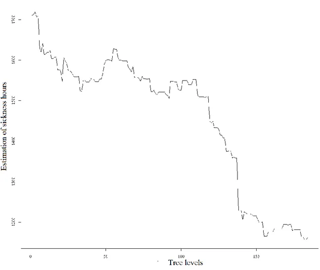
Figure 4-3: Estimation of sickness hours in different levels of the tree ... 26

Figure 4-4: Tree growing process ... 28

Figure 4-5: Prediction for the new month based on the pruned trees ... 31

Figure 5-1: Monthly sickness hours for two Positions. ... 35

Figure 5-2: Comparison between sick and non-sick pairings. ... 36

Figure 5-3: Monthly sickness percentage for Position 1. ... 37

Figure 5-4: Monthly sickness percentage for Position 2 ... 38

Figure 5-5: Mass plot for sickness, comparing total time against total credit. ... 39

Figure 5-6: Mass plot for sickness, comparing total credit against day credit. ... 40

Figure 5-7: Mass plot for sickness, comparing total credit against night credit. ... 41

Figure 5-8: Decision tree obtained from 2010 data for Position 1 ... 43

Figure 5-9: Pruning first decision tree at different levels ... 45

Figure 5-10: First decision tree that is used for predicting ... 47

Figure 5-11: Decision tree obtained from first 13 months data for Position 1. ... 48

(15)

Figure 5-13: second decision tree that is used for predicting ... 49 Figure 5-14: Comparison of model estimations, prediction and actual sickness of Position 1 in

March 2012 ... 50 Figure 5-15: Predictions versus Observation for Position 1 in 2012 ... 51 Figure 5-16: Percentage of prediction error for Position 1 in 2012 ... 53

(16)

LIST OF NOTATIONS

𝕊_𝑖𝑗 The table of pairings schedule for position i in month j. 𝕆_𝑖𝑗 The operations’ record for position i and month j.

𝔻𝑖𝑗 The database for position i and month j. The result of merging 𝕊𝑖𝑗 and 𝕆𝑖𝑗.

𝑖 As an index, denotes the position. 𝑗 As an index, denotes the month. 𝑘 As an index, denotes the pairing. 𝑙 As an index, denotes the flight leg. 𝐼_{𝑖𝑗𝑘𝑙} Flight sick indicator.

𝐶_{𝑖𝑗𝑘𝑙} Flight total credit. 𝑐_𝑖𝑗𝑘 Pairing total credit. 𝑆𝑖𝑗𝑘𝑙 Flight sick time.

𝑠𝑖𝑗𝑘 Pairing sick time.

𝑠_𝑖𝑗 Total sick time for position i in month j.

𝑦_𝑖𝑗𝑘 Response variable, sick indicator for a pairing. 𝔗 The complete decision tree

m Number of terminal nodes (regions) of 𝔗

𝓇_𝑚 Region m of a decision tree

𝓅𝑚 Probability of sickness in region m of a decision tree.

𝑐_𝑚 Total credit in region m of a decision tree. 𝓂 Number of levels of a decision tree.

𝑠̂(𝔗, 𝕊𝑖 𝑛) Sickness time prediction for pairing schedule, 𝕊𝑖 𝑛 , based on the decision tree, 𝔗.

(17)

𝑐𝑝 Cost-complexity pruning.

𝔗𝑖 𝑎 Decision tree without pruning based on Γ𝑖𝑎.

〈𝔗𝑖 𝑎〉𝓀 The pruned tree 𝔗𝑖 𝑎 at level 𝓀.

ℯ_{𝑖 𝑎𝓀} The error of prediction at level 𝓀 of the original decision tree 𝔗_{𝑖 𝑎}. 𝜂 The proportion of under-prediction cost on over-prediction cost. 𝔗̃𝑖 𝑎 Pruned decision tree based on Γ𝑖𝑎.

ℯ𝑖 𝑎 Error of 𝔗̃𝑖 𝑎 in predicting𝑠𝑖 𝑎+1.

𝜏_{𝑛 𝑎} Similarity between schedule of month 𝑎 and month 𝑛 in a specific position. 𝑠̂𝑖 𝑗 Final sick hours prediction for position 𝑖 and month 𝑗.

(18)

LIST OF AIRLINE TECHNICAL TERMS

Base The domiciles which can be considered for starting a pairing of an airline. Block holder Pilot with a flight schedule for a month, Line pilot.

Captain Responsible pilot for the flight operations and safety in an aircraft.

Deadhead A pilot who is assigned to fly as a passenger in a specific flight for transferring to duty airport. The deadhead does not pilot the aircraft. First Officer Second pilot in commercial aviation.

Leg A flight in a pairing.

Non-bidding Pilots of an airline which is neither block holder nor reserve.

Pairing Combination of consecutive flight legs which start and end at the same domicile.

PBS Preferential bidding system, a computer program that optimises airline workforce schedule.

Position Combination of aircraft type and seat.

Relief Pilot Third pilot in commercial aviation, used for long distance flights. Reserve On-call pilot for substituting the block holder in the necessary cases. Seat The seat in a flight deck which determines the arrangement of the pilots. Type of aircraft Divided categories of aircrafts for the purpose of certification.

(19)

LIST OF APPENDICES

APPENDIX A R CODES FOR WEB APPLICATION: SERVER………64

APPENDIX B R CODES FOR WEB APPLICATION: UI……….…………..70

(20)

CHAPTER 1 INTRODUCTION

In an airline company, crewing costs are second important cost after fuel costs, and pilots are the most important airline crew. Pilots are qualified for just one aircraft type as Captain, First Officer or Relief Pilot. So for big airline companies, in which there are different types of aircraft, having a good prediction of pilot absenteeism helps to manage the operations extensively.

This thesis proposes an efficient way for predicting one of the most important reasons of absenteeism, i.e. pilots’ sickness. Before starting a detailed analysis some preliminary subjects need to be explained. Chapter 1 gives a brief review of the reserve crew and crew scheduling process. Assumptions, general and specific objectives and also the structure of the thesis are also explained in this chapter.

1.1 Reserve Crew

In an airline company, in general, a pilot is qualified for one type of aircraft and one seat. The seat for the pilot, in a hierarchical rank, can be Captain, First Officer or Relief Pilot. This means a first officer of the Airbus A320 cannot be the captain of the same aircraft. The opposite is possible, but it augments the operations costs because the salary of a captain is higher than a first officer. In this study, a position is the combination of an aircraft type and a seat, e.g. 320 CA is the captain of Airbus A320.

In each month a pilot, based on his/her work schedule can be block holder, reserve or non-bidding. After publishing the monthly flight schedule, the block holders bid for determining the details of their own working schedule according to the airline’s bidding rules. Because of different unexpected conditions (such as weather conditions, pilot’s sickness, aircraft maintenance etc), it is impossible to have a fix and unchangeable schedule for monthly flights. Therefore a number of pilots are in reserve in order to take the place of the block holders when the schedule changes. It is important to have a good prediction for the number of the required reserves. A wrong number of reserves can cause two different extra operational costs for the airline company. First, if the number of reserves is greater than the number of absent pilots, the company must pay some pilots for doing nothing. Second, if the number of reserves is less than the number of absent pilots, then

(21)

the airline must pay extra for calling an out-of-duty pilot or even in the worst case it can cause the cancelation of some flights. Therefore, costs of under predictions are higher than those for over predictions.

The reserves are in backup and are used if operations could not be implemented according to the schedule. A pilot could miss his next flight because of a delay in the previous one, a change of aircraft and some other reasons can cause the use of reserve pilots. The most important reason for using the reserves in an airline is the last minute calling sick by the block holders. This covers almost 60 percent of reserves replacements in big airlines.

In this study, we focus on the prediction of absenteeism of pilots when they are calling sick. Hence, we only consider the replacements by reserves that were based on the declared sickness of pilots.

1.2 Crew Scheduling

Crew scheduling for airlines consists of different tasks. Here, we describe an introductory explanation that can help readers to follow future sections. Interested readers are referred to the text books on the airline operations such as Bazargan (2010) or Grosche (2009). For the detailed analysis of preferential bidding systems at airlines see Gamache, Soumis, Villeneuve, Desrosiers, and Gelinas (1998) and Barnhart, Belobaba, Odoni, and Barnhart (2003).

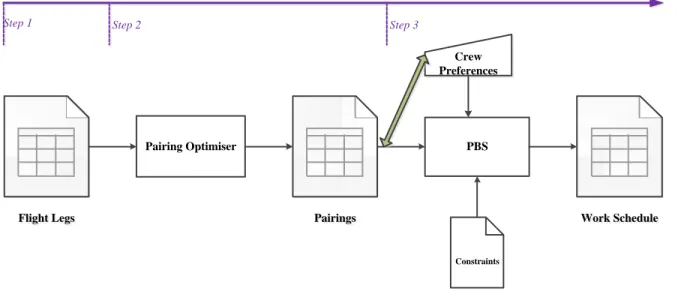
Flight Legs Flight Legs Constraints Pairing Optimiser Pairings Pairings PBS Work Schedule Work Schedule Crew Preferences Time

Step 1 Step 2 Step 3

(22)

The first step in crew scheduling process, as can be seen in Erreur ! Source du renvoi

introuvable., is publishing the list of monthly flight legs. Based on tactical and strategic decisions,

a list of flights for a business month is published by the commercial department of the airline. Each flight has its own planned characteristics such as flight departure, arrival date and time, assigned aircraft type, departure and arrival airports, flight duration, flight credits, etc.

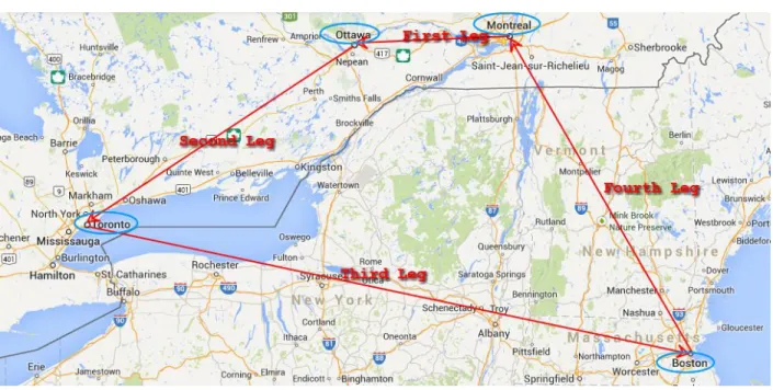
Despite other industries in which working duty consists of shifts or days, in the airlines there is an additional duty period that is called pairing. A pairing is a combination of consecutive flight legs which start and end at the same domicile (See Figure 1-2).

Figure 1-2: An example of pairing with 4 legs, started from Montreal.

The domiciles which can be considered in pairings are airline bases. Every pilot is assigned to a base for starting and finishing his own duty period. Each airline has its own bases. For example current bases for US Airways are Charlotte, Philadelphia, Washington, and Phoenix. Current bases for Air Canada are Toronto, Montreal, Vancouver, and Winnipeg.

Sometimes it is necessary to move a pilot to his duty location as a passenger because of the limitation in daily flight hours for pilots or for containing all the flight legs in the pairing list. In this case, the pilot is called deadhead and he does not pilot the aircraft.

After publishing the pairing table, in the second step, a computer program called preferential

(23)

monthly schedule and its inputs could be airline operations requirements (list of the pairings), crew

preferences (bidding) and some constraints.

After pairings are made, in the third step, bidding process starts. In the bidding process each crew requests for a certain schedule or determines his preferences. Then, the PBS assigned the list of the pairings to the pilots. This process must minimize the costs of the operations and matches aircraft type, flying routes, and pairings in a way that each pairing is assigned to only one qualified pilot. This is evident that the PBS must consider pilots’ working time and bases, such that there is no overlap in the work schedule of each pilot.

The last input for the PBS is some constraints which are legal crewing solutions that must be considered in the PBS, such as

 Government Regulations,

 Collective Bargaining Agreements,  Airline Policies.

At the end, the PBS makes the optimization based on the all explained inputs and the airline method of awarding. This method can differ from one airline to another. It could be honoring seniority in which the most senior qualified pilot for a position will be awarded by his bidding; the second will be awarded by best matches between his bidding and the remaining pairings; then the third, and so on.

1.3 Assumptions

In this study, we attack the problem of monthly sickness prediction under some minor restrictions. The predictions must be generated after publishing pairings schedule and before the bidding process because at that time the number of the reserves for the following month must be determined. For making the appropriate decision support system, we suppose that the following information exists:

 The monthly list of the pairings.

(24)

 The prediction is based on the schedule, so it does not assume changes in schedule during the operations.

 This study considers only sickness among the block holders and not the reserve pilots.  The format of all the tables that are used in making database is subject to no change.

1.4 General Objective

The general objective of this research is to develop a decision support system for predicting sickness hours in each position based on the monthly list of the pairings, in an airline company, in order to size properly the reserve crew.

1.5 Specific Objective

For achieving the goal of this project, it is necessary to define specific objectives. These specific objectives are as follows:

1- Data pre-processing: Connecting tables of schedules, bidding results and operation records to create a big data base that contains all the information, “correcting mistakes” in the data, here it seems all the data was clean.

2- Developing a method for predicting pilots’ sickness based on the history and monthly schedule of pairings.

3- Determining association rules that helps the airline managers find the characteristics of pairings in which the pilots are less interested.

4- Automating all the processes by making a user-friendly application for implementing the developed method in the business area.

1.6 Thesis Structure

The structure of the rest of the thesis is as follows. In Chapter 2, a literature review is presented. Chapter 3 describes the problem in detail. The solution approach and methodology are proposed in Chapter 4. In Chapter 5, the data pre-processing, implementation and results based on a real dataset are explained. We conclude the thesis and propose further extensions of this subject in Conclusion.

(25)

CHAPTER 2 LITERATURE REVIEW

As pilots’ absenteeism prediction is a tool for disruption management, in Section 2.1, a brief review of disruption management in airlines is presented. Section 2.2 deals with classification and regression trees which is the main statistical methodology of our prediction algorithm. Section 2.3 introduces the R packages that are used for implementing the methodology of this thesis.

2.1 Disruption Management

Unlike the strategic and tactical problems of an airline company, during flight operations most of problems must be solved in a short period of time. Therefore, managing irregular operations (disruptions) is a subject of considerable interest among many authors.

In the airline industry, disruptions can occur for several reasons: mechanical problems, weather conditions, crew sickness, security, and so on. These kinds of problems may cause flight delays or even flight cancelations. However, in many cases crew reassignment is still feasible.

One of the first works on disruption management in airline discipline was the two minimum-cost ﬂow network models presented by Jarrah et al. (1993) for absorbing the shortages. The first model chooses the set of delayed flights and the second one chooses the set of cancelations. Based on these models, a decision support system (DSS) was implemented at United Airlines and a result of valuable cost saving for using this DSS has been published (Rakshit et al., 1996).

From a different point of view, Bratu and Barnhart (2006) dealt with airline schedule recovery problem and developed an optimal trade-off between airline operations costs and passengers delay costs. They consider either passenger disruption or delay cost.

Kohl et al. (2007) discussed developing a system that uses multiple resource methods, and integrated these resources to improve the quality of decision making. They indicated that developing flexible tools must be considered in research to have added-value contribution in the businesses. They also concluded that emphasizing on finding optimum solution in the strict academic sense without weighting on the operational restrictions cannot be applicable in real situations.

Cauvin et al. (2009) proposed a multi-agent approach to the problem in a disrupted and distributed environment. Their framework proposed a way for describing the existing methods for managing

(26)

disruption. In this framework, it was necessary to identify the actors, their interactions and their consequent activities in the disruptive environment.

Disruption management in airline industry was increasingly active during the last decade, but in most of the cases the proposed solutions consider just one aspect of the problem, e.g. aircraft type, crew, passenger, etc. This is an important field of research because there is a fundamental gap between the proposed prototype tools by software companies and the ideal integrated recovery tool (Clausen et al., 2010).

A model for estimating the number of required reserve crews for covering aircraft delays callout was presented by Gaballa (1979). he minimized costs of both reserve crews and overnight delays. The application of this method resulted in a considerable cost saving at Qantas Airways.

Another example of disruption management system is an automated system that has been implemented at US Airways. This system constructs an optimal scheduling for reserve crew by emphasizing on making good reserve bid lines (Dillon and Kontogiorgis, 1999).

Wei et al. (1997) developed a modeling framework for the crew reassignment by using a heuristic branch-and-bound search algorithm. Their proposed algorithm was more flexible in comparison with the traditional operational research algorithms. They engaged the business rules to bound the solutions.

Lettovský et al. (2000) claimed that it is necessary to reduce the complexity of the problem for crew reassignment during the operations. They applied the fact that the published schedule is optimum and by using a tree-based data structure they generated the integer solutions in a short time.

RESOPT (reserve optimization) is a model developed by Sohoni et al. (2006) which effectively increases reserve availability. The model needs a good estimator for open-time reserve demand to be used as a reserve manpower controller.

Another automated decision support tool is developed by Abdelghany et al. (2004). The tool can be used in large-scale commercial airlines that use the hub-spoke network structure for crew recovering problem. A hub-spoke network is a network in which all the points are connected through spokes to the hubs instead of a point-to-point connection. This tool is flexible to different scenarios and can proactively manage the future disruptions in a chain.

(27)

2.2 Classification and Regression Tree

Classification and regression trees was presented by Morgan and Sonquist (1963) as an automatic interaction detection technique. Two decades later Breiman et al. (1984) developed the first modern and comprehensive algorithm for growing trees. Their famous method CART is a fundamental basis for classification and regression trees and the book of Breiman (1993) on the classification and regression trees is a classic reference.

For a long time, classification and regression trees (CART) have been popular for modeling and predicting among statisticians, machine learning experts and data mining practitioners. Like many other methods, these tree-based models are used when there is a response variable, 𝑌, and some predictors 𝑋₁, 𝑋₂, … , 𝑋_𝑝. Regression tree is used when the response variable is a real number while the usage of classification tree is for the cases with a categorical response. In this section, a brief introduction to classification tree is presented with a review on the literature. We consider here just binary decision tree i.e. the decision trees with a two level response variable. Although decision trees with n-level response variables, called n-ary decision tree, exist in theory and practice, we don’t consider this part of literature because the nature of our problem is binary, the pilots are either absent or present. For further reading and an in-depth discussion of this subject see Chapter 9 of Hastie et al. (2009), Chapter 6 of Wittenet al. (2011), and the classic textbook of Breiman et al. (1984).

2.2.1 Growing the tree

The main idea of tree-based models is to partition the variable space into non-overlapping rectangles and fit a constant in each partition. It is a simple but powerful idea, since any function can be approximated by piece-wise constant (step) function. Furthermore, constant model is computationally fast to fit. The fitting process requires only averaging over the response variable of observations belongs to that partition.

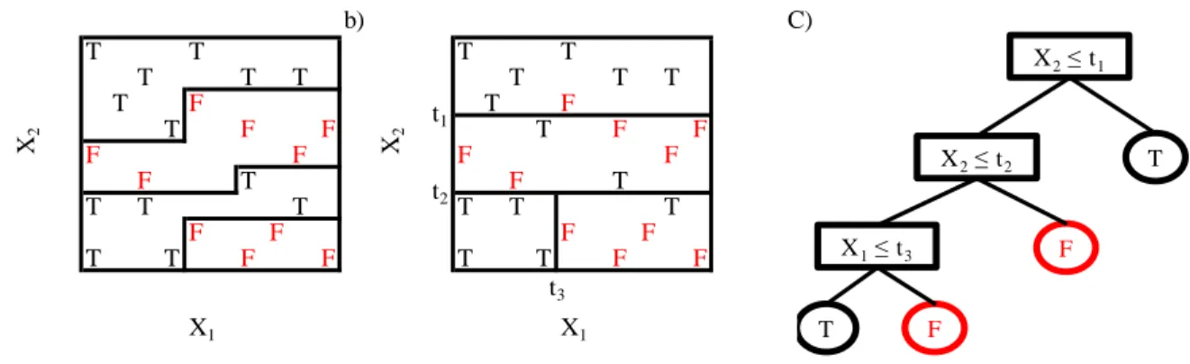
Let’s consider an example with two explanatory variables 𝑋1 and 𝑋2, each taking values in the unit

interval and a class response variable, 𝑌, which is either True (T) or False (F). As part (a) of Figure 2-1 shows, it is possible to partition the space of 𝑋₁ and 𝑋₂ so that in each subspace there exists just one kind of response: True or False. However it is difficult to determine the boundary of each region.

(28)

A partitioning like the one in Figure 2-1 (b) and its related tree structure, as shown in Figure 2-1

(c), is acceptable and applicable. The CART methodology has been developed for simplifying the

solution of this problem in an acceptable time and an efficient way with the minimum error.

Figure 2-1: Partitioning and CART. General partitioning, (a), CART partitioning, (b), and its tree representation (c).

Consider 𝑿 as the set of inputs, 𝑋₁, 𝑋₂, … , 𝑋_𝑝, and 𝑌 as the binary response variable. The goal is to find a step function like

𝑓(𝐱) = ∑ 𝑐_𝑚I(𝐱 ∈ R_m)

𝑀 𝑚=1

where 𝑀 is the number of subspaces, 𝑅_𝑚 is a subspace of the space of inputs, 𝑿. Here, 𝑐_𝑚 is the estimated constant, approximating the response variable 𝑌 in the region 𝑅_𝑚, and I(. ) is the indicator function

𝐼(𝑥 ∈ 𝑅𝑚) = {1,_0, if 𝑥 ∈ 𝑅_otherwise.𝑚

For explaining the CART algorithm, let’s start with all data, for each splitting variable 𝑗 and each split point 𝑠 we can partition the space into two subspaces,

𝑅₁(𝑗, 𝑠) = {𝑿|𝑋_𝑗 ≤ 𝑠} and 𝑅₂(𝑗, 𝑠) = {𝑿|𝑋_𝑗 > 𝑠}. Among all the input variables 𝑗 and split points 𝑠, choose the pair that

a) b) C) T T T T T T T T T T T F T F T F F T F F F F F F F T F T T T T T T T F F F F T T F F T T F F X1 X1 t1 t2 t3 X2 X2 T T F F X2≤ t1 X2≤ t2 X1≤ t3

(29)

min 𝑗,𝑠 { ∑ (𝐼(𝑦𝑖 = TRUE) − 𝑐̂1) 2 𝑥𝑖∈𝑅1 + ∑ (𝐼(𝑦_𝑖 = TRUE) − 𝑐̂₂)2 𝑥𝑖∈𝑅2 } where 𝑐̂_𝑚= 1 𝑁_𝑚 ∑ 𝐼(𝑦𝑖 = TRUE) 𝑥𝑖∈𝑅𝑚

and 𝑁_𝑚 is the number of observations in partition region 𝑅_𝑚. Now it is possible to partition the root node into two subspaces and repeat the process for each child node.

2.2.2 Splitting and Stopping Criteria

A decision tree has a hierarchical top-down order and at each node just one variable splits the space of inputs. In decision trees, the algorithm chooses a variable and a splitting point at each iteration by using an impurity measure. The splitting criteria with the stopping rule make the growing phase of the decision tree. There are two types of splitting criteria, univariate and multivariate.

Univariate splitting criteria create each node using just one variable, i.e. the discrete splitting function is univariate. These are the well known criteria that are used in almost all the famous algorithms. Information Gain (Quinlan, 1987) uses entropy measure as the impurity measure. Gini

Index (Breiman et al., 1984) is the divergence measure of the probability distribution of response

variable. Likelihood ratio chi-square statistic (Ciampi et al., 1987) in addition provides statistical inference about the information gain. Normalizing information gain by the entropy, leads to the

Gain Ratio (Quinlan, 1993). Twoing Criteria (Breiman et al., 1984) is the same as Gini Index for

binary response model and more accurate generation of it for multi-level response variable. Multivariate splitting criteria create each node by a linear combination of variables (Breiman et al., 1984) and (Sethi and Yoo, 1994). It is obvious that finding the best solution is more complicated, so multivariate splitting criteria are less popular in practice.

Another important criterion for making a tree is the stopping criteria which are applied at the end of the growing phase. Common stopping criteria are the following (Rokach and Maimon, 2005):

(30)

 The maximum tree depth reaches a pre-specified limit

 Number of cases in the node is less than a pre-specified value

 The best splitting criteria is not greater than a pre-specified threshold.

After a tree is made by using a stopping rule, it is pruned to keep the balance between bias and variance of the model for a better prediction.

2.2.3 Pruning Methods

One of the problems that occurs after growing the tree is the over-fitting, i.e. the training accuracy is high while prediction accuracy is low. In other words, the tree models the data set perfectly, but the fitted model does not work properly for predicting new observations. The reason of this problem is the over-complexity of the model and for simplifying it, pruning is necessary (Bohanec and Bratko, 1994).

There are two types of pruning. First, when it is a part of the tree construction and it is called

pre-pruning. Second, if the pruning is a separate procedure after the growing phase it is called post-pruning (Esposito et al.,1997).

There are many pruning methods (Rokach and Maimon, 2005). Among them cost-complexity

pruning (𝑐𝑝) is the most popular one. The 𝑐𝑝 is a post-pruning method proposed by Breiman et al.

(1984). In this method, all trees extracted from the original one 𝑇₀ to the root 𝑇_𝑘 are created and the best pruned tree is selected with considering the estimation of generalization error.

Let 𝑇 be a subtree of 𝑇₀ which is obtained by pruning 𝑇₀. If |𝑇| denotes the number of terminal nodes in 𝑇 and 𝑅_𝑚 represents the region that is related to node 𝑚. The cost pruning complexity criteria is defined as (Hastie et al., 2009):

𝐶𝛼(𝑇) = ∑ 𝑁𝑚𝑄𝑚(𝑇) |𝑇|

𝑚=1

+ 𝛼|𝑇|,

Where 𝑄_𝑚 is the proper impurity measure and 𝛼 is a non-negative constant. The first part of the equation is the goodness of fit for the model and the tuning parameter α is used for governing a trade off between this goodness of fit measure and the tree size. The larger the value of 𝛼 is, the smaller the tree will be.

(31)

Usually, CART method for binary response uses one of the following functions as the impurity measure (Hastie et al., 2009):

 Misclassification error: 1 − max (𝑝, 1 − 𝑝),  Gini Index: 2𝑝(1 − 𝑝),

 Cross-entropy: −𝑝 log(𝑝) − (1 − 𝑝) log(1 − p),

where, 𝑝 is the proportion in the True class for the binary trees. Gini index and cross-entropy are most often used in practice because they are differentiable and also more sensitive to changes in node probabilities.

The Minimum Error Pruning is another procedure developed by Niblett and Bratko (1987). This is a bottom-up pruning method i.e. it first checks the internal nodes at the bottom of the tree. The pruning measure is a correction to the simple probability estimation of errors. The tree is pruned at the node that gives the minimum error overall.

Quinlan’s Pessimistic Pruning (Quinlan, 1993) uses the continuity correction for binomial distribution as the error estimation. An evolution of this method, called Error-Based Pruning, is used in the well-known tree making algorithm C4.5. Bohanec and Bratko (1994) introduced an

Optimal Pruning algorithm. They use the initial tree, 𝑇₀, and a measure of accuracy based on the complexity and size of the tree. The accuracy of all the possible pruned trees are calculated and the smallest pruned tree with an accuracy greater than the minimal accuracy is selected as the optimal tree.

2.2.4 Tree Algorithms

Decision tree making needs a lot of computations, and therefore it must have efficient computing algorithm. These make decision tree an interdisciplinary area of research between statistics and computer science. At the same time, statisticians develop the mathematical foundations and program and algorithm developers search for the most efficient algorithms. Some of the famous and most frequently used algorithms are mentioned in the following.

Early decision tree algorithms were in the field of Automatic Interaction Detection (AID) in the sixties and seventies. CHAID or CHi-square AID (Kass, 1980) originally handles nominal attributes. For each attribute, CHAID splits its range at the point having the most significant

(32)

difference of the response variable. This algorithm uses an F-test, Pearson chi-square or likelihood ratio test for continuous, categorical or ordinal target attribute, respectively.

CART (Breiman et al., 1984) algorithm uses the Twoing Criteria as the splitting criterion and the 𝑐𝑝 as the pruning method. It is also able to handle regression trees and this is one of its most notable features.

A very simple decision tree is ID3 proposed by Quinlan (1986). This algorithm does not have any pruning method. It splits the input dataset according to Information Gain until either best information gain is negative or all the samples in nodes belong to one category.

Quinlan later developed this algorithm as C4.5 (Quinlan, 1993) with the Gain Ratio as the splitting measure. The algorithm stops growing when the number of splitting samples is less than a pre-determined threshold. After that the growing tree is finished, pruning based on the prediction errors starts.

In the past years, by developing the computation facilities and memory storage, the amount of collected data has grown. Decision trees accordingly must be capable of dealing with such massive data. Chan and Stolfo (1997) suggested a method of partitioning large dataset into several disjoint datasets, and load each of them separately into the memory for inducing the tree. SLIQ (Mehta et al., 1996) is an algorithm that does not need to load the whole database into the main memory.

SPRINT (Shafer et al., 1996) is a similar solution that creates decision tree quickly.

There are many other different approaches to classification trees, from Bayesian CART model (Chipman et al., 1998) to Fuzzy Decision Trees (Yuan and Shaw, 1995) and Oblivious Decision

Trees (Almuallim and Dietterich, 1994), in which all the nodes at the same level tests the same

attribute.

2.3 R: a Statistical Programming Language

R (R Development Core Team, 2005) is a free software environment for statistical computing and

graphics. It was created by Ross Ihaka and Robert Gentleman as a non-commercial of S programming language. Its name indicates the first letter of the first name of the two authors and also a play with the previous statistical computing language S.

(33)

R is widely used among statisticians, especially for the academic purposes. The characteristics of R make it an appropriate environment for doing all kind of statistical analyses. Data handling and storage in R are efficient. Operations for calculations on matrices and arrays are fast and easy. Moreover, R has a large and up to date library of packages for implementing the most recent statistical techniques as well as all the classical methods. A wide range of graphical facilities makes it appropriate for data visualization. Its programming language is object-oriented, simple, and efficient. It has a big community of developers all around the world. (Venables et al., 2002) We use R as the main programming language in this study and therefore some R packages have been used. Here is a list of these packages with a brief introduction to each one.

The reshape package (Wickham, 2007) is a powerful tool that makes reconstructing and aggregating data flexible. By using this package, it is possible to change structure of the databases and create pivot table.

The RODBC package (Ripley, 2012), is an R package for open database connectivity. This package provides access to different database formats such as Microsoft Access and Microsoft SQL. The ggplot2 package (Wickham, 2009) is the R grammar of graphics and it gives a new elegant way of plotting. It provides a way to create multi-layered graphics and complex plots.

The rpart package (Therneau, Atkinson, and Ripley, 2010) is a comprehensive package for classification and regression trees. It provides different tools for growing the tree, testing the results, and pruning the resulting tree. The complementary package rpart.plot (Milborrow, 2012) plots legible trees with many useful options.

The gWidgets package (Verzani, 2012) is an application programming interface for writing graphical user interfaces within R. This package is useful for making widgets for automating R programs.

The shiny package (RStudio and Inc., 2013) is a library for creating web applications. It provides an interactive interface for presenting R graphics and tables. By using this package it is possible to automate R codes.

(34)

CHAPTER 3 PROBLEM DESCRIPTION

In this chapter, we review description and the importance of the problem from scientific and business viewpoints in Section 3.1. Then, we briefly explain the tables that are available for analyse and give some examples about the differences between schedule and operations pairings in Section 3.2. And finally, in Section 3.3, we introduce pairing characteristics that can be considered as the variables of the final model.

3.1 Problem Overview

Airline companies face many sort of disruptions during operations and they have to spend millions of dollars each year for disruption management. From weather condition to security issues, the airline industry is involved with many uncontrolled situations that may cause changes in their schedule. Flight delays, flight cancellation, passenger dissatisfaction, etc. are few of such challenges.

The loss of budget due to such disruptions has forced airlines to have strategic cost-saving plans for reducing these losses. Airline disruption sources are inevitable, but by different mathematical and engineering tools it is possible to have a continuous improvement in minimizing the loss. One of the ways of improving decision tools is scientific prediction of future random events. Although, in any situation and for any random event it is impossible to have an exact prediction, having a systematic prediction covers a portion of the current uncertainty. Another reason of using prediction in the industry is related to the nature of the decision-making systems. Having a good prediction causes reductions in the number of decisions that must be taken at the operation level, faster and less optimal in comparison with the tactic level decisions.

In airline industry cabin crew or pilots are especially important. Without them a flight is not even imaginable. It is difficult to replace a pilot with another one because every pilot is qualified for just one position. However, during the operations there are different situations in which a block holder, must be replaced by a reserve. The main reason of these replacements is the pilots’ absenteeism caused by sickness. This must be indicated that by sickness we mean both real or fake calling sick. For each position, the number of pilots on reserve for a block month must be determined in advance, in order to cover the needs of replacement. Obviously, the number of reserve pilots depends on the

(35)

monthly schedule. In high seasons, when there are more travel demands, airlines encounter more flight hours so the number of reserve pilots should be more than low seasons. The question then is: how many hours of reserve pilots an airline must consider for a published schedule? In this study we focus on those replacements related to sickness of pilots. The main objective in this thesis is attacking this problem and developing a decision support system for predicting pilots’ sickness. Calling sick depends on many different environmental and personal conditions. However, in this study we do not consider these conditions as the factors for modeling because the prediction must be done exactly after publishing pairing schedule and at that time pilots have not been assigned to the pairings (see Figure 3-1). Therefore, we can only include pairing characteristics as the covariates of the model. The advantages of this approach are the improvement of the prediction and ability of distinguishing mass regions on the space of attributes according to the sick events. This means if there exists undesirable characteristics in pairings that some pilots prefer to use their yearly paid sick days rather than fly, this model is able to distinguish those characteristics.

This is an applied research combined with methodological adjustments and its results have been implemented in a real airline company. The datasets under study have the airline company’s format and in the following sections and chapters we describe how the method can be used in other similar companies with minor modifications. It must be considered that many airlines use the same operational procedures and business terms.

3.2 Data Description

3.2.1 Schedule Table

Figure 3-1 shows a simplified flowchart of airline operations from the scheduling phase to the end of the operations. The main objective for our system is predicting monthly total sick hours of pilots in a position after publishing the pairings schedule. This is based on the new month published schedule and by using previous records of the sickness in the past months. Prediction must be implemented without the information about the bidding results (work schedule in Figure 3-1).

(36)

Figure 3-1 : Simplified airline process from scheduling to the end of monthly operations. Our monthly sickness must be done after publishing pairing schedule and before bidding process. Let 𝕊_𝑖𝑗 denotes the table of pairings schedule for position i in month j. Each record in this table is a pairing with its characteristics or attributes. A pairing number and pairing start date uniquely determine each individual pairing and a combination of these attributes can be used as the pairing

unique code for distinguishing each individual in the table. In the pairing schedule table, as shown

in the Figure 3-1, there is no information about the pilots who will operate each pairing. Pilots bid on this published table and after the bidding period, based on the results of the PBS, monthly work schedule will be published.

3.2.2 Schedule changes during operations

The airline industry is one of those industries where disruptions have a big effect on its schedule and it is almost impossible to operate a pairings schedule without imposed changes. Therefore, all the pairings and flights characteristics have an indicator that determines the attribute belongs to either scheduling phase or operating phase. Schedule attributes indicate planned departure and arrival date and time, flight duration, etc while operated attributes indicate how exactly these flights and pairings have been executed.

Here, we explain two examples of these changes during the operations. The details of these examples show the possibility of changes in every pairing and flight attribute and the necessity of creating different tables for schedule and operations.

Daily Operations Pilots’

History

Pairings Schedule

Bidding Process Start End

Time

Predicting Monthly Sickness

Work Schedule

(37)

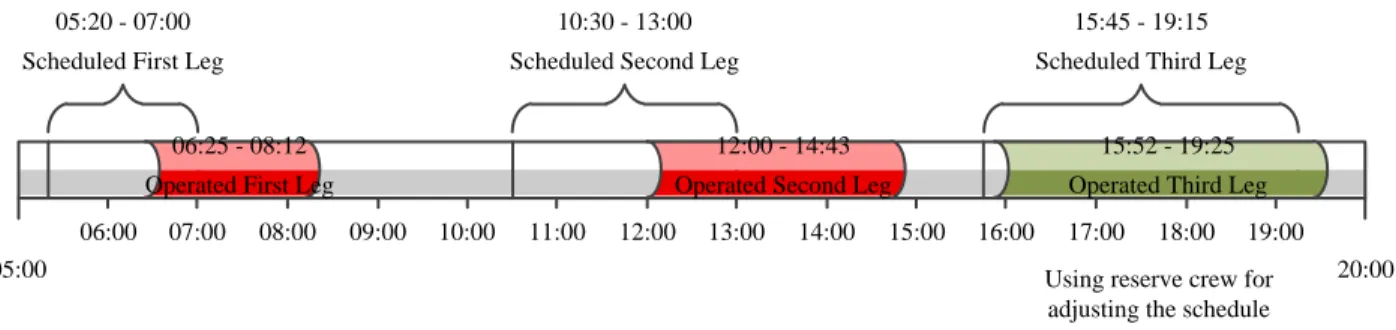
Figure 3-2: Change of scheduled pairing due to a flight delay. First two legs of the pairing were operated by delay and for adjusting the schedule pilot of the third leg was operated by a reserve

pilot.

Figure 3-2 and Table 3.1 describe a possible example of changes in schedule because of delay. The pairing is planned for 3 legs. It starts from city A and passes cities B and C and ends in the base of the pairing, City A. The awarded captain for this pairing is ID0015. In the operations, the first two legs of the pairing have been operated with delays. As the second leg arrived later than scheduled (it arrived at 14:43 instead of 13:00, see Arrival time column of Table 3.1), pilots did not have enough resting time between the second and third legs. In this case operations manager had to decide either to operate the third leg with a delay or to change the flight crew. The decision was to change the crew because the crew status, in the second part of Table 3.1, for third leg is deadhead and it is different from the scheduled crew status. Reserve crews operated the last leg of the pairing and the scheduled crew were in the flight as deadhead pilots for coming back to their base. The details and changes are shown with red font in Table 3.1.

Table 3.1: An example of change of scheduled pairing due to a flight delay.

05:00 20:00

06:00 07:00 08:00 09:00 10:00 11:00 12:00 13:00 14:00 15:00 16:00 17:00 18:00 19:00 05:20 - 07:00

Scheduled First Leg

10:30 - 13:00 Scheduled Second Leg

15:45 - 19:15 Scheduled Third Leg 06:25 - 08:12

Operated First Leg

15:52 - 19:25 Operated Third Leg 12:00 - 14:43

Operated Second Leg

Using reserve crew for adjusting the schedule

Flight

Number Departure Arrival

Captain ID Departure Date Departure time Arrival Date Arrival time Duration Crew Status 110 A B ID0015 29/09/2013 5:20 29/09/2013 7:00 100 pilot 240 B C ID0015 29/09/2013 10:30 29/09/2013 13:00 150 pilot 375 C A ID0015 29/09/2013 15:45 29/09/2013 19:15 210 pilot Flight

Captain ID Departure Date Departure time Arrival Date Arrival time Duration Crew Status 110 A B ID0015 29/09/2013 6:25 29/09/2013 8:12 107 pilot 1420 B C ID0015 29/09/2013 12:00 29/09/2013 14:43 163 pilot 375 C A ID0015 29/09/2013 15:52 29/09/2013 19:25 213 deadhead Schedule Operations Records Column in GREEN fills after bidding process

(38)

Figure 3-3: Change of scheduled pairing because of sickness. The block holder captain called sick, as there has not been reserve pilot in the pairing base, a reserve pilot has been transferred to

the base of the pairing.

Another example of schedule change is shown in Figure 3-3 and Table 3.2. In this case, the block holder captain (ID0224) called sick before the pairing. Therefore, the same rows of the schedule for this pairing (part 1 of Table 3.2) have been created in the operations’ record table (part 2 of Table 3.2). The only difference is in the crew status column which indicates calling sick happened during operations. The pairing was based in city Y and there were no appropriate reserve captain in that city and the operations manager moved a reserve (ID0754) from another city (X) as deadhead to operate this pairing. At the end of the pairing, the reserve captain returns to his base as deadhead. In Table 3.2 the details of this scenario is illustrated.

Table 3.2 : An example of change in scheduled pairing because of sickness.

7:00 AM 8:00 PM

09:30 - 10:40 Deadhead

13:05 - 20:27 Operated First Leg

08:00 - 15:23 Operated Second Leg

18:45 - 19:55 Deadhead 13:00 - 20:10

Scheduled First Leg

08:00 - 15:20 Schedule Second Leg 08:00

Calling Sick

Flight

Captain ID Departure Date Departure time Arrival Date Arrival time Duration Crew Status 857 Y Z ID0224 29/09/2013 13:00 29/09/2013 20:10 430 pilot 444 Z Y ID0224 30/09/2013 8:00 30/09/2013 15:20 440 pilot Flight

Captain ID Departure Date Departure time Arrival Date Arrival time Duration Crew Status 857 Y Z ID0224 29/09/2013 13:00 29/09/2013 20:10 430 sick 444 Z Y ID0224 30/09/2013 8:00 30/09/2013 15:20 440 sick Flight

Captain ID Departure Date Departure time Arrival Date Arrival time Duration Crew Status 105 X Y ID0754 29/09/2013 9:30 29/09/2013 10:40 70 deadhead 857 Y Z ID0754 29/09/2013 13:05 29/09/2013 20:27 442 replaced 444 Z Y ID0754 30/09/2013 8:00 30/09/2013 15:23 443 replaced 248 Y X ID0754 30/09/2013 18:45 30/09/2013 19:55 70 deadhead Schedule

Column in GREEN fills after bidding process

Operations Records

(39)

3.2.3 Operations’ Record Table

The records of operations are published in a table called operations’ record. Let 𝕆_𝑖𝑗 denotes the operations’ record for position i and month j. When some uncontrolled and unpredicted events happen during the operations and the scheduled pairing breaks, the operations managers and their systems consider the problem flight-wise rather than pairing-wise as in the planning phase. This is the reason that in the operations’ record table, each record of this table is a flight, and flights must be considered as individuals.

The only information used from the operations’ record table in this study is the sickness indicator. As the predictions must be based on the scheduled pairings, all the other attributes that are used in modeling and predicting comes from schedule tables 𝕊_𝑖𝑗. That means, in this study, sickness in a flight is equal to scheduled flight duration if the corresponding planned pilot is reported sick in the operations’ record table. For example in the explained case of Table 3.2, time of sickness is considered 430 minutes and 440 minutes for the first leg and for the second leg, respectively. The same as flight scheduled duration (ninth column of the first part of Table 3.2) and not their actual and operated duration (ninth column of the third part of Table 3.2).

3.3 Pairing Characteristics and attributes

In airline industry, pilots bid on the pairings and based on the honouring seniority, it is possible to have some undesired pairings for some pilots in a monthly work-schedule. Therefore we may expect that pairing characteristics have a big effect on their choices. Some pairings are for 4 or 5 consecutive days and some others are for just one day. Some of them contain a lot of deadhead credit and some happen during the weekend and holidays. As there is no available information about the pilots’ preferences in this study, we consider pairing characteristics as the only covariates of the model to extract their hidden information during the analysis. A list of these attributes and a brief explanation for each of them is presented in Table 3.3.

(40)

Table 3.3: List of the attributes

Row Attribute Attribute Name Description Type of

Attribute

1 UC Unique Code Distinguish uniquely each pairing

for one pilot. ID

2 BP Bid period Pairing block month. ID

3 P Position Scheduled position of the pairing. ID

4 LN Leg Numbers Number of legs in a pairing. Integer

5 TC Total Credit Total flight minutes during a

pairing. Numeric

6 NC Night Credit Night flight minutes during a

pairing. Numeric

7 DC Day Credit Day flight minutes during a pairing. Numeric 8 DH Deadhead Credit Flight minutes credited to a pilot to

be deadhead during a pairing. Numeric 9 R Return to base Number of legs in a pairing with the

same departure as the base. Integer

10 TT Total time

Total time of the pairing from departure time of first leg to arrival

time of the last leg.

Numeric

11 B Base Base of the pairing, departure city

of the first leg. Nominal 12 AS Actual Seat The role of the pilot in the flight. Nominal 13 WT Weekend Time Percentage of the pairing's total

time that passes during weekend. Proportion

14 M Month Month of the year that pairing

belongs to. Date

15 SH Start Hour Hour of day in which pairing starts Nominal 16 EH End Hour Hour of day in which pairing ends Nominal 17 SD Start Day Week day in which pairing starts Nominal

18 ED End Day Week day in which pairing ends Nominal

19 W Week Week of the year that pairing

belongs to Nominal

20 s Scheduled flying

time for sick pilot

Total credit of the pairing in which

pilot was sick. Numeric

(41)

CHAPTER 4 METHODOLOGY

In this chapter we represent the proposed methodology for predicting sickness. Data pre-processing methods are explained in Section 4.1. In Section 4.2, calculating sickness hours based on a decision tree is presented and the complexity of selecting the best level of the tree is illustrated by an example. The learning process for making a decision tree is presented in Section 4.3 and in Section 4.4 the predicting algorithm is explained.

4.1 Data pre-processing

4.1.1 Merging Tables and Data Cleaning

As explained in Section 3.2, for each position and each month we have 2 tables, pairing schedule, 𝕊_𝑖𝑗, and operations’ record, 𝕆_𝑖𝑗. The pairing characteristics, which were defined as the variables in the model, are in the pairing schedule table and the sickness indicator is a variable of operations’ record table. Hence, we need to merge these two tables for adding sick information to the schedule table.

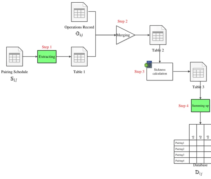
The steps of the merging process are shown in Figure 4-1. The pairing schedule table is a pairing-wise table and the operations’ record table is a flight-pairing-wise table so, for merging these two tables we first need to match the individual of these tables. In the first step, the pairing schedule table, 𝕊_𝑖𝑗, is extracted to its flight legs and we obtain Table 1, which is a flight-wise schedule table. In the second step, we merge Table 1 and the operations’ record table flight by flight and obtain Table 2. In the third step, sickness calculation sub-process is applied to Table 2 for adding flight sick minutes, the scheduled flying minutes with a pilot reported as sick. The result is Table 3 which is used in step 4 for the summing-up sub-process. At the last step, the table will be summarized so that each individual of the table is a pairing and each attribute is a pairing characteristic. The final table is our main database and is denoted by 𝔻_𝑖𝑗.

The reason for merging is adding a sick indicator to the pairings schedule. We remove all other operational information of the table as a data cleaning step to improve the speed of running statistical codes later on. Afterwards, the sickness for each flight will be calculated based on this database. In the next section we explain the sickness calculation step.

(42)

Figure 4-1: Data pre-processing steps. Step 1 is extracting pairing schedule table to its flights. Step 2 is merging obtained table with operations’ record table. In step 3, sickness calculation applies to Table 2 and its result is Table 3. Finally by summing up for each variable in Table 3

over each pairing we obtain the final table.

4.1.2 Sickness Calculation and Sick Attributes

We show flight related attributes with upper-case letters and pairing related attributes with lower-case letters, i.e. 𝐶 denotes total credit of a flight while 𝑐 denotes the total credit of a pairing. Suppose that 𝕊_𝑖𝑗 has 𝐾_𝑖𝑗 pairings 1,2, … , 𝐾_𝑖𝑗 and pairing k has 𝐿_𝑘 legs 1,2, … , 𝐿_𝑘. After adding the sick indicator, 𝐼𝑖𝑗𝑘𝑙, to the schedule pairings table, flight sick minutes, 𝑆𝑖𝑗𝑘𝑙, equals to the schedule

total credit of the flight (𝐶𝑖𝑗𝑘𝑙) if the pilot in the flight was reported as sick and 0 otherwise, i.e.

Pairing2 v1 v2 v3 Pairing1 Pairing3 Pairing4 Database Extracting Pairing Schedule Pairing Schedule Table 3 Table 3 Table 2 Table 2 Operations Record Operations Record Table 1 Table 1 Summing up Sickness calculation Step 1 Step 2 Step 3 Step 4 Merging

(43)

𝑆_{𝑖𝑗𝑘𝑙} = {𝐶𝑖𝑗𝑘𝑙, if 𝐼𝑖𝑗𝑘𝑙 is true

0, otherwise. (4-1)

Sick minutes for a pairing is equal to the sum of flight sick minutes, 𝑆𝑖𝑗𝑘𝑙, over all its legs. Hereafter

𝑠𝑖𝑗𝑘 indicates the sum of the flying minutes that have been planned for a pilot during pairing k of

pairings schedule table for month j and position i

𝑠𝑖𝑗𝑘 = ∑ 𝑆𝑖𝑗𝑘𝑙 𝐿𝑘

𝑙=1

. (4-2)

And finally the total sickness in month 𝑗 for position i is the sum of pairing sickness over all its pairings

𝑠_𝑖𝑗 = ∑ 𝑠_𝑖𝑗𝑘

𝐾𝑖𝑗

𝑘=1

. (4-3)

4.2 Decision tree and its levels

In every data mining study, it is necessary to visualize data and provide some descriptive statistics for having a general idea about the structure of the data. Sometimes visual representation of the data helps a lot in understanding the important information in the data or leads to the appropriate method of analyse. We first started working on these statistics to get familiar with the data, some of the most important and useful data visualization techniques, which we used in this study, are proposed later in Section 5.1.

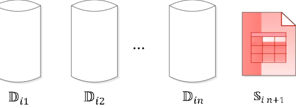
As it has been explained in the previous section, we have two main databases for predicting new month sickness. Let n merged tables be available for position i, 𝔻𝑖1, 𝔻𝑖2, … , 𝔻𝑖𝑛. After publishing

new month pairing schedule (𝕊_{𝑖 𝑛+1}), a suitable method for prediction must be able to predict total sickness hours for this new month (𝑠𝑖 𝑛+1).

(44)

Figure 4-2: Available datasets for predicting new month sickness. All the previous databases (𝔻_𝑖1, 𝔻_𝑖2, … , 𝔻_𝑖𝑛) and the schedule of new month, (𝕊_{𝑖 𝑛+1}), can be used in prediction. In each of the datasets 𝔻_𝑖1, 𝔻_𝑖2, … , 𝔻_𝑖𝑛, the response variable is defined as the sick indicator. This variable is denoted by 𝑦𝑖𝑗𝑘 which indicates the sickness in pairing k of position i during month j

and is a binary variable.

𝑦_𝑖𝑗𝑘 = {1, if 𝑠𝑖𝑗𝑘 > 0

0, otherwise (4-4)

Let 𝔗 be the complete decision tree obtained by using all the datasets 𝔻_𝑖1, 𝔻_𝑖2, … , 𝔻_𝑖𝑛, where the sick indicator is the response variable and the pairing characteristics (Table 3.3) are the explanatory variables. If 𝔗 has m terminal nodes which represent m regions on the space of pairing characteristics as 𝓇₁, 𝓇₂, … , 𝓇_𝑚 and the assigned probability of sickness in each region is 𝓅₁, 𝓅₂, . . , 𝓅_𝑚; then the estimation of sickness for the new month can be calculated as

𝑠̂(𝔗, 𝕊𝑖 𝑛+1) = ∑ 𝓅𝑘𝑐𝑘 𝑚 𝑘=1

, (4-5)

where 𝑐_𝑘is the sum of total credits in k th region of the pairing schedule of the new month.

This is our proposition for estimating the monthly sickness based on a decision tree and a published pairing schedule. Like any other decision tree, a question arises: how deep must the decision tree be or at which level the decision tree must be pruned?