Sequential estimation of surface water mass changes from daily satellite gravimetry data

Any correspondence concerning this service should be sent

to the repository administrator:

tech-oatao@listes-diff.inp-toulouse.fr

This is an author’s version published in:

http://oatao.univ-toulouse.fr/22600

Official URL

DOI :

https://doi.org/10.1007/s00190-014-0772-2

Open Archive Toulouse Archive Ouverte

OATAO is an open access repository that collects the work of Toulouse

researchers and makes it freely available over the web where possible

To cite this version:

Ramillien, Guillaume and Frappart, Frank

and Gratton, Serge and Vasseur, Xavier Sequential estimation of

surface water mass changes from daily satellite gravimetry data.

(2015) Journal of Geodesy, 89 (3). 259-282. ISSN 0949-7714

DOI 10.1007/s00190-014-0772-2

Sequential

estimation of surface water mass changes

from

daily satellite gravimetry data

G. L. Ramillien · F. Frappart · S. Gratton · X. Vasseur

Abstract We propose a recursive Kalman filtering approach to map regional spatio-temporal variations of ter-restrial water mass over large continental areas, such as South America. Instead of correcting hydrology model outputs by the GRACE observations using a Kalman filter estimation strategy, regional 2-by-2 degree water mass solutions are con-structed by integration of daily potential differences deduced from GRACE K-band range rate (KBRR) measurements. Recovery of regional water mass anomaly averages obtained by accumulation of information of daily noise-free simu-lated GRACE data shows that convergence is relatively fast and yields accurate solutions. In the case of cumulating real GRACE KBRR data contaminated by observational noise, the sequential method of step-by-step integration provides estimates of water mass variation for the period 2004–2011 by considering a set of suitable a priori error uncertainty parameters to stabilize the inversion. Spatial and temporal averages of the Kalman filter solutions over river basin sur-faces are consistent with the ones computed using global

G. L. Ramillien

Centre National de la Recherche Scientifique (CNRS), 3 Rue Michel-Ange, 75016 Paris, France

F. Frappart

Université Paul Sabatier (UPS), Toulouse, France G. L. Ramillien (

B

Groupe de Recherche en Géodésie Spatiale (GRGS), GET UMR5563-Observatoire Midi-Pyrénées,

14, Avenue Edouard Belin, 31400 Toulouse Cedex 01, France e-mail: Guillaume.Ramillien@get.obs-mip.fr

S. Gratton

ENSEEIHT-IRIT, Toulouse, France S. Gratton · X. Vasseur

CERFACS, Toulouse, France

monthly/10-day GRACE solutions from official providers CSR, GFZ and JPL. They are also highly correlated to in situ records of river discharges (70–95 %), especially for the Obidos station where the total outflow of the Amazon River is measured. The sparse daily coverage of the GRACE satellite tracks limits the time resolution of the regional Kalman filter solutions, and thus the detection of short-term hydrological events.

Keywords GRACE satellite gravimetry · Continental hydrology · Kalman filtering · Regional solutions

1 Introduction

Launched in March 2002, the Gravity Recovery and Climate Experiment (GRACE) mission has globally mapped the tem-poral variations of the Earth’s gravity field at an unprece-dented millimetre precision in terms of geoid height thanks to the accurate inter-satellite measurements made by the on-board K-band range (KBR) system (Tapley et al. 2004), and by now for more than 12 years. Pre-processing of Level-1 GRACE data consists of removing the effects of known a priori gravitational accelerations such as static gravity field, atmosphere and ocean mass changes, pole and oceanic tides from the measurements to produce Level-2 solutions that consist of “reduced” Stokes coefficients (i.e., dimensionless spherical harmonic coefficients of the geopotential—see the-oretical aspects in Hofmann-Wellenhof and Moritz 2006) up to degree 90, or equivalently, of spatial resolutions of 200–300 km (Bettadpur 2007; Fletchner 2007; Chambers and Bonin 2012; Dahle et al. 2012). These global Level-2 solutions correspond to the gravity signatures of not mod-elled surface mass variations such as sudden earthquakes and continuous glacier melting, but mainly water mass transport

for detecting more localized hydrological events lasting a few days.

Previously, Kurtenbach et al. (2009,2012) andSabaka et al.(2010) have proposed a recursive Kalman filter scheme for estimating daily Level-1B GRACE data taking into account statistical information on process dynamics and noise from geophysical models to gain in temporal resolution. Kurten-bach et al.(2009) have applied a Kalman filtering after hav-ing removed annual and semi-annual parts to obtain gravity variation time series of Stokes coefficients at daily intervals. These corrections have enabled them to consider a stationary isotropic process noise in time and space to derive an expo-nential covariance function of a first-order Markov process. In describing this process noise, Kurtenbach et al. (2009) have used a priori time and space covariances on Stokes coef-ficients. Unfortunately, daily spherical harmonics solutions remain smooth in space, due to the poor geographical cover-age of the daily satellite tracks.

In this article, no a priori model is corrected by the GRACE observations, but the estimate is built iteratively by cumulat-ing information of daily GRACE satellite tracks. As there are no daily GRACE satellite data to cover the surface of the Earth efficiently, we demonstrate that estimating regional time-cumulated solutions by the successive injection of daily GRACE tracks is achievable. The progressive integration of satellite observations has the advantage of avoiding inver-sion of large systems of equations in the determination of time-constant maps of water mass variation. The sequential method we propose is inspired from previous methods. How-ever, our Kalman filter estimation is applied to regional solu-tions instead of global Stokes coefficients. First, the method-ology of the two stages of the Kalman filter estimation (i.e., projection and correction) is presented, and secondly, its application for inverting simulated GRACE satellite data is shown. Thirdly, both the analysis of the convergence and the detection of short-term events are made by noise-free simula-tions from hydrology model outputs. This method is applied to invert along-track potential anomalies derived from real GRACE KBRR measurements to recover multi-year series of 2-by-2 degree solutions of water mass variations over South America. In the following, we use the term “regional averaged (or equivalently, cumulated) solutions computed at successive daily time steps”, but this does not imply a daily time resolution. Then, these estimates are confronted to the official global monthly GRACE solutions provided by CSR, GFZ and JPL (Release 5) filtered using the indepen-dent component analysis approach (Frappart et al. 2011), and 10-day regional solutions fromRamillien et al.(2012), 10-day global solutions from GRGS (Bruinsma et al. 2010), and GLDAS-NOAH (Rodell et al. 2004) and WGHM (Hunger and Döll 2008) outputs, as well as rapid events described by river discharge observations for validation. The possi-bility of detecting short-term water mass events is finally over continental areas. North–south striping is particularly

visible in the tropics where coverage of satellite tracks is poor due to (1) sparse GRACE track sampling in the lat-itudinal direction, (2) propagation of errors of the a priori correcting model accelerations (Han et al. 2004; Thompson et al. 2004; Ray and Luthcke 2006) and (3) numerical corre-lations generated while solving the undetermined systems of equations for high-degree Stokes coefficients (Swenson and Wahr 2006).

Short-term mass variability with periods from hours to days of ocean tides and atmosphere is removed using de-aliasing techniques of correcting model outputs. While the atmosphere pressure fields from ECMWF allow a reason-able de-aliasing of high frequency caused by non-tidal atmospheric mass changes, errors due to tide model appear in the GRACE solutions, especially from diurnal (S1) and semi-diurnal (S2) tides (Han et al. 2004; Ray and Luthcke 2006;

Forootan et al. 2014). Thompson et al. (2004) showed that

the degree error increased by a factor ∼20 due to atmospheric aliasing, ∼10 due to ocean model and ∼3 due to continental hydrology, e.g., aliasing of the S2 tide has a strong impact on the determination of the C20 spherical harmonic coefficient

of the geopotential (Seo et al. 2008). See, e.g., Guo et al.

(2010) to know about the reduction of atmosphere aliasing

by Gaussian smoothing.

A regional approach alternative to the classical global one has been more recently proposed to improve geograph-ical localization of patterns of water storage change. This energy integral method consists of recovering equivalent-water thicknesses of juxtaposed 2-degree tiles from GRACE inter-satellite velocity residuals, by considering matrix reg-ularization techniques for solving ill-posed problems, but without using spherical harmonics for representing water mass variations (see Ramillien et al. 2011, 2012). These

multi-year series of 10-day regional solutions are compa-rable to independent datasets, such as local water level in the Amazon Basin, and thus they provide realistic amplitudes of water mass change from seasonal to inter-annual timescales over South America.

So far, global and regional solutions have been produced as weekly, 10-day and monthly averages from GRACE data, leading to a loss of resolution in time. In other words, global or regional averaging suppresses events with a gravity sig-nature of a few days and thus does not enable us to capture them. Moreover, determining the regional equivalent-water heights for each separate time interval would neglect the temporal correlation between successive independent inter-vals imparted by the temporal dynamics of the water mass processes. While regional solutions computed as averages on constant 10-day intervals proved to be realistic snap-shots of the surface water mass variability (Frappart et al. 2013a, b; Seoane et al. 2013), the next challenge is to attempt

discussed and tested by simulating localized water mass anomalies.

2 Datasets

2.1 Independent hydrological datasets

2.1.1 WGHM land water storage

The WaterGAP Global Hydrology model (WGHM) (Döll et al. 2003;Hunger and Döll 2008) is a conceptual model that simulates the water balance on continental areas at a spatial resolution of 0.5◦. It describes the continental water cycle using several water storage compartments that include interception, soil water, snow, groundwater and surface water (rivers, lakes and wetlands). We consider the sum of all these contributions and called it Total Water Storage (TWS) to be comparable to GRACE observations, as these latter data correspond to the integrated continental hydrology change without distinguishing each compartment. WGHM has been widely used to analyse spatio-temporal variations of water storage globally and for large river basins (Günter et al. 2007). In this study, we use daily TWS grids from the model version WGHM 2.1f described byHunger and Döll(2008) to simu-late the GRACE hydrology-resimu-lated geopotential anomalies, and recover the starting TWS variation grids, as accurately as possible from these modelled geopotential anomaly tracks over a region, to demonstrate the feasibility of the Kalman filter approach for estimating TWS change from GRACE observations.

2.1.2 GLDAS NOAH land water storage

The NOAH (NCEP, OSU, Air Force and Office of Hydrol-ogy) land surface model (LSM) simulates surface energy and water fluxes/budgets (including soil moisture) in response to near-surface atmospheric forcing and depending on sur-face conditions (e.g., vegetation state, soil texture and slope) (Ek et al. 2003). The data used in this study are soil mois-ture (SM) storage values from the NOAH LSM, with the NOAH simulations being driven (parameterization and forc-ing) by the Global Land Data Assimilation System (GLDAS) (Rodell et al. 2004). These SM estimates from GLDAS-NOAH version 2 have a spatial resolution of 1◦and a tem-poral resolution of 3 h. They are accessible via the Hydrol-ogy Data Holdings page at the Goddard Earth Sciences Data and Information Services Center, http://disc.sci.gsfc.nasa. gov/hydrology/data-holdings. They were cumulated on the four soil layers representative of the top 2 m of the soil from the GLDAS-NOAH model and resampled at a daily timescale over the time period 2003–2010.

2.1.3 Measurements of river discharge

Time series of daily water discharges from in situ gauges located in Obidos (Amazon), Ciudad Bolivar (Orinoco), Tucurui (Tocantins), and Chapeton (La Plata) are used for comparisons to daily, 10-day and monthly anomalies of GRACE-based TWS over 2003–2010. These in situ records were downloaded for the period 2003–2010 from: (1) the Venezuelian water agency (Instituto Nacional de Meteorologia e Hidrologia—INAMEH) for Ciudad Bolivar (63◦36′29′′W; 8◦26′20′′N); (2) the hydrological information system Hidroweb (http://hidroweb.ana.gov.br/) of the Brazil-ian water agency (Agência Nacional de Aguas—ANA) for Obidos (55◦39′25′′W; 1◦55′23′′S), Manacapuru (60◦36′32′′ W; 3◦18′58′′S), Fazenda Vista Alegre (60◦01′34′′W; 4◦53′ 53′′_{S), Porto Velho (63}◦₅₆′₄₆′′_{W; 8}◦₄₇′₅₉′′_{S) and Tucurui}

(49◦40′59′′W; 3◦46′59′′S) gauges; and (3) the Argentinian water agency (Instituto Nacional del Agua—INA) through the online database Base de Datos Hidrológica Integrada (BDHI—http://www.hidricosargentina.gov.ar/) for the Chapeton station (60◦16′59′′W; 31◦34′26′′S).

2.1.4 Global GRACE solutions

Three processing centres including the Center for Space Research (CSR), Austin, Texas, USA, the GeoForschungs-Zentrum (GFZ), Potsdam, Germany and the Jet Propulsion Laboratory (JPL), Pasadena, California, USA, and forming the Science Data Center (SDC) are in charge of the processing of the GRACE data and the production of Level-1 and Level-2 products. These products are distributed by the GFZ’s Inte-grated System Data Center (ISDC—http://isdc.gfz-potsdam. de) and the JPL’s Physical Oceanography Distributive Active Data Center (PODAAC—http://podaac-www.jpl.nasa.gov). Pre-processing of Level-1 GRACE data (i.e., positions and velocities measured by GPS, accelerometer data and KBR inter-satellite measurements) is routinely made by the SDC, as well as monthly global GRACE gravity solutions (Level-2). These latter solutions consist of time series of monthly averages of Stokes coefficients (i.e., dimensionless spher-ical harmonics coefficients of geopotential) developed up to a degree between 50 and 120 that are adjusted from along-track GRACE measurements. A dynamical approach, based on the Newtonian formulation of the satellite’s equa-tion of moequa-tion in an inertial reference frame, centred at the Earth’s centre of mass combined with a dedicated modeling of the gravitational and non-conservative forces acting on the spacecraft, is used to compute the monthly GRACE solu-tions. During the estimation process, atmospheric and ocean barometric redistribution of mass variations are removed from the GRACE coefficients using ECMWF and NCEP reanalysis for atmospheric mass variations and ocean tides, as well as global ocean circulation models (Bettadpur 2007;

Fletchner 2007). The GRACE coefficients are hence residu-als that should include continental water storage change, and also signals from other geophysical phenomena and errors from correcting models and noise. The monthly GRACE solutions differ from one official provider to another due to the differences in the data processing, the choice of the correcting models and the data selection for computing the monthly averages.

A post-processing method based on independent com-ponent analysis (ICA) was applied to the Level-2 GRACE solutions from different official providers (i.e., CSR, GFZ, JPL), after a 400-km Gaussian pre-filtering. The separa-tion is based on the assumpsepara-tion of statistical independence between the sources that compose the measured signals. The estimated contributors to the observed gravity field are forced not to be correlated numerically by imposing diagonal cross-correlations. The efficiency of ICA for separating land hydrology-related signals from noise by combining Level-2 GRACE solutions has previously been demonstrated in

Frappart et al.(2010, 2011).

The GRGS-EIGEN GL04 models are derived from Level-1 KBRR measurements and LAGEOS Level-1 and 2 data for enhancement of lower harmonic degrees and using an empiri-cal stabilization; thus, these solutions do not require any low-pass filtering to get rid of striping (Lemoine et al. 2007; Bru-insma et al. 2010). Corresponding 10-day and monthly grids of TWS for the period 2003–2010 are available at:http:// grgs.obs-mip.fr.

2.2 GRACE-based residual potential differences to be inverted

degree and order 160; (2) 3D body perturbations DE403 of Sun, Moon and six planets (Standish et al. 1995); (3) solid Earth tides of the IERS conventions 2003 (McCarthy and Petit 2003); (4) solid Earth pole tide of the IERS conven-tions; (5) oceanic tides FES2004 to degree and order 100 (LeProvost et al. 1994); (6) Desai model of the oceanic pole tide (Desai 2002); (7) atmospheric pressure model ECMWF 3D grids per 6 h; and (8) oceanic response model MOG2D (Carrère and Lyard 2003). These KBR Rate (KBRR) resid-uals represent the gravitational effects of non-modelled phe-nomena, and mainly the contribution of continental hydrol-ogy. They are easily converted into variations of along-track potential differences between the two GRACE satellites, fol-lowing the energy integral method as proposed earlier by

Jekeli(1999),Han et al.(2006) and latelyRamillien et al.

(2011). Once corrected from known gravitational accelera-tions, along-track Residual Differences of Potential (RDP) mainly caused by hydrology variations in a selected conti-nental region can reach ±0.1 m2/s2 within a precision of ∼10−3m2/s2 (seeRamillien et al. 2011). These form the initial data set for our Kalman filter approach.

3 Methodology

3.1 The forward problem

We suppose that the continental region consists of M juxta-posed surface elements ( j = 1, . . . , M) of area Sj located

at longitude λj and latitude θj, and characterized by an

equivalent-water height hj. The grid steps in longitude and

latitude are 1λ and 1θ respectively, in the case of a geo-graphical grid. Let Ŵk be the N -by-M Newtonian matrix

that relates the equivalent uniform water height hj and the

GRACE-based potential differences Yi (i = 1, . . . , N ) for

each daily period of observation k. The coefficients of this matrix are simply deduced from the inverses of the Carte-sian distances ξ between the surface element heights Xkand

the successive positions of the GRACE satellites flying over the considered region (seeRamillien et al. 2011). Then, the observation equation can be written as:

ŴkXk =Yk+vk (1)

where vkis a zero-mean process noise usually drawn from a

zero-mean multivariate normal distribution with covariance matrix Rk (i.e., vk ∼ N (0; Rk)). In the construction of the

Newtonian matrix Ŵk, developing the inverse of the distance

in sums of Legendre polynomials of n = 300−500 terms enables us to introduce the elastic Love numbers kn, to take

compensation of surface water masses by elastic response of the Earth’s surface into account (Ramillien et al. 2011).

Additional information has to be included to find a stable mass variation estimate. In this study, we use a simple first-The K-band range (KBR) is the key science instrument of

GRACE which measures the dual one-way range change of the baseline between the two coplanar, low-altitude satellites, with a precision of ∼0.1 µm/s on velocity difference, or equivalently, 10 µm in terms of line-of-sight (LOS) distance after integration versus time (Bruinsma et al. 2010). The aver-age distance between the two GRACE vehicles is ∼220 km. The Level-1B KBR data represent the more precise measure of gravity variations sensed by the GRACE satellite tandem with a 10−7 _{m/s accuracy, that gives access to surface water}

mass transfers. Coupled with the accurate 3-axis accelerom-eters measuring the effects of non-conservative forces acting on the satellites (i.e., atmospheric drag and solar pressure) and a priori models for correcting atmosphere and ocean mass, oceanic and solid tides and polar tides, KBR rate resid-uals are computed by least-squares dynamical orbit determi-nation of 1-day-long and 5-second sampled tracks. A pri-ori gravitational force models for numerical orbit integration of the GRACE satellites A and B prepared at the GRGS centre in Toulouse (Bruinsma et al. 2010) are: (1) a static gravity field model EIGEN-GRGS.RL02.MEAN-FIELD to

order Gauss–Markov process to model the evolution of the current estimate Xk with time. More precisely, given k > 1,

we use the simple prediction equation:

Xk=Xk−1+wk (2)

where wkis a zero-mean process noise usually drawn from a

zero-mean multivariate normal distribution with covariance matrix Qk (i.e., wk ∼ N (0; Qk))describing the errors of

the process. Although this dynamic is known to remain very crude, promising results will be shown in Sect.4. The authors are well aware of the fact that this model can be improved by introducing an evolution model that might consist in exploiting outputs of hydrology models such as WGHM and GLDAS. FollowingKurtenbach et al.(2009), a more sophis-ticated dynamical equation than Eq.2has been considered through a linearized dynamic (i.e., a finite difference matrix obtained from WGHM) that is described by the prediction equation (Eq. 2). Unfortunately, the results were not sig-nificantly different from the ones shown in Sects.5and6. These disappointing results may be due to the use of a lin-earization technique or to the presence in the observations of effects not taken into account by the model. As the New-tonian operator Ŵk constructed from the relative Cartesian

distances and applied to the unknown parameters (i.e., the equivalent-water heights) is completely linear (see Ramil-lien et al. 2011,2012), for a given set of a priori uncertainty parameters, the Kalman filter estimate considering the entire GRACE-based RDP dataset is the same as the one obtained by summing all the separate Kalman filter estimates. This is the case if the complete RDP series are decomposed into pure dominant annual and semi-annual components plus any kind of RDP sub-dataset. In particular, the problem of recovering short-term hydrological events by tuning a priori uncertainty parameters is tackled in Sect.6by several simulations. 3.2 The inverse problem: sequential estimation—the

Kalman filter equations

The observation equation (Eq.1) and the prediction equation (Eq.2) directly fit into the Kalman filter equation settings. The Kalman filter is a recursive estimator where one needs the knowledge of the previous state and new measurements to determine the actual state (Kalman 1960;Kalman and Bucy 1961;Evensen 2007). In our setting at iteration number k, the state of the estimator is represented by two variables: the current estimate Xk(i.e., the vector containing the

equivalent-water heights) and its error covariance matrix Pk (i.e., the

matrix of the uncertainties on the estimate).

The observations of the current state are used to correct the predicted variables to obtain a more precise estimate. First, the Kalman gain matrix is computed as:

Kk =PkŴkT

!

ŴkPkŴTk +Rk

"−1

(3)

where Rkis the covariance of the measurements errors

con-sidered as independent (i.e., Rk=σd2I, where σd2is the error

variance on the RDP Yk, and I represents the identity matrix).

Secondly, the updated a posteriori state estimate is obtained as:

X_k∗=Xk+Kk[Yk−ŴkXk] (4)

and the updated a posteriori error covariance matrix of the state estimate is computed as:

P_k∗=[I − KkŴk] Pk (5)

At the end of this step, Xk+1is deduced according to Eq.2:

Xk+1 = X_k∗and the resulting covariance matrix to be used

at the next step is simply defined as:

Pk+1=Pk∗+Qk (6)

Note that for independent potential difference observations at time interval k, Qkis often chosen as the diagonal matrix:

Qk=σp2I (7)

where σ2

p is the a priori variance of process errors. The

Kalman gain appears as a measure of the relative uncertainty of the measurements and the current state estimate, and it can be “tuned” to achieve particular performance. When the gain is high, it places more weight on the observations and thus follows them more closely, whereas when it is low, the Kalman filtering follows the model prediction, smoothing noise out. In the extreme case of gain of zero, the measure-ments are completely ignored.

4 Application

4.1 Inversion of potential differences simulated from hydrology model outputs

4.1.1 Recovery of a piece-wise time-constant water mass anomaly map

First, we need to validate the proposed sequential method of estimation by recovering “static” 30-day averaged water mass anomaly maps from GRACE-type potential differences simulated using daily outputs from WGHM, over large conti-nental areas. For this purpose, regular 2-by-2 degree grids of equivalent-water heights over South America [90◦_W–30◦_W,

60◦S–20◦N] are averaged onto monthly periods from daily WGHM outputs. GRACE-type ascending and descending tracks of 5-second sampling are easily generated by the GINS software from the satellite ephemeris data and for the region of interest. Along-track potential differences are simply com-puted at each satellite position using Eq.1without noise (i.e.,

vk=0). The test consists of recovering, as precisely as

pos-sible, the static 30-day averaged water mass anomaly map by applying the Kalman filter integration (Eqs.2–7) of succes-sive synthetic daily potential differences. The first guess is assumed to contain no hydrological signals (i.e., Xk=0=0

for all elements of this vector for “cold start”), and in the case of no starting cross-error covariances between equivalent-water heights to recover, so we start with: Pk=0 = σm2I.

Then, the solution is progressively built by accumulation of information from the daily GRACE RDP tracks.

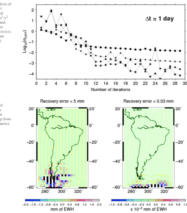
As illustrated on the top row of Fig. 1, the process of estimation converges rapidly to a stable solution, which is identical to the starting water mass anomaly after 30 days of integration. Root mean square error is typically less than 10 mm after the first iteration, 1 mm after the fifth itera-tion, 0.1 mm after the 10th iteraitera-tion, and finally 0.01 mm of equivalent-water height after a month of integration, com-pared to amplitude of ±300 mm of the hydrological pat-terns. Even short-wavelength details are revealed in the final Kalman filter solution, confirming that this noise-free recov-ery from simulated GRACE data is successful. A posteri-ori uncertainties on the fitted equivalent-water heights (i.e.,

square root of the diagonal elements of Pk)decrease,

fol-lowing the north–south direction of the tracks during the first iterations. Then they tend to be homogeneous on the whole region at the end of the fit. They are finally less than 0.1 mm, when the starting value is σm =1 mm.

Different intervals (1, 2 or 5 days) of integration yield to the same final solution in the case of recovering a noise-free 30-day constant map of water mass anomaly. Several combi-nations of σdand σmhave been tested on the simulated case

of recovery from 10−9to 10−2m2/s2, and 10 and 800 mm, respectively. A priori uncertainty on observations σdacts as

a regularization parameter and makes the inversion of the linear system for getting the Kalman gain (Eq.3) possible. Large values of this uncertainty parameter enable substantial improvements of the solution at each integration step and thus accelerate the convergence to the final estimate. On the con-trary, the convergence is slow and the final estimate is smooth when σmis low (Fig.2). In this latter case, low values of this

parameter correspond to less weight of the GRACE obser-vations in the Kalman gain K during the refreshing process of the solution. The final errors of a constant-time (monthly) map of water mass (i.e., difference between the estimate and

water heights, starting from 1 mm down to <0.05 mm (bottom row). Final absolute error is around 0.01 mm after 30 steps (i.e., 30 days) of integration. Note the residual edge effect on the Southern boundary due to geographical truncation

Fig. 1 Recovery of monthly mass variations over South America

for March 2005 from simulated along-track RDP. Units are mm of equivalent-water height. Estimated regional maps obtained by accumu-lation of 1-day data that converge to a stable solution (top row), and the decreasing of the corresponding a posteriori uncertainties on the

Fig. 2 Convergence analysis of

the recovery using a priori potential anomaly standard deviation of σd=10−9m2/s2

(i.e., exact observations) and different a priori parameter uncertainties σm: 1 mm (circles),

10 mm (triangles), 100 mm (squares), 500 mm (stars)

Fig. 3 Final error after

cumulating k = 30 days of simulated RDP data when recovering a time-constant (monthly) water mass map from daily RDP over South America for σm=1 mm (left) and

σm=500 mm (right)

the reference WGHM water mass used for simulating RDP data) remain particularly small (Fig.3), especially if σm is

large (e.g., 500 mm), suggesting that the recovery is success-ful.

4.1.2 Recovery of water mass change maps by daily updates

While the recovery of a water mass solution from RDP sim-ulated from a 30-day constant WGHM map is successful (see previous part), the next test is to estimate cumulated solutions from RDP computed using daily-varying hydrol-ogy. GRACE RDP tracks passing over South America are simulated each day at 5-second sampled orbit positions and from the WGHM (or GLDAS) total water storage (TWS) outputs for the period 2005–2007, using Eq.1without noise

(i.e, vk =0). Complete series of regional solutions of water

mass variation can be estimated by a Kalman filter inte-gration strategy on daily sampling intervals and tuning a priori error parameters. Figure4 presents regional solution when considering σd = 0.01 m2/s2 and σm = 200 mm,

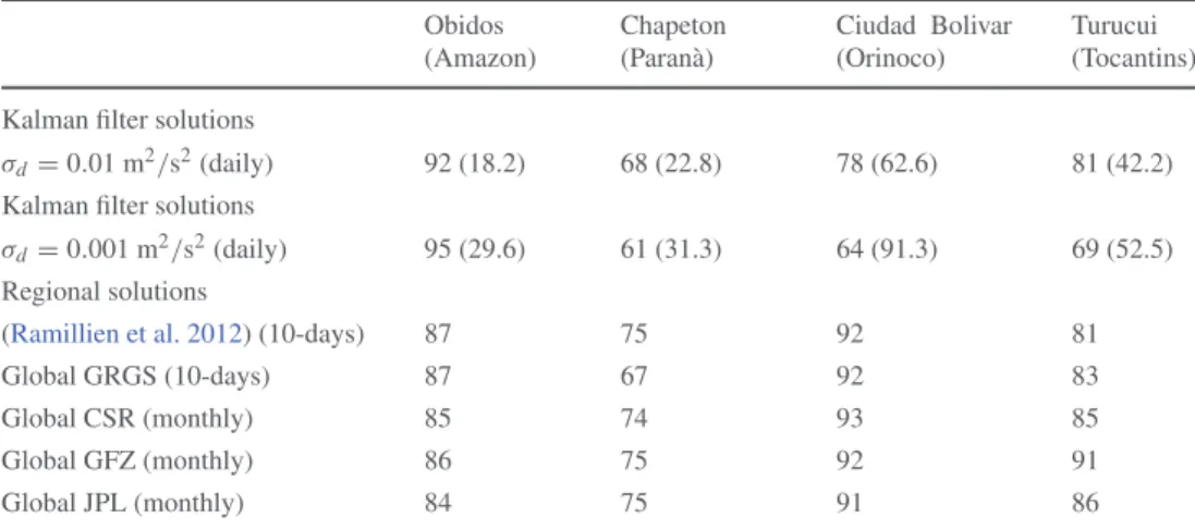
and obtained by cumulating WGHM-simulated daily along-track differences of potential. These solutions reveal realistic seasonal amplitudes in the drainage basins of South Amer-ica. Absolute errors are defined as the differences between input and recovered 2-by-2 degree water mass grids for the same day. In this case of considering very accurate RDP data (i.e., σd very small) and in the absence of additional noise,

the main hydrological structures of ±300 mm of EWH are retrieved and quite well located on the main river basins of South America.

Fig. 4 Daily 2-by-2 degree

regional maps of TWS over South America plotted at monthly intervals [units: mm of equivalent-water height (EWH)]

0.001 m2/s2 creates unrealistic meridian striping in these maps that increases with the number of days integrated into the current solution.

Tests of recovery of a “static” water mass grid, made in the previous Sect. 4.1.1, show that σm controls the

ampli-tude of information by the RDP tracks each day. In the case of recovering time-varying water mass maps with different starting values of σm, the Kalman filter process progressively

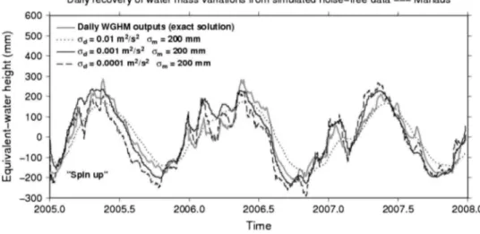
converges to the same series of daily sampling step estimates (Fig.6), and the time taken by the integration to reach this common solution (or “spin up”) from a cold start (i.e., no starting information: Xk=0 =0) is ∼3 months. This

“spin-up” is of 1 month for recovering a constant-time water mass In particular, Fig. 5 shows the water mass time series for

the surface element corresponding to Manaus (60◦

01′32′′W, 3◦₀₈′₀₆′′S), located in the centre of the Amazon basin. In

our tests for Manaus tile and using model-simulated data, a priori error uncertainty ranges from σd = 10−6 m2/s2

to σd = 0.1 m2/s2 while the parameter σm = 200 mm is

constant during the Kalman filter integration. As in the case of recovery of a time-constant map, the error of recovery of sub-monthly time-varying signals appears small when the RDP data are considered accurate (i.e., σdvery small). However,

this strong assumption permits the development of numerical instabilities. Representing the series of estimated water mass maps shows that using a priori error uncertainty σdless than

Fig. 5 Multi-year time series of

TWS for the surface tile number 357 centred over Manaus, that are obtained by integration of WGHM-simulated daily GRACE RDP data for several a priori error uncertainties, and a constant a priori error

uncertainty on the parameters to be retrieved (i.e., the

equivalent-water heights) first guess is Xk=0=0 (i.e., “cold

start”)

Fig. 6 Multi-year time series

of TWS for the surface tile number 357 (Manaus) obtained for several a priori error uncertainties on the process (i.e., σp)and the equivalent-water

heights (i.e., σm)

map, as the simulated RDP data are more consistent to each other on the period of integration and reinforce the same “sta-tic” surface distribution of water mass to be retrieved (see Sect. 4.1.1). Considering daily WGHM-based water mass variations, RDP data partly contain unexpected time-varying signals that perturb the convergence of the integration process and make the “spin up” longer. As for the a priori error σdon

the RDP observations, important values of a priori process error σp(i.e., >50 mm) generate unrealistic meridian stripes

in the estimated water mass maps.

For approaching more realistic conditions of data acquisi-tion, high-frequency random noise can be added to the model-simulated GRACE RDP, but its effect is highly amplified if considered real and accurate signals (e.g., when a ran-dom noise of 0.001 m2_/s2 _{amplitude is added in the}

sim-ulated GRACE data, the daily Kalman filter solutions are only slightly degraded but smoothed if σd =0.01 m2/s2or

∼10 % of hydrology-related RDP according toRamillien et al. 2011). Unfortunately, the recovery errors reach tens of mm when the level of noise is greater than 0.01 m2/s2. To cancel the effect of noise amplification in the inversion, we

found that the best compromise is to consider that σdand σm

are about 10−3−10−2m2/s2and 100–200 mm, respectively, with value of a priori process error σpas small as possible.

4.2 Recovery of maps from real GRACE RDP

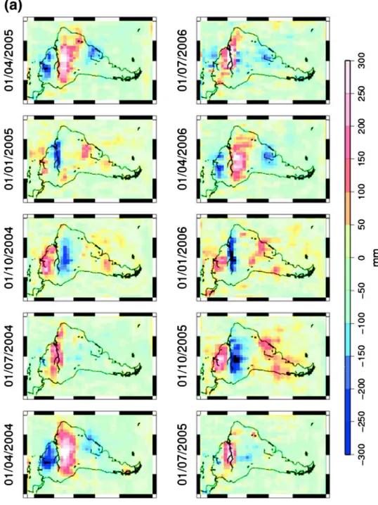
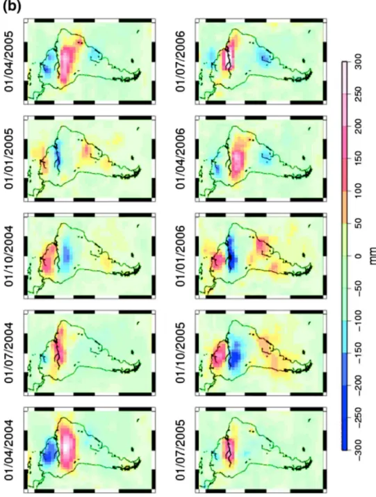
Inversion of real potential differences for continental hydrol-ogy appears complicated because of contaminating instru-mental noise, even if potential anomalies should be smooth at satellite altitude as the result of upward continuation. In return, downward continuation associated to the recovery of surface water mass anomaly amplifies the high frequencies of the signal, in particular noise of any kind. Moreover, impor-tant errors from pre-treatment such as correcting by imperfect models still remain in the orbit observations and aliased with space and time (see Sect.2.2). Another problem arises as KBR rate residuals contain unrealistic long-term variations at fractions of the satellite revolution period. The strategy lately proposed by Ramillien et al. (2011,2012) is to remove a linear trend to each potential difference track crossing the considered regions for each day before inversion, so that

a recovery of medium- and high-frequency regional water mass variations is made, but at least without adding erro-neous spatial long wavelengths. These missing wavelengths are added back from GRGS global solutions to complete the inverted signals afterwards.

2-by-2 degree water mass solutions after Kalman filter integration of daily GRACE RDP over South America for 2004–2010 are displayed on Fig. 7a, b. Starting parame-ters of Kalman filter estimation are σd =0.005 m2/s2and

σd =0.01 m2/s2Xk=0=0 (i.e., “cold start”), Pk=0=σm2I

with σm = 200 mm of equivalent-water height, and no a

priori process errors. When σd = 0.005 m2/s2, meridian

striping and edge effects rapidly dominate the Kalman filter

solutions after ∼1 year of integration of daily RDP tracks and till the end of the total period (Fig.7a). Increasing slightly this a priori parameter up to 0.01 m2/s2for an efficient regulariza-tion enables us to avoid the development of such unrealistic numerical instabilities in the time series of smoother solu-tions (Fig. 7b) where seasonal amplitudes are comparable to the ones of the global CSR solutions (Fig.7c) (see also Tables1,2). Besides, additional runs for testing different a priori errors have been made to compute multi-year series of regional Kalman filter solutions that show the seasonal alter-nating of the large water mass amplitudes in the Amazon and Orinoco river basins. Figure8illustrates the case of the time series for the surface tile centred on Manaus. It reveals

realis-Fig. 7 Snapshots of 2-by-2

degree regional solutions of TWS over South America estimated from real GRACE RDP data and assuming σm=200 mm and

σp=10 mm, and plotted at

3-month intervals revealing the dominant seasonal amplitudes of water mass over South America: Kalman filter solutions for a priori error uncertainty a σd=0.005 m2/s2

and b σd=0.01 m2/s2, and c

corresponding 400-km low-pass filtered CSR solutions (monthly averages) for the same periods for comparison

Fig. 7 continued

tic seasonal oscillations of 300–600 mm of EWH, which are clearly modulated by inter-annual variations. As expected, smooth estimates versus time are obtained when considering not precise GRACE RDP data (i.e., σd=0.1 m2/s2), but we

found that values of σdlesser than 0.007 m2/s2significantly

amplify the noise contained the real GRACE RDP. The time series of these estimated Kalman filter maps will be validated in Sect.5.

4.3 Errors due to spatio-temporal aliasing

Figure9is a visualization of the extra information brought by the GRACE satellite tracks computed as two successive

Kalman filter solutions. It shows that the Kalman filter esti-mate is daily updated in the very close neighbourhood under the satellite tracks—in a surface radius of about 600–800 km (e.g., see the numerical tests made inRamillien et al. 2012)— just under the satellite tracks where the new information is brought. While the covariance function of the RDP data is smooth at satellite altitude (∼400 km), the one of the cor-responding water mass (i.e., the source of anomaly) is also much localized on the Earth’s surface due to downward con-tinuation. This new along-track information represents a few tens of mm of EWH. Consequently, nothing is refreshed else-where, in areas which are not surveyed by the GRACE satel-lite during the considered day. This partial sampling explains

Fig. 7 continued

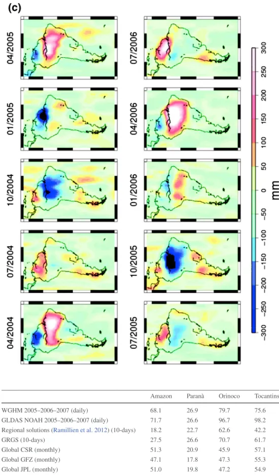
Table 1 Root mean square of

the absolute differences between daily Kalman filter solutions and different TWS datasets for spatial averages over the main drainage basins of South America [units: mm of equivalent-water height (EWH)]

Amazon Paranà Orinoco Tocantins WGHM 2005–2006–2007 (daily) 68.1 26.9 79.7 75.6 GLDAS NOAH 2005–2006–2007 (daily) 71.7 26.6 96.7 98.2 Regional solutions (Ramillien et al. 2012) (10-days) 18.2 22.7 62.6 42.2

GRGS (10-days) 27.5 26.6 70.7 61.7

Global CSR (monthly) 51.3 20.9 45.9 57.1

Global GFZ (monthly) 47.1 17.8 47.3 55.3

Table 2 Linear correlations (%)

between time series of GRACE solutions and of river discharge variations measured different stations

Root mean square (RMS) values of the differences with Kalman filter solutions are indicated between parenthesis Obidos (Amazon) Chapeton (Paranà) Ciudad Bolivar (Orinoco) Turucui (Tocantins) Kalman filter solutions

σd=0.01 m2/s2(daily) 92 (18.2) 68 (22.8) 78 (62.6) 81 (42.2)

Kalman filter solutions

σd=0.001 m2/s2(daily) 95 (29.6) 61 (31.3) 64 (91.3) 69 (52.5)

Regional solutions

(Ramillien et al. 2012) (10-days) 87 75 92 81

Global GRGS (10-days) 87 67 92 83

Global CSR (monthly) 85 74 93 85

Global GFZ (monthly) 86 75 92 91

Global JPL (monthly) 84 75 91 86

Fig. 8 Time series of TWS for

Manaus obtained by integration of real daily GRACE RDP data for several a priori error uncertainties

that the reconstruction of a “static” map takes at least 10 days of data before the Kalman integration has a sufficient spa-tial coverage of the satellite tracks at the end (see previous Sect.4.1.1). It also explains residual errors of recovery in the series of regional Kalman filter solutions, even if noise-free model-simulated RDP data are inverted (e.g., differences with model TWS values in Fig.5), since off-track small and rapid hydrological features cannot be recovered, or partly retrieved, alternatively their signatures remain in the follow-ing Kalman filter solutions. Detection of sudden and local-ized hydrological events by tuning a priori error uncertainties and considering different cases of data coverage is explored with synthetic RDP data in the discussion of Sect.6.

5 Validation of the Kalman filter solutions

Validation consists of confronting regional estimates of TWS obtained by integration of Kalman filter to existing GRACE-based products and independent datasets. For this purpose, we consider different sources of information presented in

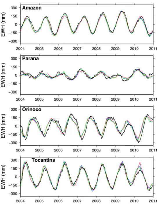
Sect. 2: daily WGHM and GLDAS land waters outputs, monthly global GRACE solutions computed by the offi-cial providers CSR, GFZ and JPL, as well as local records of river discharge. Comparisons with the 10-day regional solution of water mass variation over South America lately proposed by Ramillien et al. (2012) have been also per-formed. Global Release 5 monthly solutions from CSR, JPL and GFZ have been low-pass filtered using a classi-cal 400-km Gaussian filter (Wahr et al. 1998) and an ICA approach (Frappart et al. 2010,2011) to reduce striping. To make the sampling of Kalman filter solutions comparable with the other GRACE solutions in space and time, they have been averaged over both the 10-day and monthly inter-vals, and over the largest drainage basins of South America: Amazon (∼6 millions of km2), Paranà (∼2.6 millions of km2), Orinoco (∼1 million of km2)and Tocantins (∼0.8 million of km2_).

Statistical results of the comparisons of averages are sum-marized in Table1. It shows that the Kalman filter solutions are statistically closer to the 10-day regional solutions from

Fig. 9 Maps of the differences

between successive Kalman filter solutions and the coverage of the corresponding GRACE satellite tracks used for the daily refreshing

GLDAS-NOAH outputs at daily timescale. Significant time shifts and large differences of amplitude can be observed between GRACE-based and simulated TWS, especially on the Amazon, Orinoco and Tocantins basins. In these basins, a large part of the hydrological signal comes from slow reser-voirs as floodplains (seeFrappart et al. 2012in the case of the Amazon) and groundwater (seeChen et al. 2010in the case of the La Plata basin,Gleeson et al. 2012andFrappart et al. 2013bfor their signatures in 10-day regional solutions) that are either not or not well modelled. As a consequence, sig-nificant differences and time-lags are likely to occur between model outputs and GRACE estimates (Alkama et al. 2010) (not shown here). Larger differences in amplitude and phase Because of lower seasonal hydrological dynamics, there is

less difference for the Paranà basin (i.e., <27 mm of EWH RMS) and much difference for the Tocantins river (i.e., up to 98 mm of EWH RMS). Figure 10 shows a superposition of the monthly averages of the Kalman filter solutions and the global GRACE solutions. This proves that the Kalman fil-ter method succeeds in recovering amplitudes and phases of TWS. Indeed, they are consistent to the ones of 10-day and monthly global GRACE solutions (for instance, see Frap-part et al. 2013a, b), when they are averaged over large areas.

In the comparison, RMS differences are more important for the two hydrological models. Figure 11 presents the TWS time series of the Kalman filter solutions and of WGHM and

Fig. 10 Time series of TWS

for the largest drainage basins of South America obtained by averaging monthly CSR (blue), GFZ (red), JPL (green) and daily Kalman filter solutions (black)

are observed with GLDAS outputs, as this model (NOAH), contrary to WGHM, does not consider neither surface storage (water stored in the rivers and the floodplains) nor the routing of the surface runoff into the river network which contributes to surface storage in the downstream grid points. The con-tribution of surface storage to TWS represents 40–50 % in the Amazon basin (seeHan et al. 2009, 2010;Frappart et al. 2012;Paiva et al. 2013). So incorporation of total runoff outputs is likely to reconcile the GLDAS TWS variations to the GRACE-based amplitudes.

Comparisons were also achieved between 10-day and monthly GRACE and daily river discharges in the four largest drainage basins of South America (i.e., Amazon,

La Plata, Orinoco and Tocantins). They are presented in Fig.12 and Table 2. An overall good agreement is found between GRACE-derived TWS and river discharge varia-tions for all the basins (linear correlation greater than 70 % for the Kalman filter solutions for zero time-lag). Except in the case of Amazon basin where the values of correlation with discharge records reach 95 % for regional Kalman fil-ter solutions, important linear correlations of 80–90 % are found at monthly and 10-day timescales. As TWS is the sum of the contributions all the hydrological reservoirs in a soil column (i.e., surface, soil moisture and groundwa-ter storages), the rapid fluctuations of the discharge at daily timescale have a small impact on the TWS that contains slow

Fig. 11 Time series of TWS

over the largest drainage basins of South America computed using WGHM model (dashed line) and GLDAS model (dots) outputs, as well as daily Kalman filter solutions (solid line)

Recovery from real GRACE-derived RDP confirms the low predicted seasonal amplitudes and time shifts with river dis-charge variations if σd is high (Fig.12): the a priori error

matrix R dominates the other terms of Eq.3, so the Kalman gain K is small and minimizes the weights of the input RDP data. Consequently, the current solution is constructed very slowly versus time, is not refreshed efficiently by the daily RDP data, and thus existing water mass structures in this solution are more persistent, creating delay, in other words time shifting. As the satellite tracks bring local informa-tion (Fig.9), this impossibility of catching any information versus time has an important impact on spatial averaging over relatively small Orinoco and Tocantins River basins (see Fig.10).

changes in groundwater and other residual signals (e.g., from atmosphere and oceans mass corrections). This is why the correlations are slightly lower at daily timescale.

As they are sensitive to the input a priori error uncertainty parameters, the amplitudes of the regional Kalman filter solu-tions can be overestimated (e.g., if the RDP data are optimisti-cally considered too accurate: σd < 0.001 m2/s2) or

under-estimated (see Fig. 13 for comparison of the energy spectra of solutions from daily WGHM-simulated RDP data, in particu-lar for the smoothing parameter σd= 0.01 m2/s2). This

sen-sitivity also explains important time shifts, as it is shown by previous results obtained with simulated RDP data (Figs. 5, 6), when the a priori error uncertainty of the observations is

Fig. 12 River discharge variations (grey) measured at different in situ

stations: a Obidos (Amazon), b Chapeton (Paranà), c Ciudad Boli-var (Orinoco) and d Tucurui (Tocantins), as well as time series of

daily Kalman filter solutions: σd = 0.1 m2/s2 (dashed line) and

Fig. 13 Energy spectra of the

time series (2004–2011) of the regional day-step solutions for different a priori uncertainty parameters and of reference hydrology model for the 2-degree tile centred over the city of Manaus

6.1 Searching for the best a priori parameters for inverting error-free RDP data

Tests on Kalman-type filtering of simulated error-free GRACE data show a quite rapid convergence from zero first guesses of surface mass density (i.e., an exact solution is found after a few days of data integration, as presented in Fig.1for South America). However, inversion of real along-track potential difference data remains difficult because of the presence of high-frequency noise and correcting model errors, effects of which have to be canceled in the inver-sion, or at least minimized. Thus, even if the convergence is fast to recover a 30-day constant map of equivalent-water heights, suitable a priori input values have to be chosen to build the Kalman gain (i.e., Eq.3). The choice of parameters for constructing the Kalman gain is necessary to obtain the lower errors and to stabilize the final estimate to cope with noise and outliers in the real GRACE-derived RDP. Inversion of noise-free model-simulated RDP confirms that errors of recovery over South America are less than 1 mm of EWH RMS when using suitable a priori error parameters. In the presence of noise, these aliasing errors represent a few mm of EWH, as already shown byEncarnação et al.(2009). Con-sidering large a priori uncertainties on potential observations (e.g., σd>10−2m2/s2)leads to recovery errors greater than

2 mm RMS in terms of equivalent-water height, as smoothing is important. Besides, considering artificially very accurate observations (e.g., σd < 10−4 m2/s2)makes the Kalman

gain, and thus the cumulated solution at step number k very unstable. The problem of instability is also due to the sparse sampling of the GRACE satellite tracks whose spatial cover-age is not sufficient to access cumulated solutions with a daily

6 Discussion

While the long periods of water mass variations (>1 month) can be well recovered (see the previous section), we pro-pose in the following discussion to perform numerical tests for exploring the ability of our sequential integration of daily WGHM-simulated RDP in recovering sub-monthly and geo-graphically localized water mass variations. For this purpose, we model the spatio-temporal characteristics of a water mass anomaly as a time and space Gaussian-type varying function of length of a few days and placed at the centre of a 2-by-2 degree grid. Then, we simulate RDP using Eq. 1 from this error-free water mass variation model but with no use of propagated errors since no error information is really avail-able. The challenge is to detect both the geographical loca-tion and the magnitude of such a time and space located anomaly by tuning input parameters, mainly the satellite track density (i.e., number of days of observation) and the a priori uncertainties. Once a set of these parameters are chosen and the error covariance matrices constructed, the process of integration is run (Eqs. 2–7). The errors of

recov-ery are estimated at each step of integration as the differ-ences between the current Kalman-cumulated solutions and the daily reference model maps. Note that the solutions may be biased towards the reference dataset. The sensitiveness of the input a priori uncertainty parameters and the impact of critical satellite track coverage are examined through differ-ent values of these a priori parameters. This trial-and-error approach helps us finding the best combination of parame-ters for the detection of the modelled water mass event, if the minimum RMS value of the recovery error is used as a criterion.

Fig. 14 Maximum error of

recovery versus a priori parameter σmafter 30 days of

Kalman filter integration in the case of a simulated 200-mm amplitude water mass anomaly centred at time k = 15, and assuming an a priori error uncertainty of the observations of 0.001 m2_/s2

Fig. 15 Maximum error of

recovery versus a priori parameter σmafter 30 days of

Kalman filter integration in the case of a simulated 1,200-mm amplitude water mass anomaly centred at time k = 15, and assuming an a priori uncertainty of the observations of

0.001 m2_/s2

resolution. For these limitations of not using accurate RDP data, we deemed that using σd =10−2−10−3m2/s2, which

corresponds to the level of noise of the GRACE-based poten-tial differences, represents a good compromise (see Ramil-lien et al. 2011, 2012).

Several simulations have revealed that the error of recov-ery increases with a priori model uncertainty σm as well as

the duration of the water mass anomaly (Figs.14,15). This recovery error is ten times more important for water mass amplitude of 1,200 mm than considering a 200-mm water

Fig. 16 Geographical

variability of the error of recovery versus iteration number to the final estimate. Total integration period is 30 days. The true water mass solution is Gaussian and centred at t = 15 days, with amplitudes of 50 mm (duration: triangles: 1 day, stars: 5 day) and 500 mm (durations: squares: 1 day, circles: 5 days)

numerical instabilities in the inversion, is the aliasing of fast-moving water mass events at periods shorter than the total integration period.

As the method cumulates all the hydrological signals, including the very short-term ones that can occur during the integration process, the final average corresponds to a mixing of events. We consider a synthetic Gaussian water mass anomaly located at the center of the region with vary-ing amplitude from 50 to 500 mm of EWH, radius from 200 to 1200 km, and duration lasting from 1 to 5 days. Along-track RDP have been simulated from this reference model of water mass anomaly using Eq. 1, and used as input to build iteratively a Kalman filter solution. The error of recov-ery is then evaluated as the difference between the computed Kalman-based and reference water mass anomalies. These errors versus the number of days of integration are repre-sented in Fig.16. Persistent errors clearly appear after the water mass anomaly maximum occurring at day #15, and we note that they are not attenuated afterwards, even in the case of a sudden event. This error of aliasing increases drastically with amplitude of the water mass anomaly, by a factor 9 from 50 to 500 mm. In the particular case of water mass anom-alies centred over the integration period, the final aliasing error should tend to zero after 30 days of integration. As it is presently built, the scheme keeps any water mass change “in memory” up to the final water mass estimate which is equivalent to an average of cumulated signals over the total period of integration. Due to the poor daily distribution of the GRACE satellite tracks, it is clear that the process can-not update the solution efficiently enough. Fortunately, in the case of long period of integration, high-frequency and mass anomaly. It reaches low values when a priori model

uncertainty σmranges from 10 to 50 mm. In this domain of

small model uncertainty, the Kalman filter strategy provides less error than least-squares integration of one day of sparse RDP data, since its advantage is, by construction, to inherit (or cumulate) information from the previous stage k − 1 to build an averaged solution at the following stage k.

Obviously, the error of recovery in our final cumulated solution is lower when the data coverage at each stage is twice, indicating that the Kalman filtering is well adapted to estimate time-constant water mass map by progressive integration of RDP. Unfortunately, it is a particular case as hydrological signals surely vary in time from a day to another. This suggests that these unavoidable variations of water mass during the total period of integration (e.g., ∼30 days) create errors of time aliasing by accumulation of rapid successive hydrological events. While considering constant monthly intervals produces no noticeable aliasing error for averages over large surfaces, quantification of time aliasing errors pro-posed by Encarnação et al. (2009) shows that GRACE

satel-lite orbit configuration permits an optimal detection of hydro-logical events of at least 11–15 days, like in the case of the 3,300- to 4,400-km-wide Zambezi river basin.

6.2 Aliasing effects polluting the final estimate

According to the previous results, even if GRACE observa-tions contain time-varying hydrological signals, the proposed method provides estimations of water mass anomaly that are considered constant over 10–30 days. Hence, the main source of error, excepting the presence of spurious noise that creates

Fig. 17 Same as Fig.16, but the total integration period is 1 day, instead of 30 days, to gain in temporal resolution and avoid persistent signals

Fig. 18 Same as Fig.17(i.e., integration of one day data), but with a twice-denser coverage (i.e., 2-day steps) of the GRACE satellite tracks at each iteration

zero-mean noise should cancel out, and thus have a reduced impact on the final cumulated solution.

6.3 Reduction of aliasing error

Without including time correlations (or constraints) through hydrology model outputs, decreasing the period of integra-tion is the only way of gaining in temporal resoluintegra-tion. As illustrated in Fig.17, in the case of integration of daily RDP, the persistency of aliasing error is reduced after the maximum of anomaly is reached at k = 15. However, when the integra-tion is made over 30 days (see Fig.16), the amplitude of error

is slightly less than independent daily integrations, thanks to heritage of useful information from the previous iteration to the next one. Obviously, coverage of the daily GRACE tracks made artificially denser would make the aliasing error decrease significantly, as presented in Fig.18.

According to the uncertainty principle, it is not possible to benefit from temporal and spatial resolutions at the same time, as previously mentioned by Freeden and Schreiner

(2009), or equivalently, any representation cannot provide a precise localization of a particular event in both space and time. This is well illustrated by the previous results of Kurten-bach et al. (2009,2012) who have used a similar Kalman filter

Fig. 19 Linear correlation

between sub-monthly time averages of the regional Kalman filter solutions and the river discharge variations measured at four in situ stations versus the time interval used for averaging these two datasets

These long time series of daily-step Kalman filter solutions have been validated by comparing them to GRACE-based and independent datasets (i.e., model outputs and in situ dis-charge observations). The seasonal amplitudes of TWS and their inter-annual modulations are well restored on the daily sampling solutions compared with regional/global GRACE solutions and model outputs. High correlations (>0.7) were found between daily TWS and in situ discharge data in the four largest drainage basins of South America, but were generally lower than these obtained at 10-day or monthly averages.

While long periods of the hydrological variations are well recovered by the sequential accumulation (e.g., by choos-ing suitable high values for σmto allow strong seasonal

sig-nals to be easily retrieved), the construction of sub-monthly hydrological events remains problematic because of the poor per-day coverage of the GRACE satellite tracks. According to the simulations we made, the refreshing process is effi-cient for accumulation of RDP information of 10–15 days, but fails to reach the daily resolution of the Kalman filter solutions and even a resolution of a few days. The detec-tion of sub-monthly events can be slightly improved by tun-ing a priori error uncertainty parameters; however, the spa-tial distribution of the satellite tracks is the most limiting factor.

Acknowledgments We thank Dr. Lucia Seoane from GET labora-tory in Toulouse for having provided us daily GRACE-type orbit data over continental areas. This research work was partly funded by the TOSCA/CNES “Surcharge & Déformation” project lead by P. Gégout.

References

Alkama R, Decharme B, Douville H, Becker M, Cazenave A, Sheffield J, Voldoire A, Tyteca S, Le Moigne P (2010) Global evaluation of the ISBA-TRIP continental hydrologic system, Part I: a twofold constraint using GRACE terrestrial water storage estimates and in-situ river discharges. J Hydrometeorol 11:583–600

approach to estimate the dominant trend, annual and semi-annual cycles of the low-degree smooth spherical harmonics of the geopotential from daily GRACE data, with no access to the shorter time periods of the water mass variations. Com-paring sub-monthly variations of Kalman filter solutions and in situ river discharge in terms of residuals (i.e., difference between average of TWS and discharge over 1t varying from 1 to 30 days and monthly respective quantities) reveals that their linear correlation increases with the interval of averag-ing from 10 to 15 days at a rate of 0.5–0.7 % per day (Fig. 19).

This correlation remains greater than 65–70 % for averaging intervals greater than 10 days. Below this interval of time, the correlation rate flattens, suggesting that the regional Kalman filter solutions are not refreshed enough by the sparse cover-age of the daily GRACE tracks to be compared to the local discharge measurements.

7 Conclusion

A new sequential approach for estimating regional 2-by-2 degree variations of water mass has been developed by inte-grating successive days of GRACE-type potential difference data. This method is based on cumulating satellite infor-mation to build progressively stable regional time averages over large continental areas. Recovering piece-wise time-constant maps of water mass is probably the most adapted case for the proposed method, as the permanent hydrological structures are reinforced during the iterative Kalman filter estimation. This sequential estimation was applied to esti-mate time-varying regional solutions over South America by daily updates using real GRACE potential differences. Series of regional cumulated solutions were derived at daily inter-vals by refreshing using real daily (and thus sparse) GRACE RDP, and testing ranges of sensitive a priori error uncer-tainties on the parameters and observations, before being analysed and confronted to other GRACE-based datasets.

Bettadpur S (2007) CSR Level-2 processing standards document for level-2 product release 04, GRACE. The GRACE project, Center for Space Research, University of Texas at Austin, pp 327–742 Bruinsma S, Lemoine J-M, Biancale R, Valès N (2010) CNES/GRGS

10-day gravity field models (release 2) and their evaluation. Adv Space Res 45:587–601. doi:10.1016/j.asr.2009.10.012

Carrère L, Lyard F (2003) Modeling the barotropic response of the global ocean to atmospheric wind and pressure forcing— comparisons with observations. Geophys Res Lett 30:1275. doi:10. 1029/2002GL016473

Chambers DP, Bonin JA (2012) Evaluation of Release 05 time-variable gravity coefficients over the ocean. Ocean Sci 8:859–868. doi:10. 5194/05-8-859-2012

Chen JL, Wilson CR, Tapley BD, Longuevergne L, Yang ZL, Scan-lon BR (2010) Recent La Plata basin drought conditions observed by satellite gravimetry. J Geophys Res 115:D22108. doi:10.1029/ 2010JD014689

Dahle C, Flechtner F, Gruber C, König D, König R, Michalak G, Neu-mayer K-H (2012) GFZ RL05: an improved time series of monthly GRACE gravity field solutions. In: Observation of the system Earth from space—CHAMP, GRACE, GOCE and future missions. Advanced technologies in Earth sciences, pp 29–39. doi:10.1007/ 978-3-642-32135-1_4

Desai S (2002) Observing the pole tide with satellite altimetry. J Geo-phys Res 3186:107. doi:10.1029/2001JC001224

Döll P, Kaspar F, Lehner B (2003) A global hydrological model for deriving water availability indicators: model tuning and validation. J Hydrol 270(1–2):105–134

Ek MB, Mitchell KE, Lin Y, Rogers E, Grunmann P, Koren V, Gayno G, Tarpley JD (2003) Implementation of Noah land surface model advances in the National Centers for Environmental Prediction operational mesoscale Eta model. J Geophys Res 108(D22):8851. doi:10.1029/2002JD003296

Encarnação J, Klees R, Zapreeva E, Ditmar P, Kusche J (2009) Influ-ence of hydrology-related temporal aliasing on the quality of monthly models derived from GRACE satellite gravimetric data. In: Observing our changing Earth, International Association of geodesy symposia, vol 133. Springer, Berlin, pp 323–328. doi:10. 1007/978-3-540-85426-5_38

Evensen G (2007) Data assimilation. The ensemble Kalman filter. Springer, Berlin. ISBN:978-3-540-38300-0

Forootan E, Didova O, Schumacher M, Küsche J, Elsaka B (2014) Com-parisons of atmosphere mass variations derived from ECMWF reanalysis and operational fields, over 2003 to 2011. J Geod 88:503–514. doi:10.1007/s00190-014-0696-x

Fletchner F (2007) GFZ Level-2 processing standards document for level-2 product release 04, GRACE. Department 1: Geodesy and Remote Sensing, GeoForschungsZentrum, Potsdam, pp 327–742 Frappart F, Ramillien G, Maisongrande P, Bonnet M-P (2010)

Denois-ing satellite gravity signals by Independent Component Analysis. IEEE Geosci Remote Sens Lett 7(3):421–425. doi:10.1109/LGRS. 2009.2037837

Frappart F, Ramillien G, Leblanc M, Tweed S, Bonnet M-P, Maisongrande P (2011) An independent Component Analysis filtering approach for estimating continental hydrology in the GRACE gravity data. Remote Sens Environ 115(1):187–204. doi:10.1016/j.rse.2010.08.017

Frappart F, Papa F, Santos da Silva J, Ramillien G, Prigent C, Seyler F, Calmant S (2012) Surface freshwater storage in Amazon basin dur-ing the 2005 exceptional drought. Environ Res Lett 7(4):044010. doi:10.1088/1748-9326/7/044010

Frappart F, Ramillien G, Ronchail J (2013a) Changes in terrestrial water storage versus rainfall and discharges in the Amazon basin. Int J Climatol 33(14):3029–3046. doi:10.1002/joc.3647

Frappart F, Seoane L, Ramillien G (2013b) Validation of GRACE-derived water mass storage using a regional approach over South

America. Remote Sens Environ 137:69–83. doi:10.1016/j.rse. 2013-06-008

Freeden W, Schreiner M (2009) Spherical functions if mathemati-cal geosciences, a smathemati-calar, vectorial and tensorial setup. Advances in geophysical and environmental mechanics and mathematics. Springer, Berlin. ISBN:1866-8348

Gleeson T, Wada Y, Bierkens MFP, van Beck LPH (2012) Water bal-ance of global aquifers revealed by groundwater footprint. Nature. doi:10.1038/nature11295

Guo JY, Duan XJ, Shum CK (2010) Non-isotropic Gaussian smoothing and leakage reduction for determining mass changes over land and ocean using GRACE data. Geophys J Int 181:290–302. doi:10. 1111/j.1365-246X.2010.04534.x

Günter A, Stuck J, Werth S, Döll P, Verzano K, Merz B (2007) A global analysis of temporal and spatial variations in continental water storage. Water Resour Res 43:W05416. doi:10.1029/ 2006WR005247

Han S-C, Jekeli C (2004) Time-variable aliasing effects of ocean tides, atmosphere, and continental water mass on monthly mean GRACE gravity field. J Geophys Res 109(B04):B04403

Han S-C, Shum CK, Jekeli C (2006) Precise estimation of in situ geopo-tential differences from GRACE low–low satellite-to-satellite tracking and accelerometer data. J Geophys Res 111:B04411. doi:10.1029/2005JB003719

Han S-C, Kim H, Yeo I-Y, Yeh P, Oki T, Seo K-W, Alsdorf D, Luthcke SB (2009) Dynamics of surface water storage in the Amazon inferred from measurements of inter-satellite distance change. Geophys Res Lett 36:L09403. doi:10.1029/2009GL037910 Han S-C, Yeo I-Y, Alsdorf D, Bates P, Boy J-P, Kim H, Oki T, Rodell

M (2010) Movement of Amazon surface water from time-variable satellite gravity measurements and implications for water cycle parameters in land surface models. Geochem Geophys Geosyst 11:Q09007. doi:10.1029/2010GC003214

Hofmann-Wellenhof B, Moritz H (2006) Physical geodesy. Springer, New York. ISBN:3-211-23584-1

Hunger M, Döll P (2008) Value of river discharge data for global-scale hydrological modeling. Hydrol Earth Syst Sci 12(3):841– 861

Jekeli C (1999) The determination of gravitational potential differ-ences from satellite-to-satellite tracking. Celest Mech Dyn Astron 75:85–101

Kalman RE (1960) A new approach to linear filtering and prediction problems. Trans ASME J Basic Eng 82(Series D):35–45 Kalman RE, Bucy RS (1961) New results in linear filtering and

predic-tion theory. Trans ASME J Basic Eng 83:95–107

Kurtenbach E, Mayer-Gürr T, Eicker A (2009) Deriving daily snapshots of the Earth’s gravity field from GRACE L1B data using Kalman filtering. GRL 36:L17102. doi:10.1029/2009GL039564 Kurtenbach E, Eicker A, Mayer-Gürr T, Holschneider M, Hayn M,

Fuhrmann M, Kusche J (2012) Improved daily GRACE gravity field solutions using a Kalman smoother. J Geodyn 59–60:39–48. doi:10.1016/j.jog.2012.02.006

Lemoine J-M, Bruinsma S, Loyer S, Biancale R, Marty J-C, Pérosanz F, Balmino G (2007) Temporal gravity field models inferred from GRACE data. Adv Space Res 39(10):1620–1629. doi:10.1016/j. asc.2007.03.062

LeProvost C, Genco M, Lyard F, Vincent P, Canceil P (1994) Spec-troscopy of the world ocean tides from a finite element hydro-dynamic model. J Geophys Res 99(C12):24777–24797 [special TOPEX/POSEIDON issue]

McCarthy, Petit G (eds) (2003) IERS conventions. IERS Technical Note 32

Paiva RCD, Buarque DC, Collischonn W, Bonnet M-P, Frappart F, Cal-mant S, Mendes CAB (2013) Large-scale hydrologic and hydro-dynamic modelling of the Amazon River basin. Water Resour Res 49(3):1226–1243. doi:10.1002/wrcr.20067

Ramillien G, Biancale R, Gratton S, Vasseur X, Bourgogne S (2011) GRACE-derived surface mass anomalies by energy inte-gral approach. Application to continental hydrology. J Geod 85(6):313–328. doi:10.1007/s00190-010-0438-7

Ramillien GL, Seoane L, Frappart F, Biancale R, Gratton S, Vasseur X, Bourgogne S (2012) Constrained regional recovery of conti-nental water mass time-variations from GRACE-based geopoten-tial anomalies over South America. Surv Geophys 33(5):887–905. doi:10.1007/s10712-012-9177-z

Ray RD, Luthcke SB (2006) Tide model errors and GRACE gravimetry: towards a more realistic assessment. Geophys J Int 167(8):1055– 1059

Rodell M, Houser PR, Jambor U, Gottschalck J, Mitchell K, Meng C-J, Arsenault K, Cosgrove B, Radakovich J, Bosilovich M, Entin JK, Walker JP, Lohmann D, Toll D (2004) The global land data assimi-lation system. Bull Am Meteorol Soc 85(3):381–394. doi:10.1175/ BAMS085030381

Sabaka TJ, Rowlands DD, Luthcke SB, Boy J-P (2010) Improving global mass flux solutions from Gravity Recovery and Climate Experiment (GRACE) through forward modeling and continu-ous time correlation. J Geophys Res 115:B11403. doi:10.1029/ 2010JB007533

Seo KW, Wilson CR, Chen J, Waliser D (2008) GRACE’s spatial errors. Geophys J Int 172(3):41–48. ISSN:0956-540X

Seoane L, Ramillien G, Frappart F, Leblanc M (2013) Regional GRACE-based estimates of water mass variations over Australia: validation and interpretation. Hydrol Earth Syst Sci 17:4925–4939. doi:10.5194/hess-17-4925-2013

Standish EM, Newhall XX, Williams JG et al (1995) JPL planetary and lunar ephemerids, DE403/LE403 JPL IOM 314.10-127

Swenson S, Wahr J (2006) Post-processing removal of correlated errors in GRACE data. Geophys Res Lett 33:L08402. doi:10.1029/ 2005GL025285

Tapley BD, Bettadpur S, Watkins M, Reigber C (2004) The grav-ity recovery and climate experiment: mission overview and early results. Geophys Res Lett 31. doi:10.1029/2004GL019920 Thompson PF, Bettadpur SV, Tapley BD (2004) Impact of short period,

non-tidal, temporal mass variability on GRACE gravity estimates. Geophys Res Lett 31(6):L06619

Wahr J, Molenaar M, Bryan F (1998) Time variability of the Earth’s gravity field: hydrological and oceanic effects and their possible detection using GRACE. J Geophys Res 103(B12):30205–30229. doi:10.1029/98JB02844