OATAO is an open access repository that collects the work of Toulouse
researchers and makes it freely available over the web where possible
Any correspondence concerning this service should be sent
to the repository administrator:
[email protected]
This is an author’s version published in:
http://oatao.univ-toulouse.fr/24806
To cite this version: Pivert, Olivier and Prade, Henri A certainty-based
model for uncertain databases. (2014) IEEE Transactions on Fuzzy Systems,
23 (4). 1181-1196. ISSN 1063-6706
A Certainty-Based Model for Uncertain Databases
Olivier Pivert and Henri Prade
Abstract—This paper considers relational databases containing
uncertain attribute values when some knowledge is available about the more or less certain value (or disjunction of values) that a given attribute in a tuple may take. We propose a possibility-theory-based model suited to this context and extend the operators of relational algebra to handle such relations in a “compact,” thus efficient, way. It is shown that the model is a representation system for the whole relational algebra. An important result is that the data complexity associated with the extended operators in this context is the same as in the classical database case, which makes the approach highly scalable.
Index Terms—Database model, possibility theory, query
language, uncertain data.
I. INTRODUCTION
U
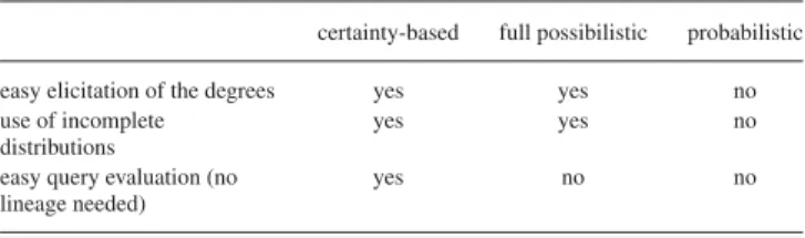
NCERTAIN information may appear in various contexts, such as data warehouses that collect information coming from different sources, automated recognition of objects, sensor networks, forecasts, or archives where only partial information is known for sure. In the database community, the last ten years have witnessed a growing interest in uncertain databases (see, e.g., [1]–[4]). The early works on the topic, however, date back to the late 1970s and early 1980s [5]–[7].Even though most of the literature about uncertain databases uses probability theory as the underlying uncertainty model, this type of modeling is not always so easy, as recognized in the intro-ductory chapter of a key reference book in the field [8]: “Where do the probabilities in a probabilistic database come from? What exactly do they mean? The answer to these questions may dif-fer from application to application, but it is rarely satisfactory.” This is one of the reasons why some authors have proposed ap-proaches that rest on an alternative uncertainty model, namely the possibility theory [9]. The initial idea in applying possi-bility theory to this issue goes back to the early 1980s [10]. More recent advances on this topic can be found in [11]. In contrast with the probability theory, one expects the following advantages when using the possibility theory.
1) The qualitative nature of the model makes the elicitation of the degrees attached to candidate values easier. 2) In the probability theory, the fact that the sum of the
degrees from a distribution must equal 1 makes it difficult to deal with incompletely known distributions.
In this paper, we develop a new idea which is to use the notion of necessity to qualify the certainty that an ill-known piece of
O. Pivert is with IRISA–ENSSAT, University of Rennes 1, Lannion, France (e-mail: [email protected]).
H. Prade is with the Institut de Recherche en Informatique de Toulouse, CNRS, University of Toulouse, 31062 Toulouse, France, and also with the Centre for Quantum Computation and Intelligent Systems, University of Tech-nology, Sydney, N.S.W. 2007, Australia (e-mail: [email protected]).
Digital Object Identifier 10.1109/TFUZZ.2014.2347994
data takes a given value. In contrast with both probabilistic databases and possibilistic ones in the sense of [10] and [11]— which will be referred to as the full possibilistic approach in the following—the main advantage of the certainty-based model lies in the fact that operations from relational algebra can be extended in a simple way and with a data complexity, which is the same as in a classical database context (i.e., where all data are certain).
One of our main aims here is to show how the certainty-based model can be used for expressing a qualitative form of epis-temic uncertainty, which departs from the quantitative additive approach of the probability theory. Let us take the example of a person who witnesses a car accident and is not sure about the model of the car involved. Assume that the person is almost certain that it is a Mazda or a Toyota. Such an uncertain piece of information can be represented by means of a possibility distribution, e.g., {1/Mazda, 1/Toyota, 0.5/others}, where 0.5 is a numerical encoding of an ordinal level in a usually finite possibility scale. Note that it is not a fully specified possibil-ity distribution, since “others” covers unspecified trademarks whose possibility level is upper bounded by 0.5. Note also that in such a case, assessing a probability distribution is more tricky due to the additive normalization condition. As we will see, the previous uncertain piece of information will be simply repre-sented as (Mazda∨ Toyota, 0.5) in the certainty-based model we propose, meaning that we are 0.5 certain that the car observed is either a Mazda or a Toyota.
The remainder of this paper is organized as follows. Section II is devoted to a reminder about basic notions concerning the interpretation of an uncertain database, as well as the prop-erty characterizing a representation system. In Section III, we present the main features of the certainty-based model, and in Section IV, we describe a method that can be used to prove that it is a representation system for a given set of operators. Section V gives the definition of the compact operators (i.e., operators working directly on tables of the model) of relational algebra in this framework. In Section VI, a possibilistic logic encoding of the model is briefly discussed. Section VII presents some related work and includes a comparative discussion with respect to lineage-based methods. An example illustrating the semantics of query results in the three uncertain database mod-els mentioned in this paper, namely the certainty-based one, the full possibilistic one, and the probabilistic one, is given in Section VIII. Section IX recalls the contributions and outlines perspectives for future work.
II. UNCERTAINDATABASE ANDREPRESENTATION
SYSTEMPROPERTY A. Interpretation of an Uncertain Database
The possible worlds model is founded on the fact that un-certainty in data makes it impossible to define what precisely
TABLE I
EXTENSION OFemp (TOP)ANDTWOWORLDSASSOCIATED WITH IT(MIDDLE ANDBOTTOM)
#e name city job
e1 Paul {Chicago, Peoria, Joliet} clerk
e2 David Peoria {clerk, manager}
#e name city job
e1 Paul Chicago clerk
e2 David Peoria clerk
#e name city job
e1 Paul Peoria clerk
e2 David Peoria manager
the real world is. One can only describe the set of possible worlds, which are consistent with the available information. As far as a tableT conveys some imprecision/uncertainty, several interpretations (I) can be drawn from T and the set of all the interpretations ofT is denoted by rep(T ). The notation rep(D) extends naturally to an uncertain databaseD involving several tables. Note that a regular database is a special case of an un-certain one, which has only one interpretation.
Semantically, such an uncertain databaseD can be interpreted in terms of a set of usual databases, which are also called worlds W1, . . . ,Wp, and rep(D) = {W1, . . . ,Wp}. In the following,
we consider the case whererep(D) is finite. Any world Wi is
obtained by choosing a candidate value in each set appearing in a relationTj pertaining toD. One of these (regular) databases,
sayWk, is supposed to correspond to the true state of facts. The
assumption of independence between the sets of candidates is usually made, and then, any worldWi corresponds to a
con-junction of independent choices.
Example 1: Let us consider the uncertain databaseD involv-ing a sinvolv-ingle relationemp whose schema is E(#e, name, city,
job). Relationemp is assumed to describe employees. Let us assume that the city where an employee lives, as well as his/her job, may be ill-known. With the extension ofemp depicted in Table I (top), six worlds can be drawn, that is,W1,W2,W3,
W4,W5, andW6, since there are three candidates for city in the
first tuple and two candidates for job in the second one. Two of the worlds associated with the uncertain relation emp are represented in Table I (middle and bottom).
As we will see in Section III, the or-set model (where re-lations may involve attribute values represented by disjunction of candidates as illustrated in Example 1) may be refined by attaching a weight to every candidate value. The weights may have different semantics, depending on the uncertainty model used.
B. Strong Representation Systems and Compact Calculus
When dealing with an uncertain databaseD, a very important issue is that of the efficiency of the querying process. A naive way of doing would be to make explicit all the interpretations of D (at least when they are finite) in order to query each of them. Such an approach is intractable in practice, and it is of prime
importance to find a more realistic alternative. To this end, the notion of a representation system has been introduced—initially by Imielinski and Lipski [7]—and discussed in [12]. The basic idea is to look for a way for representing both initial tables and those resulting from queries so that the representation of the result of a queryq against any database D (made of tables T1, . . . ,Tp) denoted byq(D) is equivalent (in terms of
interpre-tations, or worlds) to the set of results obtained by applyingq to every interpretation ofD, i.e.,
rep(q(D)) = q(rep(D)) (P1)
where q(rep(D)) = {q(W ) | W ∈ rep(D)}. If property P1 holds for a representation system ρ and a subset σ of the re-lational algebra,ρ is called a strong representation system for σ. From a querying point of view, P1 enables a direct (or compact) calculus of a queryQ, which then applies to D itself without making the worlds explicit. By doing so, provided that relational operations are defined over tables of the system considered, rea-sonable performances can be expected.
III. REPRESENTATION OFUNCERTAINDATA
The aim of this section is to introduce the reader with the certainty-based representation, which is at the basis of the ap-proach proposed in this paper, and to explain its appropriate-ness for expressing epistemic uncertainty. We also point out in what respect the possibilistic representation, of which the certainty-based representation is a particular case, differs from the probabilistic representation.
A. Possibility Theory and Certainty-Based Qualification
In the possibility theory [9], [13], each eventE—which is defined as a subset of a universe Ω—is associated with two measures: its possibilityΠ(E) and its necessity N (E). Π and N are two dual measures, in the sense that N (E) = 1 − Π(E) (where the overbar denotes complementation). This clearly departs from the probabilistic situation, where P rob(E) = 1 − P rob(E). Therefore, in the probabilistic case, as soon as we are not certain about E (P rob(E) is small), we become rather certain aboutE (P rob(E) is large). This is not at all the situation in the possibility theory, where complete ignorance about E (E 6= ∅, E 6= Ω) is allowed: This is represented by Π(E) = Π(E) = 1, and thus, N (E) = N (E) = 0. In the pos-sibility theory, being somewhat certain aboutE (N (E) has a high value) forces you to haveE rather impossible (1 − Π is im-possibility), but it is allowed to have no certainty either aboutE or aboutE. Generally speaking, the possibility theory is oriented toward the representation of epistemic states of information, while probabilities are deeply linked to the ideas of random-ness, and of betting in case of subjective probability, which both lead to an additive model such thatP rob(E) = 1 − P rob(E).
A possibility measure Π (as well as its dual neces-sity measure N ) is based on a possibility distribution π, which is a mapping from a referential U to an or-dered scale, say [0, 1]. Namely, Π(E) = supu ∈E π(u) and
TABLE II
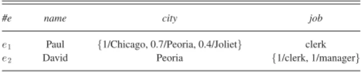
EXTENSION OF THEPOSSIBILISTICRELATIONemp
#e name city job
e1 Paul {1/Chicago, 0.7/Peoria, 0.4/Joliet} clerk
e2 David Peoria {1/clerk, 1/manager}
impossible, whileπ(u) = 1 just means that u is (fully) possi-ble, since it is important to notice that nothing preventsu 6= u′
andπ(u) = π(u′) = 1. Thus, E = {u} is (fully) certain only if
π(u) = 1 and ∀u′6= u, π(u′) = 0. A possibility distribution π
is normalized as soon as∃u, π(u) = 1; it expresses a form of consistency, since it is natural to have at least one alternative fully possible as soon as the referential is exhaustive (this is the counterpart in the possibility theory of having the sum of the probabilities in a probability distribution equal to 1).
Conversely, if we know thatN (E) ≥ α, which means that we are certain (at least) at levelα that E is true, there are several pos-sibility distributions that can be compatible with this constraint, but it can be shown that the largest one (the one that allocates the greatest possible possibility to eachu ∈ U ) is unique and is such thatπ(u) = 1 if u ∈ E and π(u) = 1 − α if u 6∈ E. There-fore, if we areα-certain that Bob lives in Paris or Lyon, this is represented by the distribution π(P aris) = 1 = π(Lyon), andπ(u) = 1 − α for any other city u. If one wants to rep-resent a possibility distribution with more than two levels in terms of constraints of the formN (E) ≥ α, it requires sev-eral constraints. For instance, if it is possible that Peter lives in Brest, Paris, Lyon, or another city with respective possibility levels 1 > α > α′> α′′ (i.e., π(Brest) = 1, π(P aris) = α, π(Lyon) = α′,π(u) = α′′ for any other city u), then it cor-responds to the constraintsN ({Brest, P aris, Lyon}) ≥ 1 − α′′,N ({Brest, P aris}) ≥ 1 − α′andN ({Brest}) ≥ 1 − α.
More generally, any possibility distribution with a finite number of levels1 = α1 > · · · > αn > 0 = αn + 1 can be represented
by a collection ofn constraints of the form N (Ei) > 1 − αi+ 1
withEi= {u | π(u) ≥ αi}.
We further illustrate the use of possibility distributions for representing candidate values for some attributes. Let us con-sider a possibilistic version of the uncertain database from Example 1. In the first tuple ofemp depicted in Table II, Chicago is completely possible and is more possible than Peoria, which is itself more possible than Joliet. Table II corresponds to a rela-tion from the model proposed in [10], while the model proposed in [11] involves an additional attribute expressing the certainty for a tuple to have a representative in any possible world (this makes it possible to represent maybe tuples and is mandatory in order to guarantee property P1).
B. Certainty-Based Representation Used in the Approach
As described in [11], the model we propose is based on the possibility theory [9], but it only represents values that are more
or less certaininstead of those which are more or less possible. This corresponds to the most important part of the information (a possibility distribution is “summarized” by keeping its most
plausible elements). This choice obviously implies a certain loss of information as only the candidate values or disjunctions of candidate values that are somewhat certain are kept. Keep in mind that a statement is all the more certain as its negation is less possible. However, as we shall see, this loss is compensated by a very important gain in terms of query evaluation cost and simplicity/intelligibility of the model. Moreover, the informa-tion lost is quite weak; indeed, when a statement is just possible, its negation is possible as well (otherwise, the statement would be somewhat certain). The idea is to attach a certainty level to each piece of data (by default, a piece of data has certainty 1). Certainty is modeled as a lower bound of a necessity measure. We assume that there always exists a key nonpervaded with uncertainty in base relations. For instance,h037, John, (40, α), (Engineer, β)i denotes the existence of a person named John for sure, whose age is 40 with certainty α, and whose job is
Engineer with certainty β. Then the possibility that his age differs from 40 is upper bounded by1 − α without further in-formation on the respective possibility degrees of other possible values.
In the proposed model, to each uncertain value a of an at-tributeA is attached a certainty degree α. Since the possibility theory is a qualitative framework, one may use an ordinal scale L made of k + 1 linguistic labels to denote the certainty (and possibility) levels attached to an attribute value or a tuple. For instance, withk = 4, one may use
τ0 = “not at all ” < τ1 = “somewhat” <
τ2 = “rather ” < τ3 = “almost” < τ4 = “totally”
whereτ0 (respectively, τk) corresponds to 0 (respectively, 1)
in the unit interval when a numeric framework is used. The operation 1 − (·) that is used when the degrees belong to the unit interval is replaced by the order reversal operation denoted byrev(·): rev(τi) = τk −i.
In the following, in order to have notations that are not too heavy, which could confuse the reader, we will use the fol-lowing numeric scale:τ0 = 0 < τ1 = 0.1 < τ2 = 0.2 < · · · <
τ9= 0.9 < τ10 = 1, and then, rev(τi) = 1 − τi.
The underlying possibility distribution associated with an uncertain value (a, α)—where α ∈ L\{τ0}, \ denoting
set-oriented difference—is {1/a, rev(α)/ω}, where ω denotes domain(A)\{a} (due to the duality necessity/possibility: N (a) ≥ α ⇔ Π(ω) ≤ rev(α) [13]). For instance, let us assume that the domain of the attribute city is domain(city)= {Newton,
Quincy, Boston}. The uncertain attribute value (Newton, α) is assumed to correspond to the possibility distribution{1/Newton, rev(α)/Quincy, rev(α)/Boston}. More generally, the model can deal with disjunctive values, and the underlying possibility dis-tributions are of the form
{max(µS(x1), rev(α))/x1, . . . , max(µS(xp), rev(α))/xp}
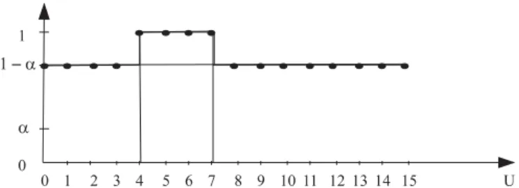
where S is an α-certain subset of the attribute domain, and µS(xi) equals 1 if xi∈ S, 0 otherwise [14]. Fig. 1 shows
the possibility distribution associated with the uncertain value ({4, 5, 6, 7}, α), assuming that the corresponding domain is U = {0, . . . , 15}.
Fig.1. Possibility distribution associated with the uncertain value ({4, 5, 6, 7}, α).
TABLE III
RELATIONSr (TOP)ANDs (BOTTOM)
#id name city N
37 John (Newton,α ) 1
53 Mary (Quincy,δ ) 1
city flea market N
Newton (yes,β ) 1
Quincy (no,γ ) 1
Moreover, since some operations (e.g., the selection) may create “maybe tuples” (i.e., tuples whose existence in the result is itself uncertain), each tuplet from an uncertain relation r has to be associated with a degreeN expressing the certainty that t exists inr. It will be denoted by N/t.
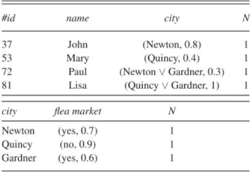
Example 2: Let us consider the relationr of schema (#id,
name, city) —plus the extra attributeN that represents the cer-tainty degree attached to the tuple, as mentioned above—from Table III and the query “find the persons who live in Newton.” Let the domain of attribute city be domain(city) = {Newton,
Quincy, Boston}. The answer contains α/t1 (wheret1 denotes
the first tuple ofr), since it is α-certain that t1 satisfies the
re-quirement, while the result of the query “find the persons who live in Boston, Newton, or Quincy” contains 1/t1, since it is
totally certain thatt1 satisfies the condition (this is also true for
t2, by the way).⋄
To sum up, a tuple of the form λ/h37, John, (Newton, α)i from relationr means that it is λ-certain that person 37 exists in the relation, that it is totally sure that the name of that person is John, and that it isα-certain that person 37 lives in Newton (independently from the fact that it is or not in relationr).
Given a query, we only look for answers that are somewhat
certain:We are not interested in answers that are just possible, which makes the approach much more simple. Notice, however, that potential answers that are omitted are precisely those for which it is certain to some degree that they are in fact not an answer. However, not having them is not a great loss for the user. Consider the relations from Table III and a query asking for the persons who live in a city with a flea market. John will be retrieved with a certainty level equal tomin(α, β) (in agreement with the calculus of necessity measures [14]). Although it is not impossible that Mary lives in a city with a flea market, she does not belong to the answer because her living in such a city is just possible and not certain (even partially).
As mentioned in Section I, it is an acknowledged fact that databases often contain a nonnegligible amount of suspect tu-ples. This is due either to the fact that after some time, an originally true piece of information may become false (because the world has changed), or because the database is fed by mul-tiple sources or experts that may have conflicting views or in whom one may have different confidence levels. Even when this state of fact is known in a database, getting rid of all the suspects tuples would be much too costly in general. Rather, alerting the user by indicating that some information has a smaller certainty level (because, e.g., the information is not recent) seems a better strategy. For instance, taking the example above, the fact that a flea market exists in a city may have become somewhat un-certain because the information has not been refreshed recently, but it is usually easier for the user who is often interested in a rather small number of the answers received to check them, once he has been warned by the lack of full certainty associated with some answers of interest.
As mentioned above, it is also possible to handle cases of disjunctive information in this setting. For instance,h3, Peter, (Gardner∨ Fitchburg, α)i represents the fact that it is α-certain that the person number 3 named Peter lives in Gardner or in
Fitchburg. On the other hand, notice that one cannot have in relationr two tuples like h1, John, (Boston, α)i and h1, John, (Newton, β)i. Indeed, according to the possibility theory, two different individual values cannot be somewhat certain at the same time.
IV. REPRESENTATIONSYSTEMPROPERTY IN THE
CERTAINTY-BASEDCASE
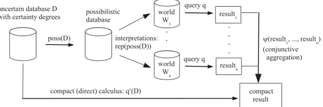
Let us now examine what becomes of property P1 in such a context. Let us denote by D an uncertain database involv-ing certainty levels, andposs(D) the corresponding uncertain database involving possibility distributions, i.e., one of the form of Table II but with the possibility distributions computed from the uncertain inputs as described in Section III-B (just before Example 2). Let us also denote byq an algebraic query, and qc
the compact version ofq. The counterpart of property P1 is
qc(D) = ψ(q(rep(poss(D)))) (P2)
whereψ(r′) denotes the certainty-based relation, which gathers the tuples somewhat certainly in the intersection of all the (more or less) possible worlds from the set r′ (each world from r′
represents a possible result ofq applied to poss(D)). Property P2 is graphically represented in Fig. 2. This property is similar to the weak representation system property [12] defined as
sure(q, D) = ∩{q(I) | I ∈ rep(D)}
which requires that the table resulting from a queryq represents the tuples that are surely in the answer toq. However, in the case of the certainty-based model, the distinction between a strong and a weak representation system no longer really makes sense: The model is by its very nature restricted to the representation of events (values, tuples from initial relations or query answers) that are somewhat certain.
Fig. 2. Compact query evaluation (Property P2).
Operationψ works as follows. First, one attaches an identi-fier to every tuple fromD involving at least one uncertain value (this is necessary whenq involves a projection which removes the keys). Note that this identifier is virtual and does not impact the result of the operations performed on the worlds (intersection and difference, in particular). When duplicates are eliminated in a world, the list of identifiers attached to the tuples merged is attached to the tuple resulting from the merging. Each world W of rep(poss(D)) is associated with a valuation V describ-ing the value taken inW by each attribute of each uncertain tuple from the initial uncertain databaseD. When V(id) = ∅ in a given worldW , this means that the world has been built by choosing no representative of the uncertain tuple identified byid (which implies that the certainty degree attached to this tuple was less than 1 in the initial database). To illustrate this, let us consider the databaseD made of the uncertain relation r = {0.9/h17, John, (Boston, 0.7)i, 0.8/h53, Peter, (Newton, 0.4)i} and the selection query based on the condition city = “Boston.”
In the following, eachΠivalue corresponds to the possibility
of the associated world, which is denoted byWi. It is equal to
the minimum of the possibility degrees attached to the choices that have been made, in terms of tuples, to build the world. The possibility degree attached to a tuple is the minimum of the possibility degrees attached to the values that it involves (the latter being 1 if the value appeared as somewhat certain, 1 minus the degree attached to the value—or disjunction of values—that appeared as somewhat certain otherwise). The possibility that a tuple be absent (i.e., that a tuple fromD have no representative inposs(D)) is 1 minus the certainty degree attached to this tuple in the initial certainty-based representation. The worlds of rep(poss(D)) are
W1 = {h17, John, Bostoni, h53, Peter, Newtoni}, with Π1
= 1, V(17) = hBostoni, V(53) = hNewtoni.
W2 = {h17, John, ǫ1i, h53, Peter, Newtoni}, with Π2
= min (1 - 0.7, 1) = 0.3,V(17) = hǫ1i, V(53) = hNewtoni.
W3 = {h17, John, Bostoni, h53, Peter, ǫ2i}, with Π3
= min (1, 1 - 0.4) = 0.6, V(17) = hBostoni, V(53) = hǫ2i.
W4 = {h17, John, Bostoni}, with Π4 = min(1, 1 − 0.8)
= 0.2, V(17) = hBostoni, V(53) = ∅.
W5 = {h17, John, ǫ1i}, with Π5 = min(1 − 0.7, 1 − 0.8)
= 0.2, V(17) = hǫ1i, V(53) = ∅.
W6 = {h53, Peter, Newtoni}, with Π6 = min(1 − 0.9, 1)
= 0.1, V(17) = ∅, V(53) = hNewtoni.
W7 = {h53, Peter, ǫ2i}, with Π7 = min(1 − 0.9, 1 − 0.4)
= 0.1, V(17) = ∅, V(53) = hǫ2i.
W8 = {h17, John, ǫ1i, h53, Peter, ǫ2i}, with Π8 = min
(1 – 0.7, 1– 0.4)= 0.3, V(17) = hǫ1i, V(53) = hǫ2i.
W9 = ∅, with Π9 = min(1 − 0.9, 1 − 0.8) = 0.1, V
(17)= ∅, V(53) = ∅.
Here,ǫ1 (respectively, ǫ2) ∈ domain(city)\{Boston}
(re-spectively,domain(city)\{N ewton}). For each tuple present in a world fromq(rep(poss(D))), denoting by id its identifier— or (id1,id2) in case of a binary operation—one has to check the
following:
1) whether there exists a completely possible world from q(rep(poss(D))) from which id—or (id1,id2) for a join,
id1 and/orid2 for an intersection,id1 for a difference—
is absent. If it is the case,ψ(q(rep(poss(D)))) does not contain any tuple identified byid;
2) otherwise
a) the certainty degree associated with the “compact tuple” produced is equal to 1 minus the maximal possibility degree associated with a world from whichid is absent;
b) for each attributeA of the result, one gathers into a disjunctionVA(id) the values associated with id in
the completely possible worlds of the result; the cer-tainty degree associated withVA(id) equals rev(τ ),
whereτ is the maximal possibility degree attached to a world ofq(rep(poss(D))) such that either 1) id is present andV(id).A /∈ VA(id) or 2) id is absent
andV(id) 6= ∅.
In the previous example, the worlds of the result are the following:
W1′= {h17, John, Bostoni}, with Π1 = 1, V(17) = hBostoni,
V(53) = hNewtoni. W′
2 = ∅, with Π2 = 0.3, V(17) = hǫ1i, V(53) = hNewtoni.
W′
3 = {h17, John, Bostoni, h53, Peter, Bostoni}, with
Π3 = 0.6, V(17) = V(53) = hBostoni.
W′
4 = {h17, John, Bostoni}, with Π4 = 0.2, V(17) =
hBostoni, V(53) = ∅. W′ 5 = ∅, with Π5 = 0.2, V(17) = hǫ1i, V(53) = ∅. W′ 6 = ∅, with Π6 = 0.1, V(17) = ∅, V(53) = hNewtoni. W′
7 = {h53, Peter, Bostoni}, with Π7= 0.1, V(17) = ∅,
V(53) = hǫ2i.
W′
8 = {h53, Peter, Bostoni}, with Π8 = 0.3, V(17) = hǫ1i,
W′
9= ∅, with Π9 = 0.1, V(17) = ∅, V(53) = ∅.
The certainty degree associated with tuple 17 in the compact result equals
1 − max(Π2, Π5, Π6, Π7, Π8, Π9) = 1 − 0.3 = 0.7.
As to tuple 53, it is not in the result since there is a com-pletely possible world (W′
1) in which 53 is absent. The
certainty degree associated with Boston in tuple 17 equals 1 − max(Π2, Π5, Π8) = 1 − 0.3 = 0.7. Indeed, according to
the definition above, it equalsrev(τ ), where τ is the maximal possibility degree attached to a world ofq(rep(poss(D))) such that either tuple 17 is present and V(17).city /∈ Vcity(17) =
{Boston} (but there is no such world) or tuple 17 is absent andV(id) 6= ∅ (case of the worlds W′
2,W5′,W8′). Finally, the
compact result is{0.7/h17, John, (Boston, 0.7)i}. V. RELATIONALALGEBRAOPERATORS
The goal of this section is to define the compact version of the relational algebraic operators and to show that the certainty-based database model is a representation system for this set of operators, i.e., that property P2 holds. The only limitation w.r.t. the usual algebraic framework consists of the fact that the operands of the Cartesian product and the join must be indepen-dent relations (we mean here that they must not stem from the same initial relation, which forbids self-joins). Otherwise, one would have to represent intertuple constraints, which is beyond the capabilities of the model in its current form. This point will be illustrated further in the section devoted to the join operation.
A. Selection
Let us consider a relationr of schema (A, X), where A is an attribute andX is a set of attributes, and a selection condition φ on A. Let us denote by s(t.A) the disjunctive set of values— which may be a singleton—somewhat certain for attributeA in tupleµ/t, and by c(t.A) the associated certainty level. Let us first deal with the case whereφ writes A θ q, where θ denotes a comparator andq a constant
σA θ qc (r) =
½
µ′/t | ∃µ/t ∈ r such that ∀ai∈ s(t.A), aiθ q
and µ′=
min(µ, 1) = µ if ∀ai ∈ domain(A), aiθ q;
min(µ, c(t.A)) otherwise ¾
.
Let us prove that property P2 holds with this definition of the selection, i.e., that
σc
A θ q(r) = ψ(σA θ q(rep(poss(r)))).
Proof: As the selection operates on tuples individually, one can assume that r contains only one tuple. Let us de-note it byµ/t and assume that s(t.A) = (a1∨ a2∨ · · · ∨ an)
and c(t.A) = α. Let us attach an identifier id to this tu-ple. Let us recall that the maximal possibility distribution
as-sociated with s(t.A) is {1/a1, 1/a2, . . . , 1/an, 1 − α/ω},
where ω = domain(A) − {a1, , a2, . . . , an}. Three cases
may appear.
1) ∃ai∈ {a1, a2, . . . , an} such that ¬(aiθ q): then, there
exists a completely possible world of the result where id is not present. The certainty degree attached to id is 0, andψ(σA θ q(rep(poss(r)))) is empty, which is consistent
with the definition above.
2) ∀ai∈ domain(A), aiθ q: then, id is present in every
completely possible world and the only possible world where id is not present is the empty world (possi-bility rev(µ)). Hence, the certainty degree attached to id in ψ(σA θ q(rep(poss(r)))) is rev(rev(µ)) = µ. The
most possible world where id has an A-value which does not belong to s(t.A) in the result has the pos-sibility degree rev(α). Hence, the certainty degree at-tached to theA-value s(t.A) in the tuple identified by id inψ(σA θ q(rep(poss(r)))) is rev(rev(α)) = α. This is
consistent with the compact definition of selection where s(t.A) and c(t.A) are kept unchanged.
3) ∀ai∈ {a1, a2, . . . , an}, aiθ q and ∃ui∈ domain(A) such that¬(uiθ q): then, id is present in every completely
possible world. The most possible world whereid is not present is either the empty world (possibilityrev(µ)) or is made of a tuplehid, ui,t.Xi where ui∈ ω (possibility
rev(α)). Thus, this most possible world has the possibil-ity degree max(rev(µ), rev(α)). Hence, the certainty degree attached to id in ψ(σA θ q(rep(poss(r)))) is
rev(max(rev(µ), rev(α))) = min(µ, α). The most possible world where id has an A-value which does not belong to s(t.A) in the result has the possibility degree rev(α). Hence, the certainty degree attached to the A-value s(t.A) in the tuple identified by id in ψ(σA θ q(rep(poss(r)))) is rev(rev(α)) = α. This is
consistent with the compact definition above. ¥
Let us now consider a conditionφ of the form A1θ A2, where
A1andA2denote two attributes. The definition of the selection
in this case is σcA1θ A2(r) =
½
µ′/t | ∃µ/t ∈ r such that
∀a1,i ∈ s(t.A1), ∀a2,j ∈ s(t.A2), a1,iθ a2,jand
µ′=
µ if ∀(u, v) ∈ dom(A1) × dom(A2), u θ v;
min(µ, c(t.A1), c(t.A2)) otherwise
¾ .
The proof is omitted since it is very similar to that given for the previous case.
From the previous definitions, it immediately follows that the data complexity of the selection operation is linear (as usual). The example hereafter illustrates the case of a conjunctive se-lection condition.
Example 3: Let us consider the database D made of the sole
relation emp of schema (id, name, city, job). Let us suppose that emp only contains tuple t = 0.9/h17, John, (Boston, 0.8), (Engineer, 0.7)i, and let us consider the query: q = σcity=
‘Boston’ and job = ‘Engineer’ (emp). Its compact result is 0.7/h17, John, (Boston, 0.8), (Engineer, 0.7)i. Let us show that property P2 is satisfied. Identifier 17 is present in ev-ery completely possible world of the result. The most possi-ble world of emp where 17 is not present in the result of the selection is made of the tuple h17, John, Boston, ǫ)i (where ǫ ∈ ω = domain(job)\{Engineer}) and has the possibility degree min(1, 1 − 0.7) = 0.3. Hence, the certainty degree at-tached to 17 in the result is 1 − 0.3 = 0.7. The most possible world where 17 has a city value different from Boston in the result has the possibility degree 1 − 0.8 = 0.2. Hence, the cer-tainty degree attached to the city value Boston in the tuple identified by 17 in the result is 1 − 0.2 = 0.8. The most possi-ble world where 17 has a job value different from Engineer in the result has the possibility degree 1 − 0.7 = 0.3. Hence, the certainty degree attached to the job value Engineer in the tu-ple identified by 17 in the result is 1 − 0.3 = 0.7. The compact calculus is thus correct.⋄
B. Join
1) Definition: The compact definition of the join in the con-text of the certainty-based model is
r1⊲⊳cA =B r2 = {min(α, β, χ, δ)/t1⊕ t2
∃α/t1 ∈ r1, ∃β/t2 ∈ r2 such that
card(s(t1.A)) = 1 and card(s(t2.B)) = 1 and (1)
s(t1.A) = s(t2.A) and c(t1.A) = χ and c(t2.B) = δ}
where⊕ denotes the concatenation, and card returns the cardi-nality of a set. Notice that only the tuples whose value for the join attribute is nondisjunctive (i.e., is a singleton) can partici-pate in the result: For the other ones, one cannot be certain at all that they match a tuple from the other relation. Indeed, for a tuplet1 ofr whose join attribute value t1.A is disjunctive, it
is always possible to find a completely possible interpretation such that the (equi-)join condition is false, whatever the tuple t2 froms. The proof is omitted as it is rather cumbersome, but
the example hereafter illustrates the way it works. Note that this property would not hold in the case of aθ-join, where θ is not equality.
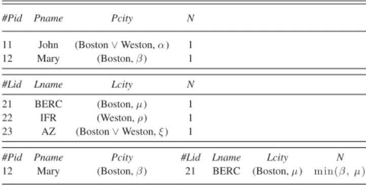
Example 4: Consider the relations Person and Lab from Ta-ble IV and the query:
P ersLab = P erson ⊲⊳cP city =L city Lab
which looks for the pairs (p, l) such that person p (somewhat cer-tainly) lives in a city in which a research centerl is located. Let us show that the result of the compact join is correct using the same method as we did in Section IV for the selection. The only pair of identifiers present in every completely possible world is (12, 21). The most possible world where (12, 21) is not present has the possibility degree min(max(rev(β), rev(µ)), 1) = max(rev(β), rev(µ)) = rev(min(β, µ)). Hence, the certainty degree attached to (12, 21) in the result ismin(β, µ). The most
TABLE IV
RELATIONSP erson (TOP),Lab (MIDDLE),ANDP ersLab (BOTTOM)
#Pid Pname Pcity N
11 John (Boston∨ Weston, α) 1 12 Mary (Boston,β ) 1
#Lid Lname Lcity N
21 BERC (Boston,µ) 1 22 IFR (Weston,ρ) 1 23 AZ (Boston∨ Weston, ξ ) 1
#Pid Pname Pcity #Lid Lname Lcity N
12 Mary (Boston,β ) 21 BERC (Boston,µ) m in(β , µ)
possible world where (12, 21) has a Pcity value different from
Boston has the possibility degree min(rev(β), 1) = rev(β). Hence, the certainty degree attached to theP city value Boston in the tuple identified by (12, 21) in the result isβ. The most possi-ble world where (12, 21) has an Lcity value different from Boston has the possibility degreemin(rev(µ), 1) = rev(µ). Hence, the certainty degree attached to theLid value Boston in the tuple identified by (12, 21) in the result isµ. Notice that in the case of an equi-join—as it is the case here—both columnsP id and Lid could be merged into a single column in the resulting table.
Johncannot take part to the result since one cannot be certain of what theLab value associated with him is.⋄
2) About the Semi-Join Operation: An interesting remark about the preceding example is that, even though the result of the join does not contain any tuple involving John, this individual belongs to the result of the semi-join which looks for the persons who (somewhat certainly) live in a city where a research center is located: Person ⋉ Lab. This means that the usual equivalence between a semi-join and a join followed by a projection, i.e., r1⋉ r2≡ πX(r1⊲⊳r2), where X denotes the attributes of r1,
is not valid anymore in the context of the certainty-based model. However, the semi-join can be defined in a sound way in this framework. Informally, for a tuplet1fromr1to be in the result
of the semi-joinr1⋉ r2, each valueai froms(t1.A) has to be
present as a singletonB-value in a tuple from r2. If anaifrom
s(t1.A) joins with several tuples from r2, the maximum of the
corresponding certainty degrees must be used for computing the certainty degree attached to t1 in the result. The formal
definition is
r1⋉cA θ Br2 = {min(µ, α, min i= 1..n
λi)/t1) | ∃µ/t1∈ r1such thats(t1.A) = {a1, . . . , an} and
c(t1.A) = α and
∀ai∈ s(t1.A), (∃t2j ∈ r2 s.t. s(t2j.B) = {ai}) and (2)
λi= max
j | δj/t2 j∈r2∧s(t2 j.B )={ai}∧c(t2 j.B )=βj
min(δj, βj)}.
Using this definition and the relations from Table IV, the re-sult of the semi-join expressed above is given in Table IX. Note that the tuple#Lid = 23 in Table IV has no influence on the result, since taking into account tuple#P id = 11, John
TABLE V
DEPENDENCE IN THERESULT OF ASELF-JOINQUERY
#Pid1 Pname1 Pcity1 Pname2 Pcity2 N
11 John (Boston∨ Weston, α) John (Boston∨ Weston, α) 1 12 Mary (Boston,β ) Mary (Boston,β ) 1
may live in Boston, while the AZ lab may be in Weston (or the converse).
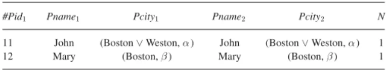
3) About the Self-Join Operation: As mentioned in the be-ginning of this section, self-joins cannot be handled in this model, since the presence of several copies of the same relation may induce dependences between uncertain attribute values. Let us consider, for instance, the relation Person from Table IV and the self-join queryQ = Person1 ⊲⊳# P id= # P id Person2.
Its result, represented in Table V—let us denote it byres— shows that a dependence exists in the first tuple between the value ofP City1and that ofP City2. Indeed, when the worlds
associated withposs(res) are built, the same candidate value must be chosen forP City1 andP City2 in this tuple, but this
dependence is not captured by the model.
C. Projection
Letr be a relation of schema (X, Y ). The projection operation is straightforwardly defined as follows:
πXc (r) = {α/t.X | α/t ∈ r and
6 ∃α′/t′∈ r such that sbs(α′/t′.X, α/t.X)}. The only difference w.r.t. the definition of the projection in a classical database context concerns duplicate elimination, which is here based on the concept of “possibilistic subsumption.” LetX = {A1, . . . , An}. The predicate sbs, which expresses
subsumption, is defined as follows: sbs(α′/t′.X, α/t.X) ≡
∀i ∈ {1, . . . , n}, s(t.Ai) = s(t′.Ai) and
c(t.Ai) ≤ c(t′.Ai) and α ≤ α′and
((∃i ∈ {1, . . . , n}, c(t.Ai) < c(t′.Ai)) or α < α′).
The validity of the result before duplicate removal is guaranteed by the satisfaction of P2. As to the duplicate removal step, its soundness relies on the axioms of possibility theory.
D. Cartesian Product
Letr1 (respectively,r2) be a relation of schema(X, A)
(re-spectively,(Y, B)) with A and B two compatible sets of at-tributes. The Cartesian product is defined as follows:
r1×cr2 = {min(α, β)/t1⊕ t2|
∃α/t1 ∈ r1 and ∃β/t2∈ r2}
where⊕ denotes the concatenation. It is straightforward to prove that the definition of the join and that of the Cartesian product guarantee the equivalence (similar to that which exists in the
TABLE VI
RELATIONSr1(TOP),r2(MIDDLE),ANDr1∪cr2(BOTTOM)
Job City N
(Engineer, 0.6) (Boston, 0.7) 1 (Engineer∨ Manager, 0.7) (Boston, 0.8) 0.7 Manager Newton 1
Job City N
(Engineer∨ Manager, 0.9) Boston 0.9 Manager Newton 1 (Engineer, 0.8) (Boston, 0.4) 0.4
Job City N
(Engineer, 0.6) (Boston, 0.7) 1 Manager Newton 1 (Engineer∨ Manager, 0.9) Boston 0.9 (Engineer, 0.8) (Boston, 0.4) 0.4
classical case):
r1 ⊲⊳A =B r2 ≡ πA(σA =B(r1× r2)). E. Union
Union is defined as usual (and has the same data complex-ity), except that duplicate elimination is based on the notion of “possibilistic subsumption” (see Section V-C).
Example 5: Consider the relations from Table VI . The sec-ond tuple of relationr1is subsumed by the first tuple of relation
r2, which is the only one kept. ⋄
F. Intersection
The intersectionr1∩cr2 is defined as follows: A tuplet of
r1 (respectively,r2)—in the sense of its attribute values—is in
the result iff all of its interpretations are inr2(respectively,r1).
The formal definition is
r1∩cr2 = inter(r1, r2) ∪ inter(r2, r1)
where
inter(r, r′) = {min(µ1, min
k µk)/h(t.A1, min(ρ1,1, mink ρk ,1)), . . .
(t.An, min(ρ1,n, min
k ρk ,n))i |
µ1/h(t.A1, ρ1,1), . . . , (t.An, ρ1,n)i ∈ r and
∀tk ∈ rep(t), ∃µk/h(tk.A1, ρk ,1), .., (tk.An, ρk ,n)i ∈ r′}. Proof: Let us show that property P2 holds. For the sake of clarity, we will assume that relations r1 and r2 involve
only one attribute A (the extension to the multiple attribute case is straightforward). Let us assume that r1 contains a
tu-plet1 = µ1/(a1,1∨ · · · ∨ a1,n, α1). For (a1,1∨ · · · ∨ a1,n) to
be in the compact result of the intersectionr1∩ r2, it is
neces-sary that the disjunction (a1,1∨ · · · ∨ a1,n) be somewhat
cer-tainly in r1∩ r2. This implies that in each completely
possi-ble world of the result, there exists eithera1,1 or. . . or a1,n.
TABLE VII
RELATIONSr1(TOP),r2 (MIDDLE),ANDr1∩cr2 (BOTTOM)
Job City N
(Engineer, 0.6) (Boston, 0.7) 1 (Engineer∨ Clerk, 0.7) (Boston∨ Newton, 0.8) 0.7 (Technician, 0.7) Boston 0.8 Technician (Quincy, 0.3) 1 Job City N (Engineer, 0.9) (Boston, 0.4) 0.9 (Engineer, 0.6) (Newton, 0.3) 1 (Clerk, 0.5) Boston 0.7 (Clerk, 0.2) (Newton, 0.6) 0.4 Technician (Boston∨ Quincy, 0.4) 0.5
Job City N
(Engineer, 0.6) (Boston, 0.4) 0.9 (Engineer∨ Clerk, 0.2) (Boston∨ Newton, 0.3) 0.4 (Technician, 0.7) (Boston∨ Quincy, 0.3) 0.5
µ2,i/(a1,i, α2,i) in r2. Then, the necessity degree attached to
the tuple (a1,1∨ · · · ∨ a1,n, α) in the compact result equals
min(µ1, minj = 1,...,n µ2,j). Indeed, the most possible world
where the intersection contains no representative oft1 has the
possibility degree max(rev(µ1), max j = 1,...,nrev(µ2,j)) = rev(min(µ1, min j = 1,...,nµ2,j)). ¥
As to degreeα, it is equal to rev(τ ), where τ is the possibility that the value oft1.A is not in {a11, . . . , a1,n}, i.e.,
rev(max( rev (α1), max
j = 1,...,n rev(α2,j)))
= rev(rev(min(α1, min
j = 1,...,n α2,j)))
= min(α1, min
j = 1,...,n α2,j).
These calculi are consistent with the definition of the intersection above.
As mentioned in Section IV, in the general case where relation r1contains several tuples, one must attach a virtual identifier to
every tuple fromr1 in order to recognize that the differenta1,i
in the completely possible worlds of the result come from the same compact tuple fromr1.
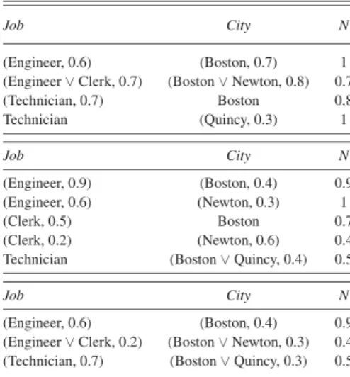
The reciprocal case—which consists in checking whether a tuple fromr2is in the intersection—is symmetrical. ¥ Example 6: Consider the relations from Table VII .r1∩cr2
contains a tuple of the formµ/h(Engineer, α), (Boston, β)i, since such a tuple exists in both relations. On the other hand, tupleµ/hTechnician, (Quincy, 0.3)i from r1is not in the result,
since there is no corresponding tuple inr2 (but its existence
along with that of 0.8/h(Technician, 0.7), Bostoni explains why the last tuple ofr2is in the result.⋄
TABLE VIII
RELATIONSr1(TOP),r2 (MIDDLE),ANDr1−cr2(BOTTOM)
Job City N
(Engineer∨ Clerk, 0.7) (Boston∨ Newton, 0.8) 0.6 (Engineer, 0.6) (Quincy∨ Boston, 1) 0.7
Job City N
(Engineer, 0.5) (Newton, 0.9) 0.4 (Clerk, 0.2) (Quincy∨ Nantes, 0.6) 0.9 (Cashier∨ Clerk, 0.4) Boston 0.2
Job City N
(Engineer, 0.6) (Quincy∨ Boston, 1) 0.2
G. Difference
Let us now consider the differencer1−cr2. Letµ/t be a tuple
fromr1. One must determine the extent to which it is certain that
t is different from every tuple from r2. In other words, one must
compute the degree of certaintyδ that none of the interpretations tkoft is in r2. Let us denote by{µ2,1/t2,1, . . . , µ2,n/t2,n} the
tuples from r2 and by (A1, . . . , Ap) the schema of both r1
andr2: δ = min k N (tk ∈ r/ 2) = min k N (t2,16= tk and. . . and t2,n6= tk) = min k min(N (t2,16= tk), . . . , N (t2,n 6= tk)) = min k min(max(rev(Π(t2,1 = tk)), rev(µ2,1)), . . . max(rev(Π(t2,n = tk)), rev(µ2,n))).
The termrev(µ2,j) is there to take into account the possibility
thatt2,jmay not exist inr2. One has
Π(t2,i = tk)
= Π(t2,i.A1= tk.A1 and . . . and Π(t2,i.Ap = tk.Ap)
= min(Π(t2,i.A1 = tk.A1), . . . , Π(t2,i.Ap = tk.Ap))
Π(t2,i.Aj = tk.Aj)
= 1 if tk.Aj ∈ s(t2,i.Aj), rev(c(t2,i.Aj)) otherwise.
Finally, ifδ 6= 0, t belongs to r1−cr2with the certainty degree
min(µ, δ).
Example 7: Consider the relationsr1andr2from Table VIII.
The first tuple ofr1, which is denoted by t1,1, has four
inter-pretations, among whichhEngineer, Newtoni which is present inr2. Thus,δ equals 0 and this tuple is discarded. The second
tuple of r1, which is denoted byt1,2, has two interpretations:
t′
1 = hEngineer, Quincyi and t′2 = hEngineer, Bostoni. Let us
first compute the degree of certainty thatt′
1 is not inr2. Let us
denote byt2,1,t2,2, andt2,3the first, second, and third tuple of
r2, respectively. We have
Π(t2,1 = t′1) = min(1, 1 − 0.9) = 0.1
N (t2,16= t′1) = max(1 − 0.1, 1 − 0.4) = 0.9
TABLE IX
RESULT OF THECOMPACTSEMI-JOINQUERY
#Pid Pname Pcity N
11 John (Boston∨ Weston, α) m in(α , µ, ρ) 12 Mary (Boston,β ) m in(β , µ)
N (t2,26= t′1) = max(1 − 0.8, 1 − 0.9) = 0.2 Π(t2,3 = t′1) = min(1 − 0.4, 1 − 1)) = 0 N (t2,36= t′1) = max(1 − 0, 1 − 0.2) = 1 min(N (t2,1 6= t′1), N (t2,2 6= t′1), N (t2,36= t′1)) = 0.2. Similarly, we obtain min(N (t2,1 6= t′2), N (t2,2 6= t′2), N (t2,36= t′2)) = 0.6.
Thus,δ = min(0.2, 0.6) = 0.2 and t1,2belongs tor1−cr2
with the certainty degreemin(0.7, 0.2) = 0.2. ⋄
H. About Query Equivalences
Let us recall that relational algebraic queries can be repre-sented as a tree where the internal nodes are operators, leaves are relations, and subtrees are subexpressions. The primary goal of query optimization is to transform expression trees into equiv-alent ones, where the average size of the relations yielded by subexpressions in the tree is smaller than they were before the optimization. This transformation process uses a set of proper-ties (query equivalences), and the question arises as to whether these properties remain valid in the certainty-based model. The most common query equivalences are the following:
1) πX(πX Y(r)) = πX(r). 2) σψ2(σψ1(r)) = σψ1(σψ2(r)) = σψ1∧ ψ2(r). 3) σψ1∨ ψ2(r) = σψ1(r) ∪ σψ2(r). 4) σψ(πX(r)) = πX(σψ(r)) if ψ concerns X only. 5) σψ(r1× r2) = σψ1∧ ψ2∧ ψ3(r1× r2) = σψ3(σψ1(r1) × σψ2(r2)), where ψ = ψ1 ∧ ψ2 ∧ ψ3
andψ1 concerns only attributes from r1,ψ2 concerns
only attributes from r2, and ψ3 is the part of ψ that
concerns attributes from bothr1andr2.
6) σψ(r1∪ r2) = σψ(r1) ∪ σψ(r2). 7) σψ(r1∩ r2) = σψ(r1) ∩ σψ(r2) = σψ(r1) ∩ r2 = r1∩ σψ(r2). 8) σψ(r1− r2) = σψ(r1) − σψ(r2) = σψ(r1) − r2. 9) πX(r1∪ r2) = πX(r1) ∪ πX(r2). 10) πZ(r1× r2) = πX(r1) × πY(r2) if X (respectively, Y )
denotes the subset of attributes of Z present in r1
(respectively,r2).
It is straightforward to prove that all of these equivalences remain valid in the certainty-based model (they are direct con-sequences of the definitions of the operators given above).
VI. POSSIBILISTICLOGICENCODING OF THEMODEL
As already recalled, possibility theory associates two mea-sures to a formulaϕ (describing an event), namely its possibil-ityΠ(ϕ), which estimates how unsurprising the formula ϕ is (Π(ϕ) = 0 means that ϕ is bound to be false) and its dual ne-cessityN (ϕ) = 1 − Π(¬ϕ) (N (ϕ) = 1 means that ϕ is bound
to be true). A standard possibilistic logic [15], [16] expres-sion is a pair(ϕ, α), where ϕ is a classical logic formula and α ∈ (0, 1] is interpreted as a lower bound of a necessity mea-sureN , i.e., (ϕ, α) is semantically interpreted as N (ϕ) ≥ α, whereN is a necessity measure. Necessity obeys the charac-teristic axiomN (ϕ ∧ ψ) = min(N (ϕ), N (ψ)). Thanks to this decomposability property, a possibilistic logic base (i.e., a con-junction of possibilistic formulas) can always be put in a clausal equivalent form (i.e., a collection of weighted clauses), since N (ϕ ∧ ψ) ≥ α is equivalent to N (ϕ) ≥ α and N (ψ) ≥ α.
The fact that we only consider here sets of constraints of the formN (ϕ) ≥ α means that we only represent the upper bound of the family of possibility distributions that are compatible with these constraints. Note that we do not consider here any piece of information of the formN (ϕ) ≤ α ⇔ Π(¬ϕ) ≥ 1 − α. The joint use of the two types of constraints would enable us to represent a possibility distribution exactly, but lead to a more general possibilistic logic whose computational complexity is higher [16]. After a brief reminder on possibilistic logic, we explain how database querying is handled in basic possibilistic logic, whose inference complexity [17] remains close to that of classical logic, due to the application of a local rule of resolution.
A. Reminder About Possibilistic Logic
A possibilistic knowledge base is a setK = {(ϕi, αi), i =
1 . . . n}, where ϕi is a propositional logic formula and its cer-taintylevel (or weight)αiis such thatN (ϕi) ≥ αi,N being a
necessity measure.
The following resolution rule [15] is valid in possibilistic logic:
(a ∨ b, α); (¬a ∨ c, β) ⊢ (b ∨ c, min(α, β))
where⊢ denotes the syntactic inference of possibilistic logic. Classical resolution is retrieved when all weights are equal to 1. The resolution rule allows us to compute the maximal certainty level that can be attached to a formula according to the constraints expressed by the baseK. This can be done by adding to K the clauses obtained by refuting the proposition to evaluate, with a necessity level equal to 1. Then, it can be shown that any lower bound obtained on⊥, by resolution, is a lower bound of the necessity of the proposition to evaluate. LetInc(K) = max{α | Kα ⊢ ⊥} with Kα = {f | (f, β) ∈ K
andβ ≥ α}, with the convention max(∅) = 0. In case of partial inconsistency of K (Inc(K) > 0), a refutation carried out in a situation where Inc(K ∪ {(¬f, 1)}) = α > Inc(K) yields the nontrivial conclusion (f, α), only using formulas whose certainty levels are strictly greater than the level of inconsis-tency of the base.
Using this rule repeatedly, in a refutation-based proof procedure, is sound and complete w.r.t. the seman-tics that exists for propositional possibilistic logic in terms of possibility distributions [16]. Namely, a propo-sitional possibilistic logic base B = {(pi, αi)|i = 1, n} is
semantically associated with the possibility distribution πB(ω) = mini= 1,nπ(pi, αi)(ω) with π(pi, αi)(ω) = 1 if ω |=
as the min-based conjunctive combination of the representations of each formula in B. Moreover, an interpretation ω is all the more possible as it does not violate any formula piwith a high certainty level αi(since if ω violates
pi, π(pi , αi ) (ω) = 1 − αiand then, the possibility πB(ω) of ω
would be small, as is 1 − αi).
Algorithms and complexity evaluation (similar to the one of classical logic) can be found in [17]. It is worth point-ing out that a similar approach with probability lower bounds would not ensure completeness [15]. Indeed, the repeated use of the probabilistic counterpart of the above resolution rule, namely (¬p ∨ q, α); (p ∨ r, β) |= (q ∨ r, max(0, α + β − 1)) (where (φ, α) now means P robability (φ) ≥ α), is not always enough for computing the best probability lower bounds on a formula, given a set of probabilistic constraints of the above form.
B. Possibilistic Encoding of an Uncertain Database
Possibilistic logic [15] provides a computational tool (with a complexity close to classical logic) for inferring from certainty-qualified formulas by means of the cut rule
(p ∨ q, α); (¬q ∨ r, β) ⊢ (p ∨ r, min(α, β)). It can be applied to the computation of the answers to a query to an uncertain database. Even though a system based on such an inference engine could not compete with a relational DBMS in terms of performances when a huge volume of data has to be dealt with, it is interesting, from a theoretical point of view, to point out the logical counterpart of the operations described in the previous section. The possibilistic logic modeling provides an alternative way to prove that the compact definitions of these operators are correct, and it is also an expressive setting. In the following, we only survey and illustrate the main issues. Tuples are translated into a possibilistic logic base, applying the following principles: 1) keys become variables; 2) attributes become predicates; and 3) tuples become instantiated formulas.
C. Possibilistic Logic Encoding of Projection, Selection, and Join
A query such as “find thex’s such that condition Q is true,” i.e.,∃x Q(x)? is processed by refutation, adding the formulas corresponding to¬Q(x) ∨ answer(x) to the base, using a small trick due to [18] (see [14]). Let us first take a simple example.
Example 8: A tuple such as
t = h17, John, (P aris, 0.8), (Engineer, 0.7)i translates into the possibilistic logic base:
K1 = {(name(17, John), 1)
(city(17, P aris), 0.8) (job(17, Engineer) 0.7)}.
Query q = σcity = ‘P aris’ and job = ‘Engineer’ (emp)
translates into
{((¬city(x, Paris))∨(¬job(x, Engineer))∨answer(x), 1)}.
FromK1∪ q, applying resolution and unification, one gets
(answer(17), 0.7). ♦
The previous example does not require the use of formulas expressing that the values of the attributes are necessarily in the attribute domains. Here is an example where such formulas are useful:
Example 9: Let us consider the tuples: tR
1 = hJohn, (Brest ∨ V annes, α)i
tR
2 = hM ary, (Rennes, β)i
tS
1 = hBrest, (Britanny, 1)i
tS
2 = hV annes, (Britanny, 1)i
tS
3 = hRennes, (Britanny, 1)i.
Assuming that there are only three cities (Brest, Rennes,
Vannes) where people in the database may live, it translates into
K2 = {(city(John, Brest) ∨ city(John, V annes) α),
(city(John, Brest) ∨ city(John, Rennes) ∨ city(John, V annes), 1)
(city(M ary, Rennes), β)
(city(M ary, Brest) ∨ city(M ary Rennes) ∨ city(M ary, V annes), 1)
(Britanny(Brest), 1) (Britanny(V annes), 1) (Britanny(Rennes), 1)}. Considering the request
∃x city(x, y) ∧ Britanny(y) ? we add
q = {(¬city(x, y) ∨ ¬Britanny(y) ∨ answer(x), 1)}. From K2 ∪ q, one can deduce: (answer(John), 1) and (answer(M ary), 1). If the query is slightly modified into ∃(x, y) city(x, y) ∧ Britanny(y)?, which translates into q = {(¬city(x, y) ∨¬Britanny(y) ∨ answer(x, y), 1)}, we then obtain
(answer(John, Brest) ∨ answer(John, V annes) ∨ answer(John, Rennes), 1)
and the same for Mary. Notice that we also obtain (answer(M ary, Rennes), β)
(answer(John, Brest) ∨ answer(John, V annes), α) (answer(M ary, Rennes), β)
(answer(John, Brest) ∨ answer(John, V annes), α) which are not subsumed by the previous formulas. ⋄
D. Conditional Answers
The example hereafter shows that the approach can provide conditional answers as well.
Example 10: Let be the three tuples:
t1 = hJohn, veterinary, (P aris ∨ Rennes, α)i;
t2 = hP eter, taxidermist, (P aris, β)i;
t3 = hM ary, taxidermist, (P aris ∨ Rennes, γ)i.
It translates into
K3 = {(city(John, P aris) ∨ city(John, Rennes), α)
(job(John, veterinary), 1)
(city(P eter, P aris), β), (job(P eter, taxidermist), 1) (city(M ary, P aris) ∨ city(M ary, Rennes), γ) (job(M ary, taxidermist), 1)}.
Consider the query “Find the persons who are veterinaries and live in a city where at least a taxidermist lives and the corre-sponding taxidermists”:
q = {¬city(x, z) ∨ ¬city(y, z) ∨ ¬job(x, veterinary) ∨ ¬job(y, taxidermist) ∨ answer(x, y), 1)}.
One can, for example, deduce fromK3∪ q:
(city(John, Rennes) ∨
answer(John, P eter), min(α, β))
(city(John, Rennes) ∨ city(M ary, Rennes) ∨ answer(John, M ary), min(α, γ))
which expresses that (John, Peter) (respectively, (John, Mary)) is an answer with certaintymin(α, β) (resp. min(α, γ)) provided that John does not live in Rennes (respectively, both John and
Marydo not live in Rennes—hence, they live in Paris). ♦ Finally note that in the previous sections, we have encoun-tered examples of weighted tuples of the formα/t, where t is a tuple. We have not handled such tuples in the possibilistic setting since we start with tuples such asα = 1. Moreover, the tables with α possibly different from 1 are the results of the application of database operators. While in possibilistic logic when applying the resolution rule, we associate the conclusion with the minimum of the weights, in the database setting, the minimum operation is not performed immediately. Moreover, in possibilistic logic, we have that((p, α), β) is the same as (p, min(α, β)) (see [19] for a justification).
VII. RELATEDWORK A. Overview
So far, the database literature does not mention any possi-bilistic database model that is a representation system (strong or weak) for the entire relational algebra. On the other hand, several such models have been proposed recently in the proba-bilistic framework. As pointed out in [20] and [8], two semantics may be considered for probabilistic databases (but this is also true for possibilistic ones): 1) extensional databases: The tuples are independent basic probabilistic events; and 2) intensional databases: Each tuple corresponds to a complex probabilistic event represented by a logical formula which may involve con-junction, discon-junction, and negation. In the intensional case, each algebraic operator leads to updating the event associated with
every tuple of the result. Once the resulting relation is obtained, one has to compute the probability of each of its tuples—which is equal to the probability of the corresponding complex event— so as to rank the tuples. In [20], the authors point out that it is very impractical to use the intensional semantics to compute the rank probabilities, for two reasons. First, the event expres-sions can become very large, and even of the same order of magnitude as the database. Second, for each tuplet, one has to compute the probability of the associated event, which is a #P-complete problem (meaning that any algorithm computing these probabilities needs to iterate through all possible worlds). With the extensional semantics, one does not have to handle event expressions anymore, but directly real numbers (probabil-ity degrees), which proves much more efficient. The final degree of any tuple is computed by induction on the structure of the query plan p (the authors provide the definitions of the “com-pact” versions of the selection, projection, and join operators). Unfortunately, some query plans lead to incorrect probability computations, due to the possible nonindependence of the tuples in the result of a subquery. Hence, in [20], the authors introduce the notion of a “safe plan,” i.e., a plan for which the extensional semantics is correct (in other words, a plan that computes cor-rect probabilities). They also characterize the queries for which a safe plan exists (they are called hierarchical queries). Every such query can be processed in PTIME, since its evaluation is “compact.” As to the queries for which no safe plan exists, the authors propose an approximate evaluation technique based on a Monte Carlo simulation, which guarantees an arbitrary low error on the probability degrees.
In a recent work by Olteanu and Huang [21], the authors ex-tend the approach proposed by Dalvi and Suciu [20] and devise a new method for the evaluation of hierarchical queries, based on the use of the so-called ordered binary decision diagrams. They show that their approach generalizes that introduced by Dalvi and Suciu [20] inasmuch as it covers both hierarchical queries as studied by Dalvi and Suciu, hierarchical queries extended with inequalities, and nonhierarchical queries on restricted databases. In [1] and [22], Widom et al. introduce the concept of a database with both uncertainty and lineage (ULDB), which forms the basis of the Trio system. The following brief presen-tation is drawn from [23]. A ULDB relation is a set ofx-tuples, where eachx-tuple represents a set of alternatives. A world is defined by choosing precisely one alternative of eachx-tuple. A world may contain none of the alternatives of anx-tuple, if this x-tuple is marked as optional (or maybe) using the “?” symbol. Dependences between alternatives of differentx-tuples are en-forced using lineage: an alternativei of an x-tuple s occurs in the same worlds with an alternativej of another x-tuple t if the lineage of(s, i) points either to (t, j) or to another alternative that transitively points to(t, j). The lineage of an alternative can also point to an external symbol(t, j) if there is no alter-native (t, j) in the database. It is shown in [22] that ULDBs have polynomial data complexity for positive relational queries. Even though the original ULDB model deals with nonweighted alternatives, it is described in [22] how to extend it to represent probabilistic tuples. An interesting outcome is that, using the probabilistic version of the ULDB model, query processing can be divided into two steps: 1) data computation, in which the data
and lineage in query results are computed as in the basic ULDB model; and 2) probability degree computation, based on lineage of query results and probability degrees attached to base data. Then, there is no need to look for a safe plan as proposed by Dalvi and Suciu [20].
Antova et al. [23] propose an alternative to ULDBs, called U -relations. Contrary to ULDBs, U-relations represent uncer-tainty at the attribute-level (and not the tuple-level), using ver-tical partitioning. The basic idea is to associate a variable with each ill-known attribute value. Then, it is possible to compute a vertical decomposition of one world given by a valuation θ of the variables involved, by removing all the tuples from the U-relations whose variable assignments are inconsistent with θ. In this framework, a positive relational query (extended by an operation for computing possible answers) can be translated into a single relational algebra query on the U-relation rep-resentation. This makes it possible to use standard evaluation techniques available in classical DBMSs to optimize and pro-cess queries on U-relations. The main difference with ULDBs, when it comes to query evaluation, concerns erroneous tuples, i.e., tuples that do not appear in any world. In the ULDB frame-work, the removal of such tuples is called data minimization, an operation that involves the computation of the transitive clo-sure of lineage. With U-relations, each query operation ensures that only valid tuples are in the query answer. Besides, the au-thors show that U-relations are exponentially more succinct than ULDBs and WSDs [24] (a formalism previously proposed by the same authors). On the other hand, the extension of U-relations to the probabilistic database case appears more constrained than in the ULDB case, since it does not support incomplete probability distributions.
Dalvi and Suciu [25] show that an alternative way to obtain a complete representation system (besides lineage as in ULDBs and the use of variables as in U-relations) is to add virtual views to disjoint independent probabilistic databases. In this approach, views are used to retrieve the marginal probabilities attached to the tuples from a query result.
As pointed out by Antova et al. [23], ULDBs, U-relations, and the model proposed in [25], which involves virtual views, are different versions of the concept of a c-table [7], and in such a framework, the computation of the confidence (probability) of a tuple is a #P-complete problem [20]. On the other hand, in the model we propose, every operation has a PTIME complexity because of the particular semantics of certainty, which induces the absence of dependences between tuples in the result of any algebraic operation. This point is discussed in the following section, where we consider the case of the join operation in more detail.
B. Comparative Discussion With Lineage-Based Methods
The key to the fact that join (and semi-join) can be easily handled in our model lies in the property that a tuple involving disjunctive values can produce at most one tuple in the result (due to the semantics of certainty). This is not the case when a probabilistic or a full possibilistic [11] model is used, and it is then necessary to deal with dependences induced by the
operationsbetween tuples in the result. Let us illustrate this
point with a simple example. Let us consider the following relationsr(A, B) and s(B, C):
r = {h{α/a1, β/a2, γ/a3}, bi} and s = {hb, c1i, hb, c2i}
where incompleteness is only due to the fact that the actual value ofA in the tuple of r is either a1, ora2, ora3. The natural
join of r and s leads to a relation t(A, B, C) involving two tuples, but it is mandatory to guarantee that only three possible worlds can be drawn from t (and not 32), since attributeA
should take the same value in each of the two tuples, for property P1 to hold. Now, let us perform the natural join of the following relations:
r = {ha, {α/b1, β/b2, γ/b3}i} and
s = {hb1, c1i, hb3, {η/c2, δ/c3}i}.
Here, the resulting relation is either empty, or made of a single tuple among three possible: ha, b1, c1i, ha, b3, c2i,
andha, b3, c3i. It is then necessary to express that these four
situations are exclusive. This implies using a sophisticated data model such as c-tables introduced by Imielinski and Lipski [7], which in turn raises important complexity issues, as mentioned before.
Let us illustrate this with a well-known variant of c-tables, called ULDB relations [1] in the probabilistic framework (but let us emphasize that a similar principle could be applied to model “full possibilistic databases” as well [26]). As said above, a ULDB relation is similar to a conventional relation except that each tuple is annotated with a numerical confidence value (i.e., a probability degree) and with lineage, which intuitively captures “where the tuple comes from.” The general ULDB model permits alternative values for each tuple, with confidence and lineage attached to alternatives. In the following, we consider the simplified version without tuple alternatives since our goal is just to illustrate how lineage is exploited for computing correct probability degrees (which implies taking into account intertuple dependences that may be induced by the operations from the query).
Each tuplet in a ULDB relation is assumed to have a globally unique identifierI(t) and a lineage λ(t). Lineage is represented as a function λ that associates with each tuple identifier I(t) a Boolean formula, whose symbols are other tuple identifiers in the database. For every tuple t in a base relation, one has λ(t) = t. Now, suppose a ULDB relation R is the result of a query over other ULDB relationsS1, . . . , Sm, and consider a
tuplet ∈ R. λ(t) is a formula involving tuple identifiers from S1, . . . , Sm, and the formula reflects the query that produced
t. Lineage constrains the possible instances of the probabilistic relation: A ULDB represents only those possible instances that are consistent with respect to lineage. The following example involving a tiny conference database is drawn from [27].
Example 11: Let base relation Attends (person, day) con-tains days on which people may attend the conference, and let
Events (day, event) contains scheduled conference activities. Suppose the relations contain the data represented in Table X .
Since Attends and Events are base relations, the lineage of their tuples is the tuple itself (e.g., λ(11) = 11). Now, suppose we add the following two derived relations to the database:
EventRoster= Πper son , ev en t(Attends ⊲⊳ Events) and EventAttendees= Πper son(EventRoster)