Dédié à ma mère et mon père
Dedicated to my mother and father
Acknowledgement
When I write down the word “acknowledgement”, I know that something is coming—the end of my PhD career. This is a long journey from bachelor to master, and finally to PhD. During this journey, I have encountered many difficulties, however, fortunately, there are always somebody there helping and supporting me, to whom I want express my great appreciation.
First of all, I want to give my deepest gratitude to my supervisor, Prof. Jean-Philippe Gastellu-Etchegorry. When I stay in France, he gave the greatest help to me both in scientific research and my daily life. I still remember the days when he derived radiative transfer equations step by step for me, which is a lifelong and unforgettable souvenir. I am also deeply touched by his continuous hard work and enthusiasm to improve the DART model since 1992. Life can be easier, but he chooses the other way. His attitude towards scientific research has greatly influenced me, and he is the objective in my future career.
I want to thank my co-supervisor Prof. Guangjian Yan. I have been working with him more than 5 years from master to PhD. He is a gentle man, but has very strict scientific attitude. He can always give me valuable and key advice when I hit a bottleneck in my research. Besides, he also gives me a lot of advice for attitude towards life. I am also very thankful for supporting my study in France, since this experience is a unique and unforgettable in my whole life.
I would like to thank my other supervisor Prof. Donghui Xie. She is my supervisor for master degree and also for PhD degree. She gave me the initial idea to develop a 3D radiative transfer model for my research. We have discussed a lot, in both research and life, during the past few years. She gave me her maximum support when I needed it. She financially supports me to attend a lot of international conferences, which greatly broadens my horizon. She is my supervisor but also a good friend who is worth to cherish in my whole life.
I would like to thank my co-supervisor Dr. Tiangang Yin. He is a very conscientious person in scientific research. During the past few years, he helped me a lot in my research and correction of my manuscripts. We have been working together for improving the DART model, and satisfying results have been achieved. Without his help, many research work that I have done would not have been possible. I wish him having a bright future.
Guilleux. During my stay in France, they kindly helped me. Dr. Nicolas Lauret supervises all DART computer science development and maintenance. I communicated a lot with him. He took plenty of time to explain me the details of the DART code, which made me familiar with DART much faster and easier. Eric is a very experienced engineer, who almost dealt with all the compiling problems that I have encountered during my modification of DART code. Jordan is developing a new GUI for DART in order to make it more robust in terms of computer science and also more user friendly. I wish them success and happiness in work and personal life.
Many thanks to all the persons who I have met in France, they helped me a lot in my life: Catherine Stasiulis, Ying Dai, Ying Pei, Yingjie Wang, Tianqi Cang, Biao Cao, Jie Shao, Christine Fontas, Christian Mourgues, Patrizia Tavormina, etc. Best wishes to all of you.
I would like to thank all the colleagues in Beijing Normal University, they are my best friends and give me a lot of supports. Thanks to Linyuan Li and Qing Chu, who are the first users of my LESS model; Thanks to Yue Xu, who helps me a lot during my PhD defense; Thanks to Kai Yan, who give me a lot of advice during my application for a job; Thanks to Hailan Jiang, we have many discussions about LiDAR . Many thanks to Jing Zhao, Zhonghu Jiao, Yiting Wang, Yiming Chen, Xiangyu Wang, Yan Wang, Ronghai Hu, Yahui Li, Xiaoyan Wang, Gaiyan Ruan, Dashuai Guo, Jinghui Luo, Yingji Zhou, Zhu Long, Yiyi Tong, FangLiang Jiang.
Here, I want also thank China Scholarship Council (CSC). It gave me the financial support for my work in France. Without this support, I would not have had the chance to meet the excellent DART team, which greatly impressed and influenced me by their professionalism, hard work and enthusiasm for pursuing scientific truth.
The sincerest thanks to my parents, their greatest understanding of me gives me the space to improve myself and pursuit scientific truth. I am so sorry that I did not accompany them for many years since I went to university. Your support is the strongest shield behind me. “I love you”.
LIST OF PUBLICATIONS
List of publications
Articles
1. Qi, J., Xie, D., Yin, T., Yan, G., Gastellu-Etchegorry, J.-P., Li, L., Zhang, W., Mu, X., Norford, L.K., 2019. LESS: LargE-Scale remote sensing data and image simulation framework over heterogeneous 3D scenes. Remote Sensing of Environment. 221, 695–706. 2. Qi, J., Xie, D., Guo, D., Yan, G., 2017. A Large-Scale Emulation System for Realistic
Three-Dimensional (3-D) Forest Simulation. IEEE Journal of Selected Topics in Applied Earth Observations and Remote Sensing. 10, 4834–4843.
3. Qi, J., Xie, D., Li, L., Zhang, W., Mu, X., Yan, G., 2019. Estimating Leaf Angle Distribution from Smartphone Photos. IEEE Geoscience and Remote Sensing Letters. [In press, DOI: 10.1109/LGRS.2019.2895321]
4. Zhang, W., Qi, J.*, Wan, P., Wang, H., Xie, D., Wang, X., Yan, G., 2016. An easy-to-use airborne LiDAR data filtering method based on cloth simulation. Remote Sensing. 8, 501. 5. Xie, D., Wang, X., Qi, J., Chen, Y., Mu, X., Zhang, W., Yan, G., 2018. Reconstruction of
Single Tree with Leaves Based on Terrestrial LiDAR Point Cloud Data. Remote Sensing. 10.
6. Wan, P., Zhang, W., Skidmore, A.K., Qi, J., Jin, X., Yan, G., Wang, T., 2018. A simple terrain relief index for tuning slope-related parameters of LiDAR ground filtering algorithms. ISPRS journal of photogrammetry and remote sensing.
7. Gastellu-Etchegorry J.P., Lauret N., Yin T., Landier L., Kallel A., Malenovský Z., Al Bitar A., Aval J., Benhmida S., Qi J., Medjdoub G., Guilleux J., Chavanon E., Cook B., Morton D., Chrysoulakis N., Mitraka Z. 2017. DART: recent advances in remote sensing data modeling with atmosphere, polarization, and chlorophyll fluorescence IEEE Journal of Selected Topics in Applied Earth Observations and Remote Sensing, 10: 6, pp 2640-2649. 8. Qi, J., Yin, T., Xie, D., Chavanon, E., Laret, N., Guilleux, J., Gastellu-Etchegorry, J., Hybrid
Scene Structuring for Accelerating 3D Radiative Transfer Simulations. Submitted to Computers & Geosciences. [under review]
9. Yin, T.*, Qi, J.*, Cook, B., Morton, D., Gastellu-Etchegorry, J.-P., Wei, S., Physical modeling and interpretation of leaf area index measures derived from LiDAR point clouds. Submitted to Remote Sensing of Environment. [under review]
Conference
1. Qi, J., Gastellu-Etchegorry, J., Yin, T., 2018. Reconstruction of 3D Forest Mock-Ups from Airborne LiDAR Data for Multispectral Image Simulation Using DART Model, in: IGARSS 2018-2018 IEEE International Geoscience and Remote Sensing Symposium. IEEE, pp. 3975–3978.
2. Qi, J., Xie, D., Yan, G., 2016a. Realistic 3D-simulation of large-scale forest scene based on individual tree detection, in: Geoscience and Remote Sensing Symposium (IGARSS), 2016 IEEE International. IEEE, pp. 728–731.
3. Qi, J., Xie, D., Zhang, W., 2016b. Reconstruction of individual trees based on LiDAR and in situ data, in: 2nd ISPRS International Conference on Computer Vision in Remote Sensing (CVRS 2015). International Society for Optics and Photonics, p. 99011E.
4. Yin, T., Qi, J., Gastellu-Etchegorry, J.-P., Wei, S., Cook, B.D., Morton, D.C., 2018. Gaussian Decomposition of LiDAR Waveform Data Simulated by Dart, in: IGARSS 2018-2018 IEEE International Geoscience and Remote Sensing Symposium. IEEE, pp. 4300– 4303.
5. Chen, Y., Zhang, W., Hu, R., Qi, J., Shao, J., Li, D., Wan, P., Qiao, C., Shen, A., Yan, G., 2018. Estimation of forest leaf area index using terrestrial laser scanning data and path length distribution model in open-canopy forests. Agricultural and Forest Meteorology 263, 323–333.
6. Cai, S., Zhang, W., Qi, J., Wan, P., Shao, J., Shen, A., 2018. Applicability analysis of cloth simulation filtering algorithm for mobile lidar point cloud. International Archives of the Photogrammetry, Remote Sensing & Spatial Information Sciences 42.
ABSTRACT
Abstract
Remote sensing is needed for better managing vegetation covers. Hence, three-dimensional (3D) radiative transfer (RT) modeling is essential for understanding remote sensing signals of complex 3D vegetation covers. Due to the complexity of 3D models, one-dimensional (1D) RT models are commonly used to retrieve vegetation parameters, e.g., leaf area index (LAI), from remote sensing data. However, 1D models are not adapted to actual vegetation covers because they abstract them as schematic 1D layers, which is not realistic. Much effort is devoted to the conception of 3D RT models that can consider the 3D architecture of vegetation covers. However, developing an efficient 3D RT model that works on large and realistic scenes is still a challenging task. Major difficulties are the intensive computational costs of 3D RT simulation and the acquisition of detailed 3D canopy structures. Therefore, 3D RT models usually only work on abstracted scenes or small realistic scenes. Scene abstraction may cause uncertainties, and the small-scale approach is not compatible with most satellite observations (e.g., MODIS). The computer graphics community provides the most accurate and efficient models (i.e., renderers). However, the initial renderer models were not designed for accurate RT modeling, which explains the difficulty to use them for remote sensing applications.
Recently emerged advanced techniques in computer graphics and light detection and ranging area (LiDAR) make it more possible to solve the above problems. 3D RT can be greatly accelerated due to the increasing computer power and improvement of rendering algorithms (e.g., ray-tracing acceleration and computational optimization). Also, 3D high-resolution information from LiDARs and photogrammetry become more accessible to reconstruct realistic 3D scenes. This approach requires new processing methods to combine 3D information and 3D RT models, which is of great importance for better remote sensing survey of vegetation.
This thesis is focused on 1) Development of a 3D RT model based on recent ray-tracing techniques and 2) Retrieval of 3D leaf volume density (LVD) for constructing 3D forest scenes.
This first chapter presents the development of an efficient 3D RT model, named LESS
(LargE-Scale remote sensing data and image Simulation framework). LESS makes full use of ray-tracing
algorithms. Specifically, it simulates multispectral BRF and scene radiative budget with a weighted forward photon tracing method, and sensor images (e.g., fisheye images) or large-scale (e.g. 1 km2) spectral images are simulated with a backward path tracing method. In the forward mode, a “virtual
photon” algorithm is used to simulate accurate BRF with few photons. The backward mode is used to simulate thermal infrared images and also atmosphere RT. LESS efficiency and accuracy were demonstrated with a model intercomparison and field measurements. In addition, LESS has an easy-to-use graphic user interface (GUI) to input parameters, construct and visualize 3D scenes.
3D forest reconstruction is done with a simulated LiDAR dataset to assess approaches that retrieve LVD from airborne LiDAR data. The dataset is simulated with the discrete anisotropic radiative transfer model (DART). First, a hybrid scene structuring scheme was designed to accelerate DART, and consequently to improve its potential for sensitivity studies. Then, an intensity-based method was designed for retrieving LVD. It only uses LiDAR ground returns with no assumption about canopy structures. In this thesis, the 3D forest scene is reconstructed through a voxel-based representation of canopies, which can be input into LESS. The comparison of LESS simulated and airborne hyperspectral images showed a good consistency.
LESS model can be used to validate other physical models, to develop parameterized models and to train neural networks. This thesis also provides a solution to fill the gap between 3D RT model and 3D canopy structures.
RÉSUMÉ
Résumé
La télédétection est un outil majeur pour mieux gérer les couverts végétaux. De ce fait, la modélisation du transfert radiatif (TR) tridimensionnel (3D) est essentielle pour comprendre les mesures de télédétection des couverts végétaux. Les modèles de TR unidimensionnels (1D) sont souvent utilisés pour inverser les données de télédétection en termes de paramètres de la végétation. Cependant, ils ne sont pas adaptés à la complexité des couverts végétaux, car ils les simulent comme des couches homogènes, ce qui est irréaliste. Beaucoup de travaux sont donc consacrés à la conception de modèles de TR 3D adaptés à l'architecture 3D des couverts végétaux. Cependant, développer un modèle de TR 3D efficace pour de grandes scènes réalistes est un défi en termes de modélisation du TR et d’obtention de description réaliste du couvert végétal. Ainsi, les modèles de TR 3D actuels n'opèrent en général que sur des scènes très simplifiées ou des scènes réalistes de petite dimension inadaptées à la résolution de la plupart des capteurs satellites actuels (e.g., MODIS). Les modèles de la communauté "informatique graphique" (i.e., modèles de "rendu") sont les plus précis et les plus efficaces, mais ils n'ont pas été conçus pour une modélisation précise du TR. Ils sont donc peu employés pour les applications de télédétection.
Les progrès en infographie et puissance informatique permettent de beaucoup accélérer les modèles 3D de TR. De plus, les mesures 3D à haute résolution spatiale des LiDARs et caméras photogrammétriques deviennent plus accessibles pour reconstruire des couverts végétaux réalistes. Il est donc essentiel de développer des modèles de TR qui utilisent ces informations 3D.
Cette thèse est axée sur 1) le développement d'un modèle de TR 3D basé sur les techniques récentes de suivi de rayons et 2) la récupération de la densité volumique 3D des feuilles (LVD: leaf volume density) pour construire des scènes forestières. Elle présente le développement du modèle TR 3D LESS (LargE-Scale remote sensing data and image Simulation framework), basé sur les algorithmes de lancer de rayons. Ainsi, LESS simule des données BRF multi-spectrales avec une méthode de lancer de photons virtuels (i.e., pondérés) en mode "direct" (i.e., photons lancés depuis la source) et des images de capteur à petite échelle (e.g., images "fisheye") et grande échelle (e.g., 1 km2) avec une méthode de lancer de photons en mode "inverse". Le mode inverse est aussi utilisé pour simuler des images infrarouges thermiques et le TR atmosphérique. Une comparaison entre modèles et une comparaison avec des mesures "terrain" ont démontré l'efficacité et la précision du
modèle LESS. De plus, une interface utilisateur graphique conviviale permet de saisir les paramètres d'entrée, et aussi de construire et de visualiser les scènes 3D.
La reconstruction de scènes 3D de forêt est réalisée avec un jeu de données LiDAR simulées avec le modèle de TR anisotrope discret (DART), afin d'évaluer diverses approches d'obtention du LVD à partir de données LiDAR aéroportées. Dans un premier temps, un schéma de structuration de scène hybride a été conçu pour accélérer DART dans a été développé pour permettre la réalisation d'études de sensibilité des paramètres nécessitant un grand nombre de simulations. Une méthode basée sur l'intensité LiDAR permet de calculer le LVD. Elle utilise uniquement les retours au sol des impulsions LiDAR sans hypothèse concernant l'architecture de la canopée, ce qui améliore considérablement l'adaptabilité de cette méthode. La scène forestière 3D est reconstruite via une représentation sous forme de voxels, adaptée au modèle LESS, ce qui a permis de vérifier que les images LESS correspondent bien aux images hyperspectrales disponibles.
LESS peut être utilisé pour valider d'autres modèles physiques et pour entrainer des réseaux neuronaux. Cette thèse apporte une solution pour lier la modélisation 3D du TR et l'architecture 3D des paysages.
TABLE OF CONTENTS
Table of Contents
Acknowledgement ... V List of publications ... VII Abstract ...IX Résumé ...XI Table of Contents... XIII List of Figures ... XVII List of Tables ... XX List of Acronyms...XXI
Chapter 1 Introduction ... 1
1.1 Motivation ... 2
1.2 Scope and objectives ... 4
1.3 Outline of the thesis... 5
Chapter 2 LESS: Ray-tracing based 3D radiative transfer model ... 7
2.1 Research context ... 8
2.2 General framework of LESS ... 10
2.3 Fundamentals of ray-tracing... 11
2.4 3D scene description of LESS... 13
2.4.1 Geometrical description of 3D scene ... 13
2.4.2 Ray intersection with 3D scene... 14
2.5 Forward photon tracing ... 16
2.5.1 Real photon tracing algorithm... 16
2.5.2 Virtual photon tracing algorithm ... 18
2.6 Backward path tracing... 19
2.6.1 First-order scattering ... 20
2.6.2 Multiple scattering... 21
2.7 Thermal infrared image simulation ... 22
2.9 Atmosphere simulation with backward path tracing ... 24
2.9.1 Plane-parallel atmosphere model ... 24
2.9.2 Radiative transfer in participating media ... 25
2.9.3 Radiative transfer in plane-parallel atmosphere... 27
2.10 Implementation and extension of LESS... 29
2.11 Concluding remarks ... 31
Chapter 3 Accuracy evaluation of LESS... 33
3.1 BRF validation ... 34
3.1.1 Model intercomparison ... 34
3.1.2 Model validation with field measurements ... 36
3.2 Image simulation of realistic forest stand ... 38
3.3 Thermal infrared simulation... 41
3.4 FPAR simulation ... 42
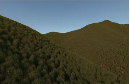
3.5 Downward solar radiation in complex rugged terrain... 44
3.6 Atmosphere simulation... 45
3.7 Concluding remarks ... 46
Chapter 4 Hybrid scene structuring for accelerating 3D radiative transfer ... 47
4.1 Research context ... 49
4.2 Uniform grid in DART ... 50
4.3 Hybrid scene structuring ... 52
4.3.1 Voxel-level ray tracking ... 52
4.3.2 Within-voxel ray tracking... 54
4.3.3 Implementation... 54
4.4 Radiation tracking ... 56
4.5 Experiments... 59
4.5.1 BASEL city scene ... 59
4.5.2 RAMI forest scene ... 60
4.6 Results and Discussion... 61
4.7 Concluding remarks ... 63
Chapter 5 Physical interpretation of leaf area index from LiDAR data ... 65
5.1 Research context ... 67
5.2 Theoretical background... 69
5.2.1 LiDAR pulse ... 69
TABLE OF CONTENTS
5.2.3 DART workflow of point cloud modeling ... 72
5.3 Review of the methods in LPI estimation ... 73
5.3.1 Point number based (PNB) methods ... 74
5.3.2 Intensity based (IB) methods... 75
5.4 Comparative study of LPI/LAI estimation approaches using DART ... 76
5.4.1 Homogeneous scene ... 77
5.4.2 Heterogeneous scene ... 78
5.5 Results and analyses... 79
5.5.1 Homogeneous scene ... 79
5.5.2 Heterogeneous scene ... 84
5.6 Influences of varied leaf dimensions... 87
5.7 Influences of instrumental detection threshold ... 89
5.8 Further discussion and perspectives ... 91
5.9 Concluding remarks ... 94
Chapter 6 Voxel-based reconstruction and simulation of 3D forest scene ... 95
6.1 Research context ... 96
6.2 Study area and material ... 98
6.2.1 Study area... 98
6.2.2 ALS and TLS dataset... 98
6.2.3 Optical dataset ... 99
6.3 Voxel-based 3D PVD inversion ... 99
6.3.1 Single voxel PVD... 99
6.3.2 Incident energy at each return ... 100
6.3.3 Ray traversal in voxels ... 102
6.3.4 Accuracy Validation ... 104
6.3.5 Discussion ... 109
6.4 3D forest scene reconstruction and simulation ... 112
6.4.1 3D landscape reconstruction ... 112
6.4.2 Spectral image simulation and comparison... 113
6.5 Concluding remarks ... 116
Chapter 7 Conclusions and perspectives... 117
7.1 Major conclusions ... 118
LIST OF FIGURES
List of Figures
Figure 1.1: Modeling and inversion scheme in remote sensing. ... 3
Figure 2.1: Framework architecture of LESS... 11
Figure 2.2: ray-tracing process. ... 12
Figure 2.3: Forest described with triangle mesh in LESS. ... 13
Figure 2.4: Storage of triangle mesh in LESS... 14
Figure 2.5: Acceleration structure for the ray-object intersection. ... 15
Figure 2.6: Complex forest with many single trees... 15
Figure 2.7: Forward photon tracing... 17
Figure 2.8: Unit hemisphere partition. The hemisphere is projected onto the horizontal plane as a disk using equal area projection. ... 18
Figure 2.9: Virtual photon approach to calculate BRF. ... 19
Figure 2.10: Scattering calculation in backward path tracing. ... 21
Figure 2.11: Backward path tracing and multiple scattering calculation. ... 22
Figure 2.12: Thermal infrared image simulation using backward path tracing... 23
Figure 2.13: Solar radiation in rugged terrain. ... 24
Figure 2.14: Structures of plane parallel atmosphere. ... 25
Figure 2.15: Radiative transfer in participant media. ... 26
Figure 2.16: Simulating radiative transfer in atmosphere with backward path tracing... 28
Figure 2.17: Free path sampling in plane parallel atmosphere... 29
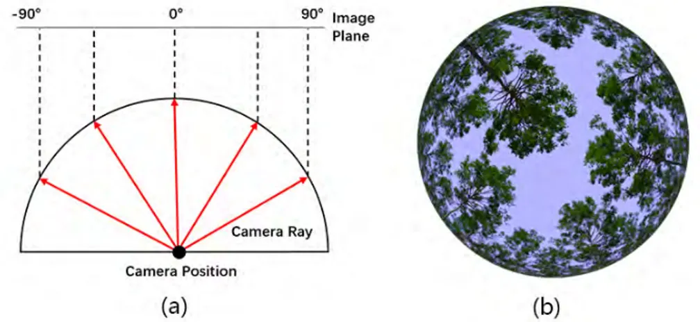
Figure 2.18: Implementation of a circular fisheye camera. (a) The projection diagram of a circular fisheye camera; (b) An example of simulated fisheye image using LESS. ... 30
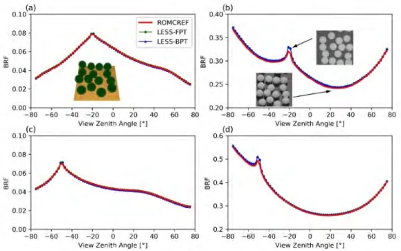
Figure 3.1: Comparison of LESS and RAMI BRFs for a discrete floating sphere scene. ... 35
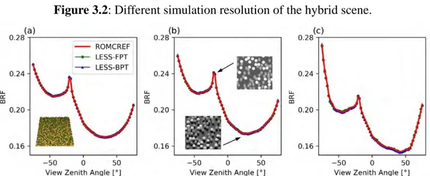
Figure 3.2: Different simulation resolution of the hybrid scene. ... 36
Figure 3.3: Comparison of LESS and RAMI BRFs for a hybrid spherical and cylindrical scene. ... 36
Figure 3.4: Comparison with field measurements and RAPID model. (a) red, principal plane;
... 38
Figure 3.5: Scene description of HET09_JBS_SUM. ... 39
Figure 3.6: Pixel-wise comparison between LESS and DART. ... 40
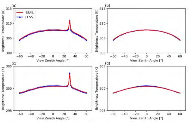
Figure 3.7: Comparison of simulated directional BTs over homogeneous scenes... 41
Figure 3.8: Optical properties of crops and ground: (a) Winter wheat;(b) Corn. ... 43
Figure 3.9: 3D display of the winter wheat and corn: (a) Winter wheat; (b) Corn. ... 43
Figure 3.10: Simulated FPAR and field-measured FPAR profiles. ... 43
Figure 3.11: The study area for downward solar radiation validation... 44
Figure 3.12: Downward solar radiation validation with field measurements. ... 45
Figure 3.13: Downward direct solar radiation and atmosphere radiation. ... 46
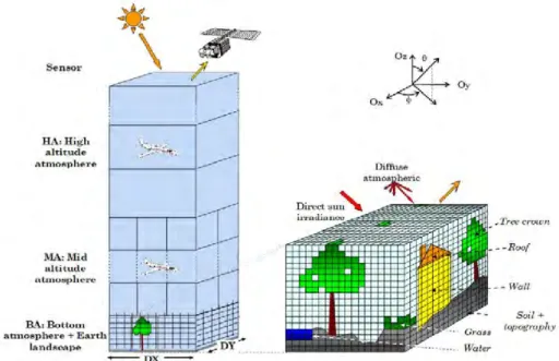
Figure 4.1: Radiative transfer modeling in the “Earth-Atmosphere” scene of DART. The scene of DART is divided into two parts: Earth and Atmosphere... 51
Figure 4.2: Space subdivision and data structure. ... 52
Figure 4.3: The proposed hybrid scene structuring scheme. ... 53
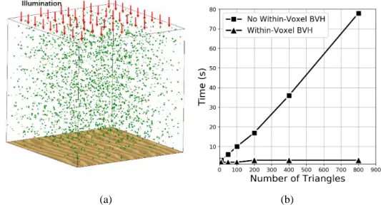
Figure 4.4: Simulation time varies with the number of triangles in one voxel. ... 54
Figure 4.5: Radiation tracking in non-empty voxels. ... 58
Figure 4.6: The BASEL scene under different voxel resolution. ... 60
Figure 4.7: The tree positions and 3D structures of the RAMI forest scene. ... 61
Figure 4.8: Accuracy comparison of the hybrid and uniform approaches when simulating RS images of Basel at three spatial resolutions: 1 m (a), 0.5 m (b) and 0.25 m (c)... 61
Figure 4.9: Accuracy comparison of the hybrid and uniform approaches when simulating RS images of RAMI forest scene at three spatial resolutions: 0.5m (a), 0.25m (b) and 0.1 (c). ... 62
Figure 5.1: Workflow of DART outputs: discrete points in text format or discrete points with associated waveforms in LAS format. ... 72
Figure 5.2: Illustration of 3D Homogeneous test scene ... 78
Figure 5.3: The heterogeneous scene. It is made of randomly distributed trees with ellipsoidal and conical crowns. ... 79
Figure 5.4: LPI estimated by different methods with various LAI and footprint diameter.. 82
Figure 5.5: Average discrete returns for all pulses. ... 82
Figure 5.6: The relationship between LiDAR derived LPI and Reference LPI. ... 83
Figure 5.7: Reference LAI plotted against lnLPI-1... 84
Figure 5.8: Reference LAI plotted against lnLPI-1 for a scene with discrete tree crowns.... 87
1.1 MOTIVATION
... 89
Figure 5.10: LPI estimated by different methods with filtered point cloud ... 90
Figure 5.11: Average discrete returns after filtering for the homogeneous scene. ... 90
Figure 5.12: Reference LAI plotted against lnLPI-1 for heterogeneous scene after filtering. ... 91
Figure 6.1: Voxel PVD inversion using pulse transmittance... 100
Figure 6.2: Incident energy calculation for all echoes in a pulse. ... 102
Figure 6.3: Ray traversal in voxels... 104
Figure 6.4: Comparison between estimated PVD and reference PVD... 105
Figure 6.5: Voxel-based 3D distribution of PVD. ... 106
Figure 6.6: 2D profile of the PAD distribution and its corresponding LiDAR measurements. ... 107
Figure 6.7: Comparison of PAD map with established method. ... 107
Figure 6.8: An illustration of the alignment between ALS and TLS data ... 108
Figure 6.9: 3D voxel of plot L9: (a) ALS; (b) TLS; (c) Vertical profile of the PVD ... 109
Figure 6.10: Top of view of the horizontal PAI distribution for bottom (0-10 m), middle (10– 20 m) and top (20–30 m) layers. The PAI is integrated vertically in each layer for each column. ... 109
Figure 6.11: Number of pulses traverse the voxel... 110
Figure 6.12: Distance between the vegetation-ground pulse to the nearest pure-ground pulse (a) and intensity distribution of pure-ground pulses (b)... 111
Figure 6.13: Standard deviation of intensity in each pixel with different resolutions... 111
Figure 6.14: Base voxels with different LVD... 112
Figure 6.15: Reconstruction of a 100 m×100 m subplot scene from LiDAR point cloud. 113 Figure 6.16: Comparison between LESS simulated image and the field-measured (AISA) hyperspectral image... 115
Figure 6.17: Differences between LESS simulated image and AISA image in a resolution of 25 m... 115
List of Tables
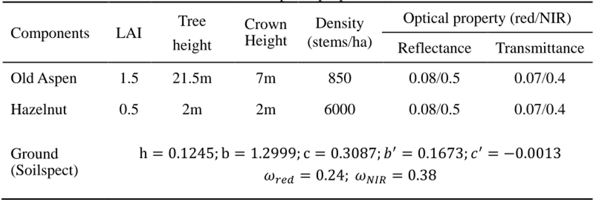
Table 3.1: Structural and optical properties of the OA forest site. ... 37
Table 3.2: Optical properties of landscape elements ... 40
Table 3.3: Computational resources usage (for the resolution of 0.2 m)... 41
Table 3.4: structural properties of winter wheat and corn ... 43
Table 3.5: Parameters for atmosphere simulation... 46
Table 4.1: Computational resources used by simulating BASEL scene... 62
Table 4.2: Computational resources used by simulating RAMI forest scene... 63
Table 5.1: LiDAR parameters used in DART simulations. ... 77
Table 5.2: Fitted parameter c of Eq. (5-23) and R-squared value... 86
LIST OF ACRONYMS
List of Acronyms
ALS Airborne Laser Scanning BOA Bottom of Atmosphere BPT Backward Path Tracing
BRDF Bidirectional Reflectance Distribution Function BRF Bidirectional Reflectance Factor
BSDF Bidirectional Scattering Distribution Function BT Brightness Temperature
BTDF Bidirectional Transmittance Distribution Function BVH Bounding Volume Hierarchy
CDF Cumulative Distribution Function CSF Cloth Simulation Filter
DART Discrete Anisotropic Tadiative Transfer DSR Downward Solar Radiation
FPAR Photosynthetically Active Radiation FPT Forward Photon Tracing
GD Gaussian Decomposition GUI Graphic User Interface ICP Iterative Closest Point IN Intensity Based
LAD Leaf Angle Distribution LAI Leaf Area Index
LiDAR Light Detection and Ranging LOD Leaf Orientation Distribution LPI Laser Penetration Index LUT Look Up Table
LVD Leaf Volume Density PAD Plant Aarea Density PAI Plant Area Density PNB Point Number Based PVD Plant Volume Density
RAMI Radiation Transfer Model Intercomparison RT Radiative Transfer
TLS Terrestrial Laser Scanning TOC Top of Canopy
UEB Urban Energy Budget USR Upward Solar Radiation
Chapter 1. Introduction
Chapter 1
Introduction
Summary
1.1 Motivation... 2 1.2 Scope and objectives ... 4 1.3 Outline of the thesis ... 5
1.1
Motivation
Forests cover approximately 31% of the land surface across the globe and play a prominent role in the global carbon cycle (Mitchard, 2018; Schlamadinger and Marland, 1996; Winjum et al., 1992; Xie et al., 2008). Forests are highly complex and dynamic ecosystems that comprise various species and a large number of individual trees(Arnold et al., 2011; Bass et al., 2001). Besides, forests are an important natural resource, which is widely managed for biodiversity protection, wildlife habitat conservation, forest products and recreation (Twery and Weiskittel, 2013). Therefore, monitoring the status of the forests across the globe has great importance for understanding, utilizing and protecting the forests.
However, human activities (e.g., deforestation) have put great pressure on the environment, which changes the land cover significantly, and then influences the regional and global climatic system. These changes and the resulting effects need to be accessed regionally, as well as globally (Govaerts, 1996).
Currently, satellite remote sensing is the only technology that allows one to monitor large land surface areas with long-term observations. Through the interpretation of satellite observations, we can assess the structure, distribution and functionalities of vegetation canopy either qualitatively or quantitatively. However, optical sensors aboard satellite platforms can only acquire data from a limited number of viewing directions and spectral bands although their signals depend on many factors such as the optical properties of the observed Earth surfaces, the atmosphere, the sensor spectral bands and viewing directions (Zhang et al., 2017), etc. Understanding radiation interaction with the observed Earth surfaces and the atmosphere is essential to retrieve Earth surface information from satellite observation data. For vegetation covers, this understanding is essential for inferring canopy status such as photosynthetically active radiation (PAR).
Through the interpretation of remotely sensed electromagnetic signals (reflected or emitted) to infer the surface status is the “inversion problem” in remote sensing (Figure 1). In general, an inversion procedure is used to determine the input parameters of a model so that model outputs match the available measurements. Ideally, the model is a mathematical relationship. However, due to their complexity, surface structures are usually difficult to be described with simple statistical parameters. It explains why structures are usually simplified in remote sensing models. For example, a one-dimensional (1D) radiative transfer (RT) model simulates a vegetation canopy as horizontal layers with randomly distributed leaves. Based on this simplification, many 1D models, partly derived from atmospheric RT theories, have been established (Kuusk, 2018) to
1.1 MOTIVATION
formulate relationships between bidirectional reflectance factor (BRF) and vegetation parameters (e.g., leaf area index (LAI), leaf angle distribution (LAD), leaf optical properties). Up to now, 1D RT models (e.g., SAIL, SCOPE) have been widely used in remote sensing for parameter retrieval. However, due to their high degree of abstraction of the Earth surfaces, 1D models are usually too inaccurate. For example, they cannot consider the large gaps between crowns and trees with different heights. It explains that three-dimensional (3D) RT models, which can present complex heterogeneous landscapes, are needed for accurate inversion of remote sensing data.
Figure 1.1: Modeling and inversion scheme in remote sensing.
3D RT models use schematic geometric objects (e.g., ellipsoid), triangle mesh and/or voxels with turbid medium to describe 3D scenes. Ray-tracing or radiosity methods are commonly used to solve the RT equation (Disney et al., 2000; Gastellu-Etchegorry et al., 2004; Huang et al., 2013; Qi et al., 2019). They can simulate remote sensing data under arbitrary conditions, which is essential for linking remote sensing signals and realistic surface structures. It allows one to maximally use the information from multi-source remote sensing data and ease the “ill-posed” problem that has confronted remote sensing inversion for many years (Liang et al., 2016).. Nowadays, the potential of 3D RT models increases with the increasing availability of 3D data from various new sensors (e.g., LiDAR: light detection and ranging), provided that 3D RT models can use these 3D data.
However, developing an efficient 3D radiative transfer model that can represent complex 3D landscapes is not an easy task due to the high heterogeneity of the Earth’s surface. To improve efficiency, current models usually work on small realistic scenes or simplify structures with simpler geometries. Although the computer graphics community provides the most accurate and efficient models (known as renderers), they were not designed specifically for performing scientific radiative transfer simulations. Thus, an efficient and adaptable 3D RT model that
works on large-scale and heterogeneous landscapes is important for RT modeling and is highly sought after by the remote sensing community.
Input data of 3D RT models are not always easy to obtain. Usually, realistic canopy structures, instead of simple statistical parameters, are needed. Obtaining detailed vegetation structures
over large areas is also an important aspect for successful canopy modeling works, since 3D structures are the key parameter for 3D radiative transfer model. Due to the high complexity
of vegetation canopies, traditional measurements, such as measuring LAI using LAI-2000, can give very coarse and two-dimensional (2D) parameters only, which is not compatible with 3D RT models. In recent years, LiDAR techniques, which can provide directly canopy 3D information, have been widely used to retrieve forest parameters and reconstruct 3D virtual scenes (Ackermann, 1999; Bailey and Mahaffee, 2017; Bailey and Ochoa, 2018; Bremer et al., 2017; Calders et al., 2018; Côté et al., 2009; Hancock et al., 2017; Müller-Linow et al., 2015; Qi et al., 2016). This is also one of the major topics of this thesis.
1.2
Scope and objectives
A number of problems associated to canopy RT modeling must be solved. “How to build an efficient 3D RT model that can handle large-scale forest landscapes? How to design the RT model to make it easily adaptable to various kinds of remote sensing data? How to validate the RT model? How can complex forest canopy be parameterized and input into the 3D RT model? What are the most effective parameters of the model?” etc. This thesis brings answers to these questions. For that, the objective has been 1) to develop a ray-tracing based 3D RT model (LESS: (LargE-Scale remote sensing data and image Simulation framework) that takes full advantage of the most advanced light transport algorithms of the computer graphics community and 2) to propose a voxel-based canopy parameterization scheme by using airborne LiDAR data.
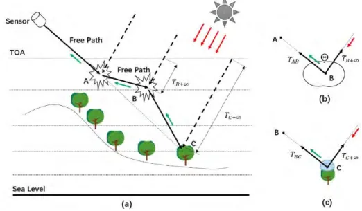
For the development of 3D RT model, this thesis makes full use of the forward and backward ray-tracing modes to simulate different remote sensing data. Specifically, a forward photon tracing (FPT) is proposed to simulate bidirectional reflectance factor (BRF) and energy-balanced related data, e.g., downward and upward solar radiation (DSR/USR) in rugged terrain and incident fraction of photosynthetically active radiation (FPAR). In this mode, a virtual photon approach is used to accelerate BRF simulation with fewer photons. The backward path tracing (BPT) is used for simulating images; it only simulates the energy that exactly goes into the sensor, which saves
1.3 OUTLINE OF THE THESIS
a lot of computation time. The BPT is also extended to simulate thermal infrared images with given temperature distribution and to simulate the RT of a plane-parallel atmosphere.
For the 3D canopy parameterization, we first studied the estimation of laser penetration index (LPI)/leaf area index (LAI) by using simulated airborne LiDAR data from the DART model (Discrete Anisotropic Radiative Transfer). In a first step, DART was accelerated with a specifically designed hybrid scene structure scheme, in order to speed up the simulation of multiple pulse LiDAR over large areas with many vegetation elements. The designed acceleration approach makes it possible to do sensitivity analysis with many DART simulations. It relies on two complementary methods: (1) removal of empty voxels from DART’s regular grids, using a bounding volume hierarchy (BVH), and (2) acceleration of ray-triangle intersection. Using the DART simulated dataset, we quantitatively analyzed several LPI/LAI estimation methods and found that the intensity-based method is the most appropriate one, which is then used to estimate 3D leaf volume density (LVD). Finally, the estimated LVD is used to construct a forest scene and is input into the proposed 3D RT model (LESS) to simulate spectral images.
1.3
Outline of the thesis
Based on the objectives of this thesis, the chapters are organized as follows:
The first chapter introduces the fundamentals of the ray-tracing based 3D RT LESS model. The forward photon tracing and backward path tracing are presented. These modes were extended for simulating DSR/USR, FPAR and thermal infrared radiation. The use of the backward path tracing is also used for simulating RT in a plane-parallel atmosphere.
Chapter 2 is focused on the accuracy of LESS products. Because field BRF data are difficult to obtain, the major validation scheme is cross-validation with other RT models for the case of a few heterogeneous canopies from the RAMI model inter-comparison experiment (
http://rami-benchmark.jrc.ec.europa.eu/HTML/). The RAMI web site stores a few vegetation scenes and
reference BRF values of these scenes. Because the RAMI web site does not store BRF images, the validation of LESS images is done with DART images of a realistic and complex forest scene. LESS FPAR and DSR are validated with field measurements. For atmosphere, LESS is compared to DART and MODTRAN (http://modtran.spectral.com/).
Chapter 3 presents a hybrid scene structuring scheme that was designed in order to accelerate DART. For that, the uniform grid approach of DART is replaced by an efficient data structure. The improvement is shown for a city and a forest scene, both simulated with many small triangles.
Chapter 4 assesses several LPI/LAI inversion approaches, using the optimized DART model with a homogeneous and a heterogeneous canopy. The modeling approach and the implementation that convert full waveform data to discrete points are detailed.
Chapter 5 introduces a voxel-based 3D forest scene reconstruction approach. It utilizes the inverted 3D LVD (cf. chapter 4) and the LESS model (cf. chapter 1). The comparison between LESS and airborne hyperspectral images of 1km forest scene are presented.
Chapter 6 concludes the thesis by summarizing the major conclusions and pointing out perspectives and issues for further researches.
The relationships between the above chapters are visualized in Figure 2.
Chapter 2. LESS: Ray-tracing based 3D radiative transfer model
Chapter 2
LESS: Ray-tracing based 3D radiative
transfer model
Summary
2.1 Research context ... 8 2.2 General framework of LESS... 10 2.3 Fundamentals of ray-tracing ... 11 2.4 3D scene description of LESS ... 13 2.4.1 Geometrical description of 3D scene ... 13 2.4.2 Ray intersection with 3D scene... 14 2.5 Forward photon tracing ... 16 2.5.1 Real photon tracing algorithm... 16 2.5.2 Virtual photon tracing algorithm... 18 2.6 Backward path tracing ... 19 2.6.1 First-order scattering ... 20 2.6.2 Multiple scattering ... 21 2.7 Thermal infrared image simulation... 22 2.8 Downward solar radiation simulation in rugged terrain ... 23 2.9 Atmosphere simulation with backward path tracing... 24 2.9.1 Plane-parallel atmosphere model ... 24 2.9.2 Radiative transfer in participating media ... 25 2.9.3 Radiative transfer in plane-parallel atmosphere... 27 2.10 Implementation and extension of LESS... 29 2.11 Concluding remarks ... 31
This chapter describes the ray-tracing based 3D RT model LESS (LargE-Scale remote sensing data and image Simulation framework) that I developed. This model employs 2 methods. (1) A forward photon tracing method to simulate multispectral bidirectional reflectance factor (BRF) or radiative budget (e.g., downward solar radiation). Photons are weighted simulate more accurate BRF with fewer photons. (2) A backward path tracing method to generate sensor images (e.g., fisheye images) or large-scale (e.g. 1 km2) spectral images. It has been extended to simulate thermal infrared radiation by using an on-the-fly computation of the sunlit and shaded scene components. By extracting information from the photon trajectory, several kinds of remote sensing data, such as the fraction of photosynthetically active radiation (FPAR) and upward/downward radiation over rugged terrain, are simulated. Besides, the backward path tracing has been adapted to simulate atmosphere RT, which enables LESS to simulate a broad range of remote sensing datasets that can be used as benchmarks for various remote sensing applications (forestry, photogrammetry, etc.).
The chapter is presented in the paper:
“Qi, J., Xie, D., Yin, T., Yan, G., Gastellu-Etchegorry, J.-P., Li, L., Zhang, W., Mu, X., Norford, L.K., 2019. LESS: LargE-Scale remote sensing data and image simulation framework over heterogeneous 3D scenes. Remote Sensing of Environment 221, 695–706.”
2.1
Research context
Several 3D RT models that work with rather realistic landscapes were designed during the past decades (Kuusk, 2018). Although they differ from each other significantly, their algorithms are usually classified into two approaches for solving RT equations: (i) Radiosity; (ii) Ray tracing. Radiosity methods, e.g., DIANA (Goel et al., 1991), RGM (Qin and Gerstl, 2000) and RAPID (Huang et al., 2013), are adapted from thermal engineering. Surfaces are usually assumed to be lambertian and the outgoing radiation of each surface is equal to the sum of reflected, transmitted and emitted radiation. This equilibrium can be represented with an equation set, the solution of which gives the radiation distribution of the 3D scene. Borel et al. (1994) is one of the major contributors who applies the radiosity method to vegetation canopy modeling. The core of the radiosity method is to compute a “view factor” between any two scattering surfaces and to store it into a matrix that reaches an unmanageable dimension if the number of surfaces grows very large. To solve this problem, Huang et al. (2013) proposed the RAPID model, which uses porous objects
2.1 RESEARCH CONTEXT
to represent tree crowns. This model enables RAPID to simulate large-scale landscapes. Although the view factor matrix computation is not very efficient, a major advantage of radiosity models is that BRF computation is very fast once the view factor matrix has been computed.
Ray tracing methods are more commonly used in 3D RT models, since they are more adaptive and scalable to complex scenes with many elements (Disney et al., 2000). Depending on objectives, ray tracing methods are implemented in “forward” or “backward” mode. In the forward mode, photons are traced from illumination sources to viewing directions, while backward mode traces rays from the sensor along the viewing direction to determine the 1st, 2nd, etc. scattering order points that contribute to the sensor. Forward mode is more suitable for calculating multi-angle BRFs simultaneously and radiative budget. For example, the DART model is entirely implemented in the forward mode (Gastellu-Etchegorry et al., 2015). Radiation is tracked along discretized directions (i.e, discrete ordinate method) and is collected if it leaves the simulated scene, which enables DART to simulate many products, such as BRF, radiative budget and photosynthetically active radiation (PAR), fluorescence, etc. Forward ray tracing is also used by Raytran (Govaerts and Verstraete, 1998), Rayspread (Widlowski et al., 2006), FLiES (Kobayashi and Iwabuchi, 2008) and FLIGHT (North, 1996). Raytran is a pure Monte-Carlo based model, which traces monochromic rays from light sources. In Raytran, virtual detectors collect rays above the scene and the BRF is estimated by the number of collected rays. Because it does not use any weighting mechanism (i.e., a ray is totally scattered or absorbed), the implementation of this model is relatively straightforward. However, it also makes Raytran less efficient, because many rays are usually necessary to produce a convergent result. When calculating BRF, the rays absorbed within the scene do not contribute to the detector, which is a waste of computation time. Besides, absorption and reflectance are wavelength dependent. Therefore, simulating multiband BRF is generally computationally intensive as new rays must be sent separately per band. The Rayspread model is an extension of Raytran as it introduces a secondary ray mechanism, which traces a series of rays towards the detector at each intersection point of the main photon trajectory. This approach saves a lot of time when calculating BRF because it uses a much smaller number of photons. To simulate multispectral data more efficiently, the librat model (Lewis, 1999) uses a “ray bundle” concept to simulate multiband BRF in a single ray path by updating the weight for each band according to the reflectance/transmittance at each intersected point.
However, despite its advantage in simulating multiple directional BRFs in a single simulation, forward tracing is usually less efficient in simulating a particular sensor image, mostly due to the tracking of energy that ultimately does not contribute to the simulated image. The efficiency is
The weakness of the forward mode, however, is the strength of the backward mode, since backward ray tracing traces only the rays that enter the sensor. It allows one to simulate sensor images of very large scenes with many landscape elements. DIRSIG (Goodenough and Brown, 2012) is a typical representative of this kind of model, using backward path tracing to estimate surface-leaving radiance. This makes DIRSIG very efficient for performing hardware design and evaluating sensor configurations. Therefore, the ability to simulate remotely sensed signals in both forward and backward modes is an important feature for a modern and adaptive RT model.
The algorithms described above (i.e., radiosity and ray tracing) are classically used in computer graphics, especially for image rendering. In the computer graphics community, open-source renderers such as PBRT (Pharr et al., 2016) and POV-Ray (Plachetka, 1998) have been developed for handling 3D scenes and tracing rays to find intersections, using optimized techniques such as the advanced acceleration data structures (e.g., bounding volume hierarchy (Mller and Fellner, 2000)) and the CPU-level optimizations (Purcell and Hanrahan, 2004) (e.g., Streaming SIMD Extensions 2 [SSE2]). However, these renderers are not universally applicable, because they are mostly focused on image rendering for human perception rather than on radiometric accuracy for scientific applications. For example, they usually work only with three broad spectral bands (RGB) or a few fixed spectral bands in the visible region, which is not adapted to hyperspectral data simulations. Developing novel remote sensing-specific models based on these renderers or reimplementation is a pragmatic solution. For instance, Auer et al. (2016) developed a 3D SAR simulator based on POV-Ray, which can simulate radar reflection effects of 3D objects. Recently, DIRSIG has been re-designed and re-implemented, to adopt the latest advances of light transport algorithms emerged in the computer graphics community (Goodenough and Brown, 2017). DART model has integrated the ray tracing engine Embree (Wald et al., 2014), which is a collection of high-performance ray tracing kernels, to accelerate RT simulations.
2.2
General framework of LESS
The design of an operational 3D RT model requires numerous developments such as 3D scene description, illumination conditions, sensor configurations and RT modeling (Disney et al., 2000). A framework that considers all these aspects is an ideal tool to give accessibility to 3D RT simulation for most users. The LESS modeling framework has 6 major modules (Figure 2.1): Input Data Management module. It manages all the input parameters, including 3D landscape
2.3 FUNDAMENTALS OF RAY-TRACING
of Python scripts for efficient input of parameters. Landscape elements in LESS are represented with geometric primitives (e.g., ellipsoid and cylinders) or triangle meshes. They are usually created by third-party software, such as Onyx Tree.
3D Landscape Construction module. It includes several sub-processors to convert different types of data into a format that the RT Model module can use. For example, the sub-module Terrain Processor converts the DEM (digital elevation model) image into a triangle mesh or a height field. Usually, a height field is more efficient in terms of computation time and memory than a triangle mesh (Tevs et al., 2008). The sub-module Optical Data Processor calculates the reflectance and transmittance of different landscape elements by interpolating spectra of the spectral database (provided by LESS or imported by users), according to the user-defined bands. Visualization module. It is intended for 2D and 3D displays of the simulated landscape. It helps
users to interactively explore the created scene and allows them to verify the correctness of the constructed 3D landscape before the actual computation.
RT Model module. It is the key module of the LESS framework. It uses a parallelized ray tracing method to simulate the interaction between the solar radiation and landscape elements based on the previously constructed 3D scene and the sensor configuration. It contains several RT models, e.g., forward photon tracing and backward path tracing, to meet different simulation purposes. Parallel Computing module. It offers the ability to run LESS on a Local Server or a Cluster,
which enables LESS to simulate large-scale areas.
Products Processing module. It contains tools to post-process LESS outputs. For example, radiance images, combined with sun / sky irradiance, can be converted into BRF images.
Figure 2.1: Framework architecture of LESS.
2.3
Fundamentals of ray-tracing
In computer graphics, ray-tracing is a rendering technique that generates 2D images from 3D scenes by sending rays and simulating their physical interactions with virtual objects. The radiance
leaving a point 𝑞𝑞 in direction 𝜔𝜔𝑜𝑜 can be expressed with a rendering equation (Kajiya, 1986): 𝐿𝐿𝑜𝑜(𝑞𝑞, 𝜔𝜔𝑜𝑜) = 𝐿𝐿𝑒𝑒(𝑞𝑞, 𝜔𝜔𝑜𝑜) + � 𝑓𝑓(𝑞𝑞, 𝜔𝜔𝑖𝑖, 𝜔𝜔𝑜𝑜)
4𝜋𝜋 𝐿𝐿𝑖𝑖(𝑞𝑞, 𝜔𝜔𝑖𝑖)|cos 𝜃𝜃𝑖𝑖|𝑑𝑑𝜔𝜔𝑖𝑖
(2-1) where 𝐿𝐿𝑜𝑜(𝑞𝑞, 𝜔𝜔𝑜𝑜) is the outgoing radiance from point 𝑞𝑞 along direction 𝜔𝜔𝑜𝑜; 𝑓𝑓(𝑞𝑞, 𝜔𝜔𝑖𝑖, 𝜔𝜔𝑜𝑜) is the Bidirectional Scattering Distribution Function (BSDF) of the intersected surface, which determines the outgoing radiance along direction 𝜔𝜔𝑜𝑜 at point 𝑞𝑞 induced by incoming radiance along incident direction 𝜔𝜔𝑖𝑖 ; 𝐿𝐿𝑖𝑖(𝑞𝑞, 𝜔𝜔𝑖𝑖) is the incoming radiance; 𝜃𝜃𝑖𝑖 is the angle between 𝜔𝜔𝑖𝑖 and the surface normal and 𝐿𝐿𝑒𝑒(𝑞𝑞, 𝜔𝜔𝑜𝑜) is an emission term (e.g., thermal emission). In short, the outgoing radiance is the sum of emitted and scattered radiance (Figure 2.2).
A complete ray-tracing process usually includes the following steps:
Geometrical description of the 3D scene. The structures of the 3D scene should be explicitly expressed. Landscape elements are usually represented with geometric objects, triangle meshes and voxels with turbid media.
Generation of rays. Rays are generated from light sources and propagate into the virtual scene. The sun and atmosphere are typical light sources. Some ray-tracing techniques send rays from sensors instead of light sources, which is more commonly used for simulating images only. Intersection test between ray and scene. Intersection test is the core of ray-tracing and also
the most time-consuming process, since a scene may contain millions of elements and testing each ray for each element is impractical. To improve efficiency, some acceleration techniques are used, such as the bound volume hierarchy (BVH).
Radiance calculation. By recording the energy change at each intersection point, the radiance recorded by sensors can be known explicitly. Besides, the ray trajectory also provides the possibilities to query other information, e.g., FPAR.
2.4 3D SCENE DESCRIPTION OF LESS
2.4
3D scene description of LESS
2.4.1 Geometrical description of 3D scene
An accurate description of the 3D scene is the fundamental step for conducting reliable radiative transfer simulations. Generally, geometric objects are expressed with math equations, which could ease the ray-object intersection by solving analytic equations. However, it is usually used to represent some simple elements only, such as tree crowns. FLIGHT model (North, 1996) is a typical 3D model that uses geometric objects filled with turbid media to simulate 3D scenes. The concept “turbid medium” is from atmospheric science, but the difference is that turbid medium in remote sensing of vegetation is described with a group of parameters that are related to canopies, e.g., leaf volume density (LVD), LAD, leaf reflectance and transmittance.
Compared to geometric objects and turbid medium, a triangle mesh is more appropriate to accurately describe complex and heterogeneous vegetation canopies, since realistic canopies cannot be simply represented by statistical parameters. Triangle mesh uses millions of small triangles to represent the object’s surfaces. Usually, the more the number of triangles is bigger and the better the representation of the original object, but it needs more computational resources.
LESS uses triangle mesh as its major scene description scheme for obtaining very accurate simulations. Figure 2.3 shows a complex forest with more than 10 million triangles. It appears that each single leaf is composed of several small triangles in order to simulate complex leaf shapes.
Figure 2.3: Forest described with triangle mesh in LESS.
triangle, which means that 3N vertices need to be stored if N triangles exist. It results in redundant information, since one vertex may belong to several triangles. A more efficient way is to store all vertices in an array, and to store the vertex indices of each triangle in another array. Hence, vertices XYZ are stored in a vertex array and vertex indices are stored in an index array (Figure 2.4).
Figure 2.4: Storage of triangle mesh in LESS.
2.4.2 Ray intersection with 3D scene
A 3D scene may contain hundreds and thousands of objects, and each object may be composed of millions of small triangles. To find the intersection point of an incident ray, the intersected small triangle should first be found. The naive implementation is to test all the triangles in the scene one by one, which gives a time complexity of O(n).
However, an incident ray may be intersected with objects that are close to its trajectory only. Triangles far from the raypath can be safely removed from the list of possible intersecting triangles. This selection / removal approach can be achieved with the so-called object bounding box. A bounding box is simply a cube that tightly surrounds the object (Figure 2.5). If a ray does not intersect with the bounding box, it does not intersect the object itself, and there is no need to test a possible intersection. Since the ray-box intersection is usually much efficient than ray-object intersection, this method can efficiently find the intersected object.
Despite the high efficiency of ray-box intersection, we still do not want to test all object bounding boxes with a ray one by one, especially for scenes with a large number of objects. Usually, an acceleration structure is used here to skip some boxes, which has been widely used in computer graphics, such as KD-Tree and BVH. For each intersected object, if it contains too many triangles, a second level of acceleration structure is usually used. Now, the basic unit is a single triangle.
2.4 3D SCENE DESCRIPTION OF LESS
Figure 2.5: Acceleration structure for the ray-object intersection.
Let us consider a complex forest with many single trees, each one having many triangles. In
Figure 2.6, the forest scene has more than 100,000 single trees, and each tree has more than 1
million triangles. If the triangle vertices are represented with float number, the memory used by this scene may exceed 1000 GB, which is impossible for most common computers. To handle this kind of situation, an “instancing” technique is commonly used. This method only stores several single trees in memory, and then “clones” them to different places by storing the transform matrix only for each instanced tree. Since the single tree is not actually copied, this method saves a lot of computer memory and time for copying data. Unfortunately, this approach is not adapted for simulating 3D radiative budget, at least per triangle.
2.5
Forward photon tracing
2.5.1 Real photon tracing algorithm
Forward photon tracing (FPT) traces photon packets with the power 𝑃𝑃(𝜆𝜆) into the scene from light sources. The initial power 𝑃𝑃0(𝜆𝜆) of each packet is determined by the power of light sources and the number 𝑁𝑁 of generated packets. When generating photon packet in a scene with multiple light sources, a light source is randomly chosen according to the importance weight 𝑤𝑤𝑘𝑘, which is proportional to the power of each light source, i.e., 𝑤𝑤𝑘𝑘 = ∑ 𝐿𝐿𝑘𝑘(𝜆𝜆)
𝐿𝐿𝑘𝑘(𝜆𝜆) 𝐾𝐾
𝑘𝑘=1 with 𝐿𝐿𝑘𝑘(𝜆𝜆) being the power of light source 𝑘𝑘 and 𝐾𝐾 being the number of light sources. This mechanism guarantees that a light source with larger power has more sampled photon packets. The initial power of each packet, in terms of watt (W), is given as
𝑃𝑃0(𝜆𝜆) =∑𝐾𝐾𝑘𝑘=1𝐿𝐿𝑘𝑘(𝜆𝜆)
𝑁𝑁 (2-2)
When a photon packet enters the scene along a path defined by its origin and direction of propagation, the occurrence of an intersection with landscape elements is tested. If an intersection occurs, the power of this packet is scaled according to the optical properties of the intersected surface, i.e., the reflectance or transmittance. For a packet with 𝑄𝑄 times of scattering before it escapes from the scene, the power becomes:
𝑃𝑃𝑄𝑄(𝜆𝜆) = 𝑃𝑃0(𝜆𝜆) ∙ ��𝜋𝜋𝑓𝑓(𝑞𝑞, 𝜔𝜔
𝑖𝑖,𝜔𝜔𝑜𝑜,𝜆𝜆)/𝑝𝑝𝑞𝑞� 𝑄𝑄
𝑞𝑞=1
(2-3) where 𝑓𝑓(𝑞𝑞, 𝜔𝜔𝑖𝑖,𝜔𝜔𝑜𝑜,𝜆𝜆) is the bidirectional scattering distribution function (BSDF) at the 𝑞𝑞th intersection point during its trajectory. 𝜔𝜔𝑖𝑖 and 𝜔𝜔𝑜𝑜 are the incident and outgoing directions of a photon packet, respectively. 𝑝𝑝𝑞𝑞 is the probability that the photon is reflected or transmitted (e.g., 0.5). Since in LESS, surfaces are Lambertian, the BSDF is the bidirectional reflectance distribution function (BRDF) or bidirectional transmittance distribution function (BTDF), depending on relative configurations of 𝜔𝜔𝑖𝑖,, surface normal 𝜔𝜔𝑛𝑛 and 𝜔𝜔𝑜𝑜.
𝑓𝑓(𝑞𝑞, 𝜔𝜔𝑖𝑖, 𝜔𝜔𝑜𝑜, 𝜆𝜆) =𝜋𝜋 �1 𝜌𝜌𝜌𝜌⊥,𝜆𝜆∙ sgn(𝜔𝜔𝑛𝑛∙ 𝜔𝜔𝑖𝑖) + 𝜏𝜏𝜆𝜆∙ sgn(−𝜔𝜔𝑛𝑛 ∙ 𝜔𝜔𝑖𝑖) if 𝜔𝜔𝑜𝑜∙ 𝜔𝜔𝑛𝑛 ≥ 0
⊤,𝜆𝜆∙ sgn(−𝜔𝜔𝑛𝑛 ∙ 𝜔𝜔𝑖𝑖) + 𝜏𝜏𝜆𝜆 ∙ sgn(𝜔𝜔𝑛𝑛 ∙ 𝜔𝜔𝑖𝑖) if 𝜔𝜔𝑜𝑜∙ 𝜔𝜔𝑛𝑛 < 0 (2-4)
where sgn(𝑥𝑥) = �1, x ≥ 0
0, x < 0; 𝜌𝜌⊥,𝜆𝜆𝜋𝜋 and 𝜌𝜌⊤,𝜆𝜆
𝜋𝜋 are the upper and bottom surface BRDF, respectively; 𝜏𝜏𝜆𝜆
2.5 FORWARD PHOTON TRACING
side are assumed to be identical. The outgoing direction of a photon packet after scattering is determined by randomly sampling the BSDF function. For Lambertian surfaces, the model chooses a random direction in the outgoing hemisphere. Since a single photon trajectory can be used to simulate BRF for any wavelength by updating the power according to the spectral reflectance/transmittance, for simplicity, the symbol 𝜆𝜆 is omitted below.
A photon packet is collected by the sensor if it exits the scene through the scene top boundary. Lateral boundary effects are considered to simulate horizontally infinite scenes with a repetitive pattern. As shown in Figure 2.7, the photon packet which exits from the lateral boundaries will re-enter the scene from the opposite side with the same photon direction until it escapes through the top boundary of the scene. When the scattering order of a packet exceeds an user-defined threshold (e.g., 5), the propagation of the packet is randomly stopped according to the “Russian roulette” mechanism (Kobayashi and Iwabuchi, 2008), which terminates the trajectory of a packet with a probability 𝑝𝑝 (e.g., 5%). If the packet survives, its power will be multiplied by 1
1−𝑝𝑝.
Figure 2.7: Forward photon tracing.
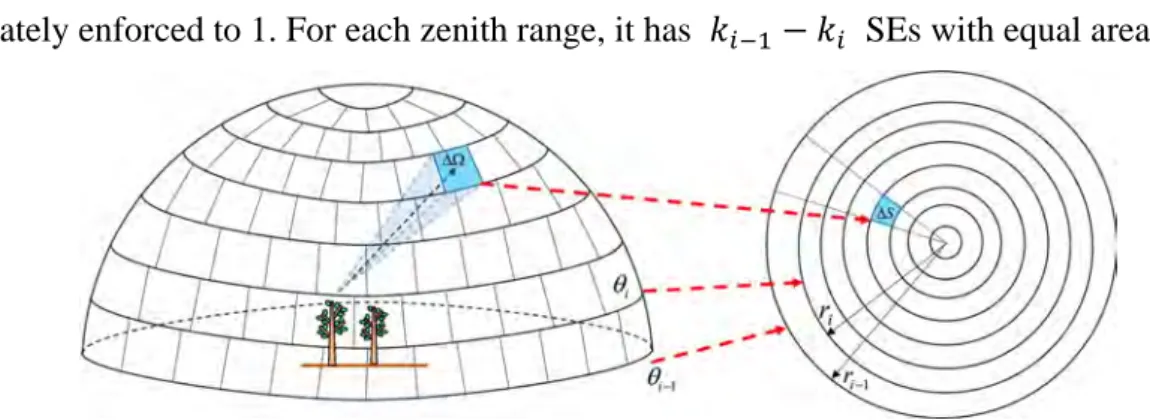
The collection of the escaped photon packets is achieved by placing a virtual hemisphere above the scene (Govaerts and Verstraete, 1998). The hemisphere (Figure 2.8) is partitioned into 𝑁𝑁𝑃𝑃 surface elements (SE) with equal area 𝛥𝛥𝛥𝛥 = 2𝜋𝜋𝑁𝑁𝑃𝑃, using the partition scheme of a disk via the
equal area projection (i.e., ∆𝛺𝛺 = 𝛥𝛥𝛥𝛥). Zenith angles are defined (Beckers and Beckers, 2012) with: 𝜃𝜃𝑖𝑖 = 𝜃𝜃𝑖𝑖−1−𝑎𝑎 2 𝑎𝑎𝑎𝑎𝑝𝑝𝑒𝑒𝑎𝑎𝑎𝑎sin 𝜃𝜃𝑖𝑖−1 2 � 𝜋𝜋 𝑘𝑘𝑖𝑖−1, 𝑘𝑘𝑖𝑖 = 𝑘𝑘𝑖𝑖−1� 𝑟𝑟𝑖𝑖 𝑟𝑟𝑖𝑖−1� 2 (2-5)
where (𝜃𝜃𝑖𝑖, 𝜃𝜃𝑖𝑖−1) defines a zenith range on the hemisphere with 𝜃𝜃0 =𝜋𝜋
2; 𝑘𝑘𝑖𝑖 is the total number of
SEs for a zenith angle 𝜃𝜃𝑖𝑖 with 𝑘𝑘0 = 𝑁𝑁𝑃𝑃; 𝑟𝑟𝑖𝑖 is the radius corresponding to 𝜃𝜃𝑖𝑖 with 𝑟𝑟𝑖𝑖 = 2 sin𝜃𝜃𝑖𝑖
2
approximately enforced to 1. For each zenith range, it has 𝑘𝑘𝑖𝑖−1− 𝑘𝑘𝑖𝑖 SEs with equal area.
Figure 2.8: Unit hemisphere partition. The hemisphere is projected onto the horizontal plane as a disk using
equal area projection.
When a photon packet exits the scene, the outgoing SE (solid angle) is determined by the photon direction only, i.e., the hemisphere is placed at an infinite position. The BRF in this SE can be estimated with (Govaerts and Verstraete, 1998):
𝑓𝑓𝐵𝐵𝐵𝐵𝐵𝐵𝑖𝑖 =
𝜋𝜋𝑃𝑃𝑖𝑖𝐴𝐴
∆𝛺𝛺𝑖𝑖 ∙ cos 𝜃𝜃𝑖𝑖𝑎𝑎 ∙ 𝑃𝑃𝑎𝑎𝑎𝑎𝑒𝑒𝑛𝑛𝑒𝑒
(2-6)
where 𝑃𝑃𝑖𝑖𝐴𝐴 is the power (watt) of all the captured photons in SE 𝑖𝑖, i.e., 𝑃𝑃𝑖𝑖𝐴𝐴 = ∑𝑃𝑃𝑄𝑄∈∆𝛺𝛺𝑖𝑖𝑃𝑃𝑄𝑄; ∆𝛺𝛺𝑖𝑖 =
2𝜋𝜋
𝑁𝑁𝑃𝑃 is the solid angle of each SE; 𝜃𝜃𝑖𝑖
𝑎𝑎 is the central zenith angle of solid angle ∆𝛺𝛺
𝑖𝑖; 𝑃𝑃𝑎𝑎𝑎𝑎𝑒𝑒𝑛𝑛𝑒𝑒 is the
power of all the direct incident photon packets on a reference plane at the top of the scene, i.e., the incident radiation at the top of the scene. Once the power in each SE is determined, the scene albedo is computed as:
𝜔𝜔𝑎𝑎𝑎𝑎𝑎𝑎𝑒𝑒𝑎𝑎𝑜𝑜 =∑ 𝑃𝑃𝑖𝑖 𝐴𝐴 𝑁𝑁𝑃𝑃 𝑖𝑖=1 𝑃𝑃𝑎𝑎𝑎𝑎𝑒𝑒𝑛𝑛𝑒𝑒 (2-7)
2.5.2 Virtual photon tracing algorithm
The real photon approach estimates BRF by using small SEs on the sphere. More photon packets are needed to reduce the variance when smaller SEs are used. To solve this problem, a virtual photon approach, similar to the virtual direction in DART model (Yin et al., 2015), secondary ray in Rayspread model (Widlowski et al., 2006) or some “local estimates” methods (Antyufeev and Marshak, 1990; Marchuk et al., 1980), is introduced. If a packet is intercepted by an object (e.g., a tree) in the scene without complete absorption, the packet will be scattered in a direction which is randomly sampled by the BSDF function, and a virtual photon packet will be
2.6 BACKWARD PATH TRACING
sent to each of the defined virtual directions. The possible scattered energy, in terms of intensity (W ∙ sr−1), is calculated as
𝐼𝐼 = 𝑉𝑉 ∙ 𝑃𝑃𝑞𝑞−1∙ 𝑓𝑓(𝑞𝑞, 𝜔𝜔
𝑖𝑖, 𝜔𝜔𝑣𝑣) ∙ cos < 𝜔𝜔𝑣𝑣, 𝜔𝜔𝑛𝑛 > (2-8)
where 𝑃𝑃𝑞𝑞−1 is the power of the incident photon packet at the 𝑞𝑞th intersection point along its trajectory; 𝜔𝜔𝑣𝑣 is a virtual direction; 𝑉𝑉 is a visibility factor that is equal to zero if a landscape element occludes the virtual photon packet, and equal to 1 otherwise. When sending the occlusion testing rays, the lateral boundary effect is also considered (Figure 2.9). The final BRF is then:
𝑓𝑓𝐵𝐵𝐵𝐵𝐵𝐵𝑣𝑣 =
𝜋𝜋𝐼𝐼𝑣𝑣𝐴𝐴
cos 𝜃𝜃𝑣𝑣∙ 𝑃𝑃𝑎𝑎𝑎𝑎𝑒𝑒𝑛𝑛𝑒𝑒
(2-9) where 𝐼𝐼𝑣𝑣𝐴𝐴 is the power per unit solid angle (W ∙ sr−1) in virtual direction 𝑣𝑣 and 𝜃𝜃𝑣𝑣 is the zenith angle of the virtual direction. An advantage of calculating a directional BRF using the virtual photon approach is that the BRF is estimated for an infinitely small solid angle (Thompson and Goel, 1998), which is the real directional BRF of a scene.
Figure 2.9: Virtual photon approach to calculate BRF.
2.6
Backward path tracing
Instead of tracing photon packets from light sources, backward path tracing sends rays from sensors into the scene. The ray directions are controlled by sensor configurations (field of view, position, orientation, etc.). The main task of this ray-tracing algorithm is to establish a connection, which is called “path”, between light sources and sensors and to determine the radiance incident onto the sensor.