IMPACT OF ALGORITHM, ITERATIONS, POST-SMOOTHING, COUNT LEVEL AND TRACER DISTRIBUTION ON SINGLE-FRAME POSITRON EMISSION TOMOGRAPHY QUANTIFICATION USING A GENERALIZED
IMAGE SPACE RECONSTRUCTION ALGORITHM
by
Étienne Létourneau, Medical Physics, McGill University, Montreal
April 2012
A thesis submitted to McGill University in partial fulfillment of the requirements for the degree of:
Master of Sciences in Medical Physics
3
REMERCIEMENTS
Je désire remercier toutes les personnes qui ont contribué à la réalisation de cette thèse, que ce soit par leur aide directe au projet ou par leur soutien.
Je remercie tout d’abord Andrew J. Reader, mon directeur de recherche, pour ses nombreux encouragements, sa confiance, sa capacité à me motiver, ses précieux conseils et son dévouement. Je remercie également Jeroen Verhaeghe pour son aide inestimable avec qui j’ai appris beaucoup, Paul Gravel pour les discussions et sa bonne humeur contagieuse ainsi que Pawel Markiewicz pour son aide.
Je tiens également à souligner le soutien du personnel du programme de Physique Médicale de l’université McGill en commençant par Margery Knewstubb pour son travail exceptionnel et pour les nombreuses matinées à être la première à me saluer dans le département. Les professeurs : Jan Seuntjens et Ervin B. Podgorsak pour leur passion et leurs conseils bons pour la vie, François DeBlois pour l’opportunité de recherche, Issam El-Naqa pour les discussions passionnantes, William Parker pour sa motivation, Slobodan Devic pour être qui il est, John Kildea pour la qualité de son enseignement, Gabriela Stroian pour avoir été capable de transformer de longues séances de laboratoire les soirs de semaine en moments agréables, Pierre Léger pour sa dévotion et Michael Evans pour les discussions ainsi que pour les beignets.
Ces deux années n’auraient pas eu la même saveur sans la présence des autres étudiants du programme, soit Martin, Desmond, Avery, Laurie, Amanda, Rafael, James, Allison, Pete, Vincent, Sergei et Hamed sans oublier Eunah pour son aide. Merci pour votre amitié et votre solidarité, je me suis senti privilégié de faire partie de ce groupe.
Un merci spécial aux personnes qui m’ont transmis la passion pour les sciences : Ronald Redmond sans qui je n’aurais pas choisi cette voie, Bernard Marcheterre pour son partage du plaisir de l’enseignement et Viktor Zacek pour m’avoir donné ma première chance dans le milieu de la recherche universitaire, pour sa gentillesse et ses innombrables lettres de référence! À toute ma famille, pour leur soutien et leur amour.
4
ACKNOWLEDGEMENTS
I would like to thank everyone who contributed to the realization of this thesis, whether it is for their direct help to the project or by their moral support.
Firstly, thanks to my research director, Andrew J. Reader for his cheering, his trust in me, his capacity to motivate, his precious advices and his dedication to duty. I’m also thankful to Jeroen Verhaeghe for his invaluable help with whom I learned a lot, to Paul Gravel for the discussions and his cheerfulness and to Pawel Markiewicz for his help. The support of the McGill University Medical Physics team is also worthy of notice starting with Margery Knewstubb for her exceptional work and for the plentiful mornings at the department being the first to greet me. The professors: Jan Seuntjens and Ervin B. Podgorsak for their passion and their lifetime advices, François DeBlois for his research opportunity, Issam El-Naqa for the fascinating talks, William Parker for his cheering up, Slobodan Devic for being who he is, John Kildea for the quality of his teaching, Gabriela Stroian for being able to turn a long lab session during the evening into an enjoyable moment, Pierre Léger for his devotion and Michael Evans for the discussions and the donuts.
These two years wouldn’t have been the same without the presence of the other students in the program, that are Martin, Desmond, Avery, Laurie, Amanda, Rafael, James, Allison, Pete, Vincent, Sergei and Hamed without forgetting Eunah Chung for her help. Thanks for your friendship and solidarity, I feel blessed to be part of this group.
A very special thanks for those who passed me the passion for science: Ronald Redmond without whom I wouldn’t have choose the path of physics, Benard Marcheterre for sharing the joy of teaching and Viktor Zacek for giving me my first occasion to do research during my undergrad, for his kindness and his countless reference letters!
5
RÉSUMÉ
La tomographie par Émission de Positons est une technique d’imagerie médicale traçant les procédures fonctionnelles qui se déroulent dans le patient. L’une des applications courantes de cet appareil consiste à performer un diagnostique subjectif à partir des images obtenues. Cependant, l’imagerie quantitative (IQ) permet de performer une analyse objective en plus de nous procurer de l’information additionnelle telle que la courbe temps-activité (CTA) ainsi que des détails visuels qui échappent à l’œil. Le but de ce travail était, en comparant plusieurs algorithmes de reconstruction tels que le ML-EM PSF, le ISRA PSF et les algorithmes qui en découlent ainsi que la rétroprojection filtrée pour une image bidimensionnelle fixe, de développer une analyse robuste sur les performances quantitatives dépendamment de la localisation des régions d’intérêt (RdI), de leur taille, du niveau de bruit dans l’image, de la distribution de l’activité et des paramètres post-lissage. En simulant des acquisitions à partir d’une coupe axiale d’un cerveau digitale sur Matlab, une comparaison quantitative appuyée de figures qualitative en guise d’outils explicatifs a été effectuée pour toutes les techniques de reconstruction à l’aide de l’Erreur Absolue Moyenne (EAM) et de la relation Biais-Variance. Les résultats obtenus démontrent que la performance de chaque algorithme dépend principalement du nombre d’événements enregistré provenant de la RdI ainsi que de la combinaison itération/post-lissage utilisée qui, lorsque choisie adéquatement, permet à la majorité des algorithmes étudiés de donner des quantités similaires dans la majorité des cas. Parmi les 10 techniques analysées, 3 se sont démarquées : ML-EM PSF, ISRA PSF en utilisant les valeurs prévues avec lissage comme facteur de pondération et RPF avec un post-lissage adéquat les principaux prétendants pour atteindre l’EMA minimale.
Mots-clés: Tomographie par émission de positons, Maximum-Likelihood Expectation-Maximization, Image Space Reconstruction Algorithm, Rétroprojection Filtrée, Erreur Absolue Moyenne, Imagerie quantitative.
6
ABSTRACT
Positron Emission Tomography (PET) is a medical imaging technique tracing the functional processes inside a subject. One of the common applications of this device is to perform a subjective diagnostic from the images. However, quantitative imaging (QI) allows one to perform an objective analysis as well as providing extra information such as the time activity curves (TAC) and visual details that the eye can’t see. The aim of this work was to, by comparing several reconstruction algorithms such as the MLEM PSF, ISRA PSF and its related algorithms and FBP for single-frame imaging, to develop a robust analysis on the quantitative performance depending on the region of interest (ROI), the size of the ROI, the noise level, the activity distribution and the post-smoothing parameters. By simulating an acquisition using a 2-D digital axial brain phantom on Matlab, comparison has been done on a quantitative point of view helped by visual figures as explanatory tools for all the techniques using the Mean Absolute Error (MAE) and the Bias-Variance relation. Results show that the performance of each algorithm depends mainly on the number of counts coming from the ROI and the iteration/post-smoothing combination that, when adequately chosen, allows nearly every algorithms to give similar quantitative results in most cases. Among the 10 analysed techniques, 3 distinguished themselves: ML-EM PSF, ISRA PSF with the smoothed expected data as weight and the FBP with an adequate post-smoothing were the main contenders for achieving the lowest MAE.
Keywords: Positron Emission Tomography, Maximum-Likelihood Expectation-Maximization, Image Space Reconstruction Algorithm, Filtered Backprojection, Mean Absolute Error, Quantitative Imaging.
7
TABLE OF CONTENTS
REMERCIEMENTS ... 3 ACKNOWLEDGEMENTS ... 4 RÉSUMÉ ... 5 ABSTRACT ... 6 FIGURES ... 9 INTRODUCTION ... 12 THEORY ... 15 Physical principles ... 15 Electron-positron anihilation ... 15 Detection principle ... 16 Sinograms ... 17PET detection system ... 17
PET exam and radiopharmaceuticals of interest ... 18
Fluorodeoxyglucose (18F) ... 18 Pittsburgh compound B (11C) ... 18 Raclopride (11C) ... 18 Mathematical principles ... 18 Poisson process ... 18 Signal-to-noise ratio ... 19 Derivation ... 19 ML-EM ... 22 ISRA ... 22
General ISRA with any linear combination as weight. ... 22
FBP ... 23
Evaluation metrics ... 25
THE EXPERIMENT ... 26
RESULTS ... 31
FDG – Homogeneous ground truth ... 31
PiB and Raclopride – Homogeneous ground truth ... 43
8 CONCLUSION AND SUMMARY ... 58 REFERENCES ... 59 APPENDIX A ... 65
9
FIGURES
Figure 1 : Different types of coincidences. ... 16 Figure 2 : Relation between object and sinogram space. ... 17 Figure 3 : Visualisation of the objective function and the derivative of the objective function as a function of the expected image... 20 Figure 4 : Projection of a LoR parallel to axis l at a distance s from the middle of the detector and at angle φ.. ... 23 Figure 5 : Slide 140 of the original 3D brain phantom from Rahmim et al. (2008). ... 27 Figure 6 : Relevant ROIs The basal ganglia (bottom right) are composed of the nucleus caudatus, the putamen and the pallidum. ... 27 Figure 7 : The corresponding colors and the signs of the reconstruction algorithms. ... 31 Figure 8 : Homogeneous ground truth for FDG with inverse color. ... 31 Figure 9 : MAE as a function of iteration for the homogeneous ground truth of FDG distribution with different mean counts. ... 33 Figure 10 : MAE as a function of iteration for the homogeneous ground truth of FDG distribution with different ROIs. ... 35 Figure 11 : Qualitative images of the bias for the homogeneous ground truth of a FDG distribution. Positive bias is in red, negative in blue and neutral in black. Both images were obtained with MLEM PSF when the MAE in the white matter had a minimal value. The mean counts are a) 11.7k and b) 389.3k for the transverse plane of interest. ... 35 Figure 12 : Bias-Variance relation in white matter for homogeneous ground truth of FDG distribution. ... 37 Figure 13 : MAE as a function of iteration for the homogeneous ground truth of FDG distribution with different ROI sizes. ... 38 Figure 14 : Lowest MAE achieved as a function of mean counts for the homogeneous ground truth of the FDG distribution in frontal lobe ... 40 Figure 15 : MAE as a function of iteration and count level without post-smoothing
(except c) FBP) for the homogeneous ground truth of the frontal lobe. ... 41 Figure 16 : MAE as a function of iteration for homogeneous ground truth of: a) FDG, b) PiB, c) Raclopride in the full white matter ... 44 Figure 17 : Lowest MAE achieved as a function of mean counts for the homogeneous ground truth of the PiB distribution in frontal lobe ... 46 Figure 18 : Qualitative images of the bias for the homogeneous ground truth of a PiB distribution. ... 47 Figure 19 : Lowest MAE achieved as a function of mean counts for the homogeneous ground truth of the Raclopride distribution in frontal lobe ... 48 Figure 20 : Qualitative images of the bias for the homogeneous ground truth of a
Raclopride distribution... 49 Figure 21 : MAE as a function of iteration for a central pixel of the frontal lobe for a FDG distribution ... 56
10
Figure 22 : Lowest MAE achieved as a function of mean counts for different
11
TABLES
Table 1 : Characteristics of common positron emitters in PET imaging. ... 15 Table 2 : Relative activity distributions based on commonly used radiopharmaceuticals. ... 28 Table 3 : Different levels of heterogeneity as ground truth for FDG distributions. ... 29 Table 4 : Qualitative grid of the expected image giving the lowest MAE in the full frontal lobe using post-smoothing as a function of counts for all the techniques. ... 43 Table 5 : Reconstruction algorithms achieving the lowest MAE using post-smoothing as a function of counts for every ROI, ROI size and radiopharmaceutical with a homogeneous ground truth. ... 54
12
INTRODUCTION
The previous years in medical imaging were characterized by a shift from a subjective observer–dependent diagnostic and prognostic to an objective quantitative analysis. In fact, organizations such as the Quantitative Imaging Biomarkers Alliance (QIBA) by the Radiological Society of North America (RSNA) promote and favour the clinical implementation of quantitative imaging that will reduce the variance across hardware and software platforms. According to them, quantitative imaging is:
“the extraction of quantifiable features from medical images for the assessment of normal or the severity, degree of change, or status of a disease, injury, or chronic condition relative to normal. Quantitative imaging includes the development, standardization, and optimization of anatomical, functional, and molecular imaging acquisition protocols, data analyses, display methods, and reporting structures. These features permit the validation of accurately and precisely obtained image-derived metrics with anatomically and physiologically relevant parameters, including treatment response and outcome, and the use of such metrics in research and patient care."
A good application of quantitative imaging in neurology using Positron Emission Tomography (PET) would improve diagnostic and management of common diseases such as Alzheimer’s disease (AD), Parkinson’s disease (PD), frontotemporal dementia (FTD) as well as brain tumors and other neurological disorders. From an anatomical perspective, the development of these diseases occurs in well-known regions of the brain. For example, the β-amyloid plaque deposition which is one of the fundamental causes of Alzheimer’s disease starts in the hippocampus before propagating to the temporal lobe and the frontal lobe or, likewise, the lack of dopamine in the basal ganglia which is typically associated with Parkinson’s disease. In such cases, task-oriented QI could be used to compare the different patterns between normal and cancerous or affected regions of interest, hence the importance of a good selection of the reconstruction algorithm. Because quantitative analysis when performed manually can be time-consuming and consequently not convenient for clinical purposes, standardization of QI methods is the logical way to benefit from the advantages of QI without introducing negative aspects.
13
Previous important publications in order to increase image quality already proposed several iterative reconstruction methods such as the weighted least-squares, the algebraic reconstruction technique, the space-alternating generalized expectation-maximization algorithm, the maximum-a-posteriori estimation and the median root prior to name a few amongst others. Some studies are also evaluating the effects of post-smoothing on different techniques and to the best knowledge of the author of this document, no previous work has been presenting a detailed study on post-smoothing effects for common reconstruction algorithms with realistic clinical activity distributions. Over that, most studies deal with a single number of counts and an application of post-smoothing at a unique point during the reconstruction.
Within the framework of this single frame imaging research project, a general iterative equation has been derived from the weighted least-squares objective function from which, with the appropriate choice of weight was obtained the classical case of ML-EM, the image space reconstruction algorithm (ISRA) and the weighted ISRA with the weight being any linear combination of the measured and expected data, smoothed or not. Filtered back-projection (FBP) was the only analytical method considered. The statistical measures used are the average level bias-variance relation and the average pixel-level mean absolute error (MAE) given as a percentage. The experiment was done using simulated brain data with these particular aspects that distinguish this work from previous research:
10 different reconstruction algorithms were considered
3 different radiopharmaceutical activity distributions corresponding to common clinical cases with 2 heterogeneous ground truths for the FDG based on transverse brain phantom (A. Rahmim et al., 2008).
10 different count levels covering a realistic range with a special consideration for low counts that can be often encountered in practice.
A task-oriented analysis on 6 different regions of interest which are of interest to neuroscientists and in addition, 3 different ROI sizes are considered.
14
Once all the iterations are done, post-smoothing over all the images for each iteration was applied until the lowest MAE value was reached. This way, the optimal iteration/post-smoothing combination was obtained.
Note that these simulations constitute a significant extension of our previous work (Reader, A.J, Letourneau, E., Verhaeghe, J. (2011)) where it had already been shown that for an arbitrary activity distribution with homogeneous ROIs, ML-EM with point spread function (PSF) and FBP weren’t always giving the lowest MAE. Results appeared to be ROI and ROI size dependent. No post-smoothing was considered at that stage except for FBP.
15
THEORY
Physical principles
Electron-positron annihilation The general beta plus (β+
) decay is represented by:
(1)
Z, the atomic number, is equal to the number of protons. A is the atomic mass number equal to the number of nucleons in the corresponding atom (i.e. the sum of protons and neutrons). P represents the Parent atom and D the Daughter, e+ is a positron (i.e. electron antiparticle: same mass as an electron but with a positive charge instead) and υe is a neutrino.
Table 1 : Characteristics of common positron emitters in PET imaging.
The average range of the positron into organ tissues is about 1 to 3 mm before annihilating with an electron generating 2 gamma rays of about 511 keV going in opposite directions.
(2)
Because the momentum of both particles (positron and electron) might not be nil when they annihilate together, the angle between them can be slightly different than 180˚ and the energy over 511 keV for both photons, resulting in a resolution decrease.
Radionuclides Nuclear reaction Half-life (min) Max. positron energy (MeV) Mean positron range in water (mm) Carbon-11 14N(p,α)11C 20.38 0.96 1.1 Nitrogen-13 16O(p,α)13N 9.97 1.19 1.4 Oxygen-15 14N(d,n)15O 2.03 1.70 1.5 Fluorine-18 18O(p,n)18F 109.77 0.64 1.0
16
Detection principle
The PET scanner role is to detect photons in coincidences (i.e. detected within the same time window with two different detectors). The line linking the two detectors that triggered is called the line of response (LoR) and an acquisition involves collecting events along these LoRs. As represented in figure 1, there are 3 different kinds of coincidences.
Figure 1 : Different types of coincidences.
The true event occurs when gamma rays from the same annihilation are detected without any of them being scattered nor absorbed. The scatter event occurs when gamma rays from the same annihilation are detected when one or both had been scattered before reaching detector which creates a false LoR. The random event occurs when gamma rays from different annihilations are detected within a short time range which creates a false LoR. The ratio of these three types of coincidences depends on the stopping power, the energy resolution, the attenuating object and the coincidence timing window.
17
Sinograms
Figure 2 : Relation between object and sinogram space.
Each LoR is represented by a distance from the middle of the detector (s) and an angle ( ) between the projection and the vertical axis. For a given point in space, if there is a large number of counts, a sinusoidal shape will appear as show on figure 2. The further the point of annihilation is from the middle of the detector, the more amplified the sinusoidal shape will be (i.e. a point perfectly in the middle of the detector would result into a vertical line in the sinogram space).
PET detection system
The detection of a 511 keV photon arising from positron emitters is accomplished using a combination of solid scintillation detectors and photomultiplier tubes (PMT). The solid detector absorbs radiation and then, after a certain amount of time (in the order of nanoseconds) called the scintillation decay time, emits flashes of light. These photons are converted to an electrical pulse by the PMT, amplified and finally sorted by a pulse height analyzer (PHA) before being registered as a count if the corresponding energy of the interacting γ-ray wasn’t discriminated by the PHA and both photons were detected within a coincidence time window. The choice of the detector depends on its stopping power (proportional to the crystal thickness), the scintillation decay time (efficiency at high count rate), and the light output (energy resolution).
18
PET exam and radiopharmaceuticals of interest
Radiopharmaceuticals are molecules to which a radioactive isotope (see table 1) has been incorporated. Each radiopharmaceutical aims to a specific biological process. For this reason, PET is a functional and not an anatomical imaging method that will vary depending on the molecule employed.
Fluorodeoxyglucose (18F)
The 18F –FDG targets regions with a high glucose concentration such as heart, kidneys, brain and cancerous cells. The half-life of the fluorine-18 isotope is of 109.77 minutes and it is relatively easy to synthesise which makes it the most commonly used radiopharmaceutical in PET imaging. By studying the reduction of glucose metabolism in several brain regions such as the hippocampus, the temporal lobe, the parietal lobe and the frontal lobe, diagnostic of frequent pathologies like Alzheimer’s disease (AD), frontotemporal “Pick’s” dementia (FTD), vascular dementia, epilepsy and Huntington’s disease to name just a few can be achieved.
Pittsburgh compound B (11C)
The 11C-PiB is an analog of thioflavin use to scan the beta-amyloid (Aβ) plaques deposition in the brain which is the fundamental cause for Alzheimer’s disease. PiB-PET is relevant for diagnostic and also for giving the probability of developing this disease. The half-life of carbon-11 is 20.38 minutes.
Raclopride (11C)
It is an antagonist binding to the neurotransmitter dopamine receptor D2. By competing with dopamine mainly in the basal ganglia area, raclopride can give an indication of the neuronal degeneration which is typical aspect of the Parkinson’s disease.
Mathematical principles
Poisson process
A popular and a reasonable way to represent the PET emission process for each bin i is the Poisson distribution
19
(3)
where m and q are the measured and expected data respectively. However, factors in processing the raw signal might change pixel values to non-Poisson behaviour and in some cases pre-correction for random coincidences would also result in a non-Poisson distribution. Nevertheless, the Poisson distribution is still a good and simple approach to work with in quantitative imaging.
Signal-to-noise ratio
The signal-to-noise ratio (SNR) is an indicator of the level of desirable signal to the level of background noise:
(4)
where μ is the mean and σ is the standard deviation. For the case of a Poisson distribution in a PET acquisition, the standard deviation is equal to the square root of the mean which results in:
(5)
where N is the mean number of counts. The equation above can be used to guide the selection of the count levels. The number of counts should not be selected with equal count values between each level but it should follow a square root law in order to have equidistant SNRs and as a consequence, equidistant image quality levels.
Derivation
The starting point is the iterative weighted least-squares objective function
(6) where
20
(7)
is the expected data, j is the image pixel index, i is the sinogram bin index and k is the iteration number. aij is an element of the system-matrix A that tells the contribution of
pixel j into the sinogram bin i. eta represent the scatter and random events. mi is the
measured data and wi(k) is the weight which is considered (at this stage) to be constant at
each iteration.
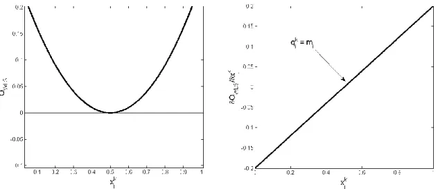
Figure 3 : Visualisation of the objective function and the derivative of the objective function as a
function of the expected image and how to achieve better estimate of xj(k) which are closer to the
minimum of the objective function.
Because an iterative algorithm dictated by the WLS is of interest, the gradient of equation 6 according to xjk can be written:
(8)
According to Figure 3, the objective function is having a minimum meaning that the gradient needs to be subtracted. Then, a general iterative formula could be represented by:
21
(9)
where the step size λj(k), for simplification reasons, is set to:
(10)
From figure 3 above, we can notice that when xj(k) is overestimated, the differential
expression of the WLS function will be positive which will result into a negative shift according to equation 9 and vice versa for underestimated xj(k). Substituting (8) and (10)
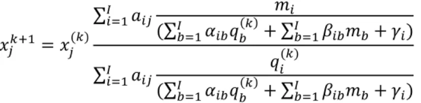
into (9): (11)
The new iterative value of a given pixel is the previous value times a pixel-by-pixel ratio of the backprojection of the weighted measured data over the backprojection of the weighted expected data. This general form (11) contains well-known cases such as ML-EM (Maximum Likelihood Expectation Maximization) and ISRA (Image Space Reconstructed Algorithm) with a proper choice of weight.
22
The advantages of the iterative methods are that we can accurately model the image formation process and include the correction factors (attenuation, scatter, normalization, etc.). The main disadvantages are that it is time consuming and it is hard to predict the behaviour.
ML-EM
We can obtain the ML-EM algorithm by selecting wi(k) being equal to qi(k) :
(12)
The Maximum Likelihood Expectation Maximization algorithm appears to be an iterative update of the measured and expected bin-to-bin data ratio. An alternative derivation of the ML-EM algorithm is available in Appendix A.
ISRA
We can obtain ISRA by selecting wi(k) being equal to 1:
(13)
The Image Space Reconstruction Algorithm appears to be the pixel-by-pixel ratio of the backprojection of the measured over the backprojection of the expected data.
General ISRA with any linear combination as weight. The general expression:
23 (14)
suggests that the weight can be any linear combination of measured and expected data, smoothed or not. γ stands for the offset in order to avoid a division by zero. For example, in the case of α being nil and β being equal to 1 we would get the reconstruction algorithm called M-ISRA:
(15) FBP
The Radon transform is an integral of a distribution over a sum of lines at multiple angles : (16)
Figure 4 : Projection of a LoR parallel to axis l at a distance s from the middle of the detector and at
angle φ. The radon transform is the collection of the projections at different angle φ of the
24
According to figure 4, the delta Dirac function would have a non-zero value only along the LoR (red line) parallel to the l axis at an angle and a distance s from the middle of the detector. is the projection of the LoR that can be represented by a point in the sinogram. The goal of an analytical reconstruction algorithm is to go back directly from all these projections to the spatial distribution.
The Fourier transform of the projection is defined as:
(17) By simply replacing (16) in (17): (18) where (19) (20) Rewriting (21)
The previous steps contained the Central Section Theorem (CST) defined as: The FT of a
projection corresponds to a line of the FT of the image crossing the origin at an angle of
with the abscissa.
(22)
25 (23) (24) Where: (25) (26) (27)
Transforming to polar coordinates:
(28)
(29)
Equation 29 is the filtered backprojection. Note that we can use the absolute value due to the fact that is going from 0 to because of the identity (27). The absolute value is the ramp filter amplifying high frequencies and removing star-burst artefacts. It also compensates for the oversampling in the middle of the Fourier space.
The principal pros and cons of the analytical reconstruction method are that analytical is much faster while it is easier to implement correction factors for the iterative methods.
Evaluation metrics
All the evaluation metrics employed in this project were at the pixel level in order to be in a parametric imaging context. For each metric, P is the number of pixels in the Region of Interest (ROI), N the number of realizations, n the realization number and tj represent
26
value and the reference value. These differences are summed over all the realizations and then averaged over the pixels of the given ROI.
(30)
The pixel variance (31) is the difference between the measured data and the average of the measured data. These differences are squared, summed over the realizations and averaged over the pixels of the given ROI.
(31)
The pixel-level mean absolute error in percentage is the difference between measured and reference values. These differences are in absolute value, normalized by the reference value and summed over the realizations. In order to express this quantity in relative terms, a factor of 100 over the number of pixels multiplies the quantity.
(32)
The pixel-level MAE (%) is the principal evaluation metric employed in this project in order to discriminate between the reconstruction algorithms.
THE EXPERIMENT
For each simulation, a 256 by 256 pixels transverse plane of a 3-D realistic digital brain phantom was used. This plane, from an anatomical point of view, is similar to the well-known Hoffman 2-D brain phantom. The corresponding sinogram space has dimensions of 256 (s-axis) by 288 ( -axis).
27 Figure 5 : Slide 140 of the original 3D brain phantom from Rahmim et al. (2008). The transverse plane was originally a 200 x 200 pixels object but an additional edge of 28 nil pixels was appended in order to have a dimension of 256 by 256 pixels that match with those of the High Resolution Research Tomograph (HRRT).
The full object was split into 6 standardized ROI (figure 6) that represent distinct regions of the brain.
White Matter Thalamus Occipital Lobe
Temporal Lobes Frontal Lobe Basal Ganglia
Figure 6 : Relevant ROIs The basal ganglia (bottom right) are composed of the nucleus caudatus, the putamen and the pallidum.
For each ROI, three different sizes were selected: a) Full ROI as represented in figure 6
28
b) Sub ROI. Similar as the full with an average of 3 pixels taken off from the outline of the ROI. This reduction was performed using the function bwmorph with the argument ‘shrink’ in Matlab.
c) Central pixel ROI. A single pixel is selected randomly away from the edges of the full ROI.
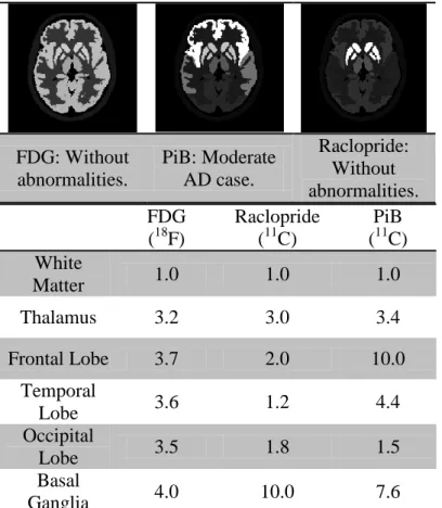
Three typical activities depending on the radiopharmaceutical were designed based on literature review and on true image analysis using the medical imaging software VINCI (“Volume Imaging in Neurological research, Co-registration and ROIs Included”).
FDG: Without abnormalities. PiB: Moderate AD case. Raclopride: Without abnormalities. FDG (18F) Raclopride (11C) PiB (11C) White Matter 1.0 1.0 1.0 Thalamus 3.2 3.0 3.4 Frontal Lobe 3.7 2.0 10.0 Temporal Lobe 3.6 1.2 4.4 Occipital Lobe 3.5 1.8 1.5 Basal Ganglia 4.0 10.0 7.6
Table 2 : Relative activity distributions based on commonly used radiopharmaceuticals. Details on each radiopharmaceutical can be found in the theory section under PET exam and
radiopharmaceuticals of interest
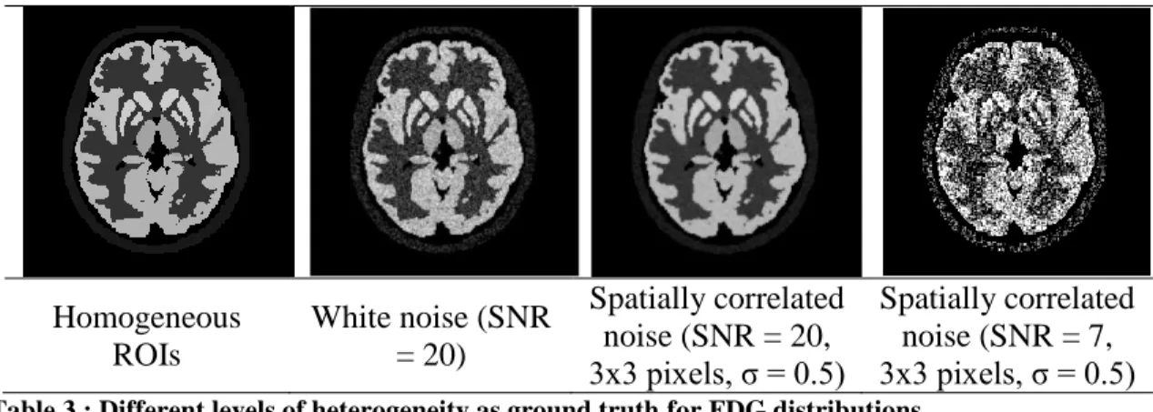
Furthermore, because PET is a functional imaging system showing complex networks of cells and receptors that aren’t homogeneous, four heterogeneity levels were selected according to table 3 as ground truths. Since the real degree of heterogeneity is unknown, both small and high signal-to-noise ratios were selected in order to cover a wide interval in which the real case would probably be.
29 Homogeneous ROIs White noise (SNR = 20) Spatially correlated noise (SNR = 20, 3x3 pixels, σ = 0.5) Spatially correlated noise (SNR = 7, 3x3 pixels, σ = 0.5) Table 3 : Different levels of heterogeneity as ground truth for FDG distributions.
The mean count values were selected based on true images of the ECAT High-Resolution Research Tomograph (HRRT) machine at the Montreal Neurological Institute. Selecting a considerable number of acquisitions using the program VINCI in which the worst and best image qualities were identified, 10 mean count values were selected between these boundaries in such a way that the SNRs would be uniformly represented along an interval going from 1.0k to 350k mean counts for the transverse plane of interest (approximately between 2.0x10⁵ and 5.0x10⁷ counts for the whole 3D volume).The quantitative and qualitative aspects of the reconstructed image in the simulation correlated with the images from real acquisitions. Each simulation considered 100 realizations, 120 iterations and 10 different noise levels. These noise levels correspond to 1.75k, 10.5k, 26.3k, 52.6k, 78.9k, 114k, 158k, 210k, 263k and 389k mean counts per slice for FDG, to 1.32k, 7.93k, 19.8k, 39.6k, 59.5k, 85.9k, 119k, 159k, 198k and 264k counts per slice for PiB and to 0.757k, 4.54k, 11.4k, 22.7k, 34.1k, 49.2k, 68.2k, 90.9k, 114k and 151k counts per slice for Raclopride. Prior to forward projection of the scaled ground truth brain phantom, a Gaussian convolution kernel (σ=1.5, ~3.5 pixels FWHM) was applied to simulate limited system resolution.
The system matrix was taken to be A=XH, where X performs line integrals through an image estimate to deliver sinogram bin values, and H performs a convolution re presenting the point spread function (PSF). The PSF compensates for factors affecting the resolution which are the tilting of the crystal detectors, the non-collinear photons, the positron range and other resolution degrading factors. The system and the reconstruction PSF are represented in the code using a Gaussian function of σ=1.5 (FWHM = 3.53 pixels) and σ=1.275 (FWHM = 3.00 pixels, 85% of the system) pixels respectively which
30
has the effect of reducing the high frequency content of the data. The PSF used in the reconstruction should be slightly narrower than the true point spread response of the system in order to avoid the Gibbs ringing artefact.
Each noisy sinogram at each scaling level was reconstructed by ten different image reconstruction methods: 1) ML-EM (w(k)=q(k)) 2) ML-EM with PSF (w(k)=q(k)) 3) ISRA with PSF (w(k)=1) 4) M-ISRA with PSF (w(k)=m) 5) Q-ISRA with PSF (w(k)=q(k)) 6) (0.5M+0.5Q)-ISRA with PSF (w(k)=0.5m + 0.5q(k))
7) (0.5M+0.5Q, 2S)-ISRA with PSF, using the same sinogram weights as method 6, but with the weights smoothed by a Gaussian convolution kernel (σ=2 pixels) 8) (M, 2S)-ISRA with PSF, using the same sinogram weights as method 4, but with the weights smoothed by a Gaussian convolution kernel (σ =2 pixels) (i.e.
h ih h
k
i m
w() , where the matrix elements {β
ih} correspond to applying a
Gaussian convolution kernel with σ =2 pixels)
9) (Q, 2S)-ISRA with PSF, using the same sinogram weights as method 5, but with the weights smoothed by a Gaussian convolution kernel (σ =2 pixels) (i.e.
h k h ih k i qw() (), where the matrix elements {α
ih} correspond to applying a
Gaussian convolution kernel with σ=2 pixels)
10) Filtered backprojection (FBP), ramp filtered, with post-reconstruction smoothing.
All the ISRA methods employed an offset of 0.05 in order to avoid division by zero. For this reason, MLEM PSF and Q-ISRA PSF are not identical methods. Post-smoothing was done using a 15x15 pixels Gaussian filter with σ of 0.6 pixel (FWHM = 1.41). This filter was applied 60 times at each (un-smoothed) reconstruction iteration for iterative algorithms and 120 times for the analytical algorithm.
31
RESULTS
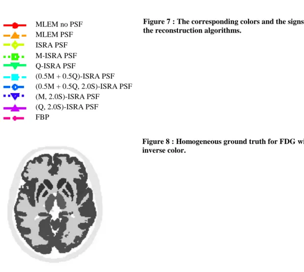
Figure 7 : The corresponding colors and the signs of the reconstruction algorithms.
Figure 8 : Homogeneous ground truth for FDG with inverse color.
Figure 7 is the legend used for all the plots in this section. Also, in order to have neater images to analyse from a qualitative point of view, the colors were inverted as show in Figure 8.
FDG – Homogeneous ground truth
The first simulation was done for the radiopharmaceutical FDG considering a homogeneous ground truth (See Table 2).
MLEM no PSF MLEM PSF ISRA PSF M-ISRA PSF Q-ISRA PSF (0.5M + 0.5Q)-ISRA PSF (0.5M + 0.5Q, 2.0S)-ISRA PSF (M, 2.0S)-ISRA PSF (Q, 2.0S)-ISRA PSF FBP
32 a) b) 20 40 60 80 100 120 50 100 150 200 Iterations M A E ( % )
FDG - Frontal lobe (Full ROI), Mean counts :1947
20 40 60 80 100 120 50 100 150 200 Iterations M A E ( % )
33
c)
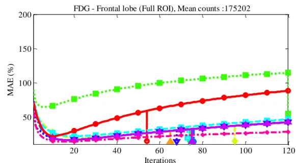
Figure 9 : MAE as a function of iteration for the homogeneous ground truth of FDG distribution with different mean counts.
Figure 9 shows the impact of a modification in the total number of counts on the mean absolute error. The mean count values are only for the transverse slice of interest and not for the whole 3D image. The corresponding legend is shown in Figure 7. The vertical lines correspond to the smallest MAE value obtained using post-smoothing. As expected, as the total number of counts increases contributing to a more consistent measured sinogram, MAE decreases. A shift of the point at which the lowest MAE with and without post-smoothing is achieved can also be noticed. Indeed, as the number of counts increased, the minimum MAEs are achieved at a higher number of iterations. Finally, the ideal iteration number at which post-smoothing should be applied in order to obtain the lowest MAE is always after the iteration number giving the lowest MAE without post-smoothing. 20 40 60 80 100 120 50 100 150 200 Iterations M A E ( % )
34 a) b) c) 20 40 60 80 100 120 20 40 60 80 100 120 140 Iterations M A E ( % )
FDG - Basal ganglia (Full ROI), Mean counts :175202
20 40 60 80 100 120 20 40 60 80 100 120 140 Iterations M A E ( % )
FDG - Frontal lobe (Full ROI), Mean counts :175202
20 40 60 80 100 120 20 40 60 80 100 120 140 Iterations M A E ( % )
35 Figure 10 : MAE as a function of iteration for the homogeneous ground truth of FDG distribution with different ROIs.
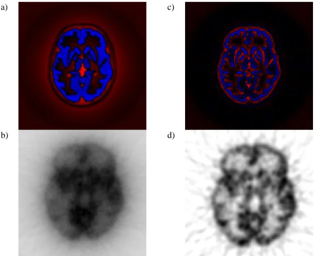
Figure 10 shows the impact of the region of interest on the MAE with the other parameters fixed. Few differences are noticeable especially when comparing white matter with the other ROIs. These differences appeared above all at low iteration numbers. A plausible explanation for such a variation would be to consider the bias in the ROIs. According to Figure 11 a), every ROI except white matter is having a negative bias. Knowing that the activity in the white matter is low (cold spot), this positive bias could be due to the non-negativity constraint of the iterative reconstruction algorithms reducing the standard deviation at the cost of introducing a positive bias.
a) c)
b) d)
Figure 11 : Qualitative images of the bias for the homogeneous ground truth of a FDG distribution. Positive bias is in red, negative in blue and neutral in black. Both images were obtained with MLEM PSF when the MAE in the white matter had a minimal value. The mean counts are 11.7k for a) and b) and 389.3k for c) and d) for the transverse plane of interest.
Parts b) and d) of Figure 11 enable assessment of the impact of count level on image quality and contrast.
36
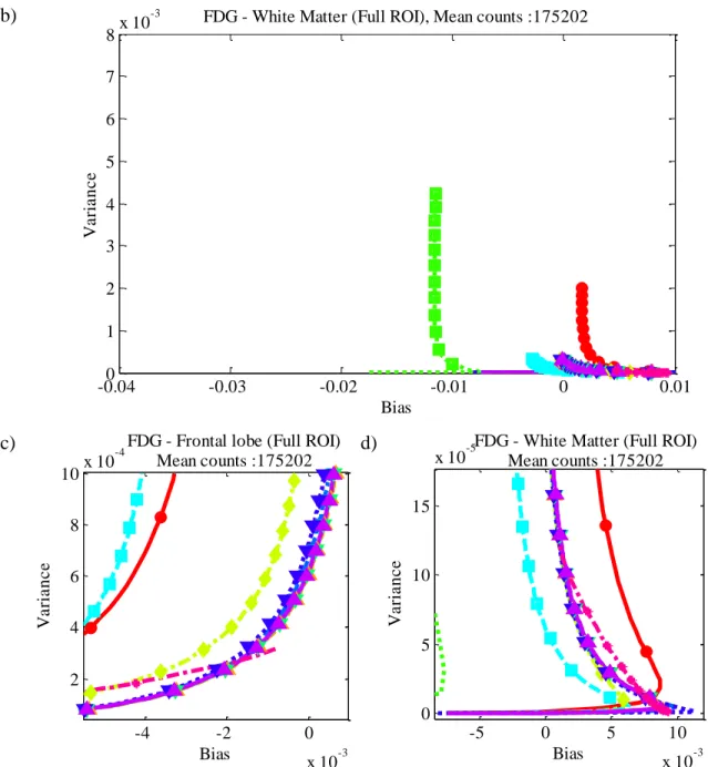
Broadly speaking, as iterations go by, the bias is decreasing while the variance increases as show on Figure 12 a). However, for white matter (Figure 12 b)) it can be observed that at low iteration (below 10) the bias will rapidly increase reaching positive values before decreasing. Because MAE is influenced by both bias and variance, it is a fair assumption to say that the iteration at which MAE is the lowest represents a point on the bias-variance curve being close to the origin. Thus, from Figure 12, it can be seen why the lowest MAE without post-smoothing was achieved sooner in the white matter than in the other ROIs (Figure 10). In practice, no reconstruction stops after such a low number of iterations which make these results misleading from a practical point of view.
a) -0.040 -0.03 -0.02 -0.01 0 0.01 1 2 3 4 5 6 7 8x 10 -3 Bias V a ri a n c e
37
b)
c) d)
Figure 12 : Bias-Variance relation in white matter for homogeneous ground truth of FDG distribution. c) and d) are close-ups of a) and b) respectively.
For the homogeneous ground truth, the effects of changing ROI size are negligible, the reason being that even for a central pixel the surrounding ones have the same ground truth and as a consequence their influence on the pixel of interest isn’t detrimental.
-0.040 -0.03 -0.02 -0.01 0 0.01 1 2 3 4 5 6 7 8x 10 -3 Bias V a ri a n c e
FDG - White Matter (Full ROI), Mean counts :175202
-4 -2 0 x 10-3 2 4 6 8 10x 10 -4 Bias V a ri a n c e
FDG - Frontal lobe (Full ROI) Mean counts :175202 -5 0 5 10 x 10-3 0 5 10 15 x 10-5 Bias V a ri a n c e
FDG - White Matter (Full ROI) Mean counts :175202
38
a)
b)
Figure 13 : MAE as a function of iteration for the homogeneous ground truth of FDG distribution with different ROI sizes.
Figure 14 shows the lowest MAE achieved without (a) and with (b) post-smoothing. Remember that for FBP, the iteration corresponds to repeated applications of the Gaussian smoothing kernel. As expected, all the methods converge to the same MAE as the number of counts increases. Another observation is that, except for M-ISRA PSF and
20 40 60 80 100 120 20 40 60 80 100 120 140 Iterations M A E ( % )
FDG - Frontal lobe (Sub ROI), Mean counts :175202
20 40 60 80 100 120 20 40 60 80 100 120 140 Iterations M A E ( % )
39
(0.5M + 0.5Q)-ISRA PSF, all the reconstruction techniques give almost identical MAE with an adequate combination of iteration number and post-smoothing application. a) b) 0 0.5 1 1.5 2 2.5 3 3.5 4 x 10⁵ 0 20 40 60 80 100 Mean counts L o w e st a c h ie v e d M A E ( % )
FDG - Frontal lobe (Full ROI)
0 0.5 1 1.5 2 2.5 3 3.5 4 x 10⁵ 0 20 40 60 80 100 Mean counts L o w e st P o st -s m o o th M A E a c h ie v e d ( %
40
c) d)
Figure 14 : Lowest MAE achieved as a function of mean counts for the homogeneous ground truth of the FDG distribution in frontal lobe: a) without post-smoothing, b) with post-smoothing, c) without post-smoothing (high noise level close-up), d) with post-smoothing (high noise level close-up).
Figures 14 c) and d) are close-ups on the high noise level portion of a) and b) respectively. It can be noticed that the general order between the methods according to their performance doesn’t change except for MLEM no PSF where post-smoothing application has a similar effect than PSF. Also, an adequate application of post-smoothing can reduce the MAE by more than 10% for a small number of counts.
a) 0.5 1 1.5 2 2.5 3 x 10⁴ 20 30 40 50 60 Mean counts L o w e st a c h ie v e d M A E ( % )
FDG - Frontal lobe (Full ROI)
0.5 1 1.5 2 2.5 3 x 10⁴ 20 30 40 50 60 Mean counts L o w e st P o st -s m o o th M A E a c h ie v e d ( %
41
b)
c)
Figure 15 : MAE as a function of iteration and count level without post-smoothing (except c) FBP) for the homogeneous ground truth of the frontal lobe.
The maps of Figure 15 bring together the information of the different sub-plots of Figure 9. It is also an efficient approach to know how good a reconstruction algorithm is doing and in which cases. For example, M-ISRA PSF would be totally inappropriate for high noise levels.
42 Counts : 1.9k Counts : 29.2k Counts : 87.6k Counts : 175.2k Counts : 292.0k
ML E M n o PSF ML E M PS F ISR A PS F M -I SR A PSF Q -I SR A PSF (0 .5 M + 0 .5 Q) -I SR A PSF (0 .5 M + 0 .5 Q, 2 .0 S) -ISR A PS F (M, 2 .0 S) -ISR A PS F (Q, 2 .0 S) -ISR A PS F FB P
43 Table 4 : Qualitative grid of single images giving the lowest MAE in the full frontal lobe using post-smoothing as a function of counts for all the techniques.
Table 4 gives a qualitative appreciation of the reconstructed images. For a given number of counts, most images are similar for the observer which proves the pertinence of a quantitative analysis. Unsurprisingly, for MLEM no PSF, all the images are noisy (See the high variance, Figure 12, a)). For (0.5M + 0.5Q)-ISRA PSF technique at the first count level, the background is darker than any other image and a spoke-like pattern is clearly noticeable due to the small iteration number at which this image was taken (See Figure 9, a). The lowest MAE is achieved at the first iteration for this method). Also for M-ISRA PSF, having a higher variance than all the other methods, the contrast is such that the different ROIs are hardly distinguishable. Furthermore, because there is no post-smoothing to cover the lack of counts in certain sinogram bins, white lines crossing the image that corresponded to an absence of LORs are perceptible. Finally, qualitative differences are noticeable between FBP and the iterative algorithms, which are mainly the artefacts surrounding the brain even at high counts and the sloppier aspect of the analytical images.
PiB and Raclopride – Homogeneous ground truth a) 20 40 60 80 100 120 20 40 60 80 100 120 140 160 180 200 Iterations M A E ( % )
44
b)
c)
Figure 16 : MAE as a function of iteration for homogeneous ground truth of: a) FDG, b) PiB, c) Raclopride in the full white matter
20 40 60 80 100 120 20 40 60 80 100 120 140 160 180 200 Iterations M A E ( % )
PiB - White Matter (Sub ROI), Mean counts :85891 it:1, opt PS:2 it:1, opt PS:1 it:1, opt PS:1 it:3, opt PS:50 it:1, opt PS:1 it:1, opt PS:1 it:1, opt PS:1 it:1, opt PS:1 it:1, opt PS:1 FBP ramp smooth 20 40 60 80 100 120 20 40 60 80 100 120 140 160 180 200 Iterations M A E ( % )
Raclopride - White Matter (Sub ROI), Mean counts :90882 it:2, opt PS:4 it:2, opt PS:1 it:2, opt PS:1 it:3, opt PS:50 it:2, opt PS:1 it:3, opt PS:1 it:2, opt PS:1 it:20, opt PS:7 it:2, opt PS:1 FBP ramp smooth
45 a) b) 0 0.5 1 1.5 2 2.5 3 x 10⁵ 0 20 40 60 80 100 Mean counts L o w e st a c h ie v e d M A E ( % )
PiB - Temporal lobe (Full ROI)
0 0.5 1 1.5 2 2.5 3 x 10⁵ 0 20 40 60 80 100 Mean counts L o w e st P o st -s m o o th M A E a c h ie v e d ( % )
46
c) d)
Figure 17 : Lowest MAE achieved as a function of mean counts for the homogeneous ground truth of the PiB distribution in frontal lobe: a) without post-smoothing, b) with post-smoothing, c) without post-smoothing (high noise level close-up), d) with post-smoothing (high noise level close-up).
Figure 17 shows similar relations to Figure 14 but with a PiB activity distribution that would correspond to a well-established Alzheimer’s disease. The temporal lobe was chosen for a practical purpose due to the fact that this region is one of the first in which beta-amyloid plaques deposition occurs. The results compared to the frontal lobe of a homogeneous FDG distribution (Figure 14) are almost identical. In fact, it is the same reconstruction algorithms that are offering the lowest MAE with and without post-smoothing even for the low counts region. These results combined to the previous observations of the impact of the ROI on the algorithms suggest that the radiopharmaceutical will affect the algorithm behaviour in a given ROI only if the total activity within this region changes from a hot spot to a cold spot or vice versa.
1 2 3 4 x 10⁴ 20 30 40 50 60 Mean counts L o w e st a c h ie v e d M A E ( % )
PiB - Temporal lobe (Full ROI)
1 2 3 4 x 10⁴ 20 30 40 50 60 Mean counts L o w e st P o st -s m o o th M A E a c h ie v e d
47
a) b)
Figure 18 : Qualitative images of the bias for the homogeneous ground truth of a PiB distribution. Positive bias is in red, negative in blue and neutral in black. Both images were obtained with MLEM PSF when the MAE in the white matter had a minimal value. The mean counts are a) 7.9k and b) 264.3k for the transverse plane of interest.
Figures 18 give a visual appreciation on how an increasing number of counts rebalance the overall bias to a more neutral figure. Because the image was taken according to the MAE of white matter, it is normal that the other ROI having higher activity got a negative bias. a) 0 2 4 6 8 10 12 14 16 x 104 0 20 40 60 80 100 Mean counts L o w e st a c h ie v e d M A E ( % )
48
b)
c) d)
Figure 19 :Lowest MAE achieved as a function of mean counts for the homogeneous ground truth of
the Raclopride distribution in frontal lobe: a) without post-smoothing, b) with post-smoothing, c) without post-smoothing (high noise level close-up), d) with post-smoothing (high noise level close-up). Figure 19 shows similar relations to Figure 14 and 17 but for a homogenous ground truth of a Raclopride activity distribution which strengthened the exactitude of the previous supposition on the radiopharmaceutical impact on the performance of the reconstruction algorithms. 0 2 4 6 8 10 12 14 16 x 104 0 20 40 60 80 100 Mean counts L o w e st P o st -s m o o th M A E a c h ie v e d ( % )
Raclopride - Basal ganglia (Full ROI)
0.5 1 1.5 2 2.5 x 10⁴ 20 30 40 50 60 Mean counts L o w e st a c h ie v e d M A E ( % )
Raclopride - Basal ganglia (Full ROI)
0.5 1 1.5 2 2.5 x 10⁴ 20 30 40 50 60 Mean counts L o w e st P o st -s m o o th M A E a c h ie v e d
49
a) b)
Figure 20 : Qualitative images of the bias for the homogeneous ground truth of a Raclopride distribution. Positive bias is in red, negative in blue and neutral in black. Both images were obtained with MLEM PSF when the MAE in the white matter had a minimal value. The mean counts are a) 4.5k and b) 151.5k for the transverse plane of interest.
Figure 20 a) and b) shows how bias changes within a certain ROI as count level increases. It can be noticed in a) the same phenomenon mentioned previously about the link between high activity and negative bias. However, according to b), not only a higher number of counts will make the bias more neutral but it will also generate a positive bias in the middle of the ROI (see the red spots inside the basal ganglia). According to this observable fact, it would seem fair to claim that the selection of a reconstruction algorithm in order to achieve the lowest MAE would depend on the ROI size (with or without the edges of a region) but it has been observed that all the different techniques analysed in this experiment behave similarly except for MLEM no PSF and FBP. A plausible explanation for this effect would be that the point spread function used was a stationary system of symmetrical Gaussians for simplification purposes while in reality PSFs would depend on the LoRs resulting into a non-stationary system of non-isotropic PSFs.
50
a) FDG – Full ROIs
Mean counts (k)
White Matter Thalamus Occipital Lobe Temporal Lobe Frontal Lobe Basal Ganglia 1.947 ISRA PSF MLEM PSF FBP FBP FBP FBP 11.68 (0.5M+0.5Q,2.0S)-ISRA PSF MLEM PSF FBP FBP FBP FBP 29.20 ISRA PSF FBP FBP FBP FBP FBP 58.40 ISRA PSF FBP FBP FBP FBP FBP 87.60 (0.5M+0.5Q)-ISRA PSF FBP FBP FBP FBP FBP 126.5 (0.5M+0.5Q)-ISRA PSF FBP FBP FBP FBP FBP 175.2 (0.5M+0.5Q)-ISRA PSF FBP FBP FBP FBP FBP 233.6 (0.5M+0.5Q)-ISRA PSF FBP FBP FBP FBP FBP 292.0 (0.5M+0.5Q)-ISRA PSF FBP FBP FBP FBP FBP 389.3 (0.5M+0.5Q)-ISRA PSF FBP FBP FBP FBP FBP b) FDG – Sub ROIs Mean counts (k)
White Matter Thalamus Occipital Lobe
Temporal Lobe
Frontal
Lobe Basal Ganglia
1.947 MLEM PSF FBP FBP FBP FBP FBP 11.68 MLEM PSF FBP FBP FBP FBP FBP 29.20 MLEM PSF FBP FBP FBP FBP FBP 58.40 MLEM PSF FBP FBP FBP FBP FBP 87.60 (0.5M+0.5Q)-ISRA PSF FBP FBP FBP FBP FBP 126.5 (0.5M+0.5Q)-ISRA PSF FBP FBP FBP FBP FBP 175.2 (0.5M+0.5Q)-ISRA PSF FBP FBP FBP FBP FBP 233.6 (0.5M+0.5Q)-ISRA PSF FBP FBP FBP FBP FBP 292.0 MLEM PSF FBP FBP FBP FBP FBP 389.3 MLEM PSF FBP FBP FBP FBP FBP
51
c) FDG – Central pixel ROIs
Mean counts
(k)
White Matter Thalamus Occipital Lobe
Temporal Lobe
Frontal
Lobe Basal Ganglia
1.947 (Q,2.0S)-ISRA PSF FBP FBP FBP FBP FBP 11.68 MLEM PSF FBP FBP FBP FBP FBP 29.20 MLEM PSF FBP FBP FBP FBP FBP 58.40 MLEM PSF FBP FBP FBP FBP FBP 87.60 MLEM PSF FBP FBP FBP FBP FBP 126.5 MLEM PSF FBP FBP FBP FBP FBP 175.2 ISRA PSF FBP FBP FBP FBP FBP 233.6 (0.5M+0.5Q)-ISRA PSF FBP FBP FBP FBP FBP 292.0 MLEM PSF FBP FBP FBP FBP FBP 389.3 MLEM PSF FBP FBP FBP FBP FBP
d) PiB – Full ROIs
Mean
counts (k) White Matter Thalamus
Occipital Lobe Temporal Lobe Frontal Lobe Basal Ganglia 1.321 MLEM PSF MLEM PSF FBP FBP FBP FBP 7.928 MLEM PSF MLEM PSF FBP FBP FBP FBP 19.82 MLEM PSF FBP FBP FBP FBP FBP 39.64 MLEM PSF FBP FBP FBP FBP FBP 59.46 MLEM PSF FBP FBP FBP FBP FBP 85.89 (0.5M+0.5Q)-ISRA PSF FBP FBP FBP FBP FBP 118.9 (0.5M+0.5Q)-ISRA PSF FBP FBP FBP FBP FBP 158.6 (0.5M+0.5Q)-ISRA PSF FBP FBP FBP FBP FBP 198.2 (0.5M+0.5Q)-ISRA PSF FBP FBP FBP FBP FBP 264.3 (0.5M+0.5Q)-ISRA PSF FBP FBP FBP FBP FBP
52
e) PiB – Sub ROIs
Mean counts
(k)
White Matter Thalamus Occipital Lobe Temporal Lobe Frontal Lobe Basal Ganglia 1.321 ISRA PSF MLEM PSF (Q,2.0S)-ISRA PSF FBP FBP FBP 7.928 ISRA PSF MLEM PSF FBP FBP FBP FBP 19.82 ISRA PSF (M,2.0S)-ISRA PSF FBP FBP FBP FBP 39.64 ISRA PSF (M,2.0S)-ISRA PSF FBP FBP FBP FBP 59.46 (0.5M+0.5Q)-ISRA PSF (M,2.0S)-ISRA PSF (M,2.0S)-ISRA PSF FBP FBP FBP 85.89 (0.5M+0.5Q)-ISRA PSF (M,2.0S)-ISRA PSF (M,2.0S)-ISRA PSF FBP FBP FBP 118.9 (0.5M+0.5Q)-ISRA PSF (M,2.0S)-ISRA PSF (M,2.0S)-ISRA PSF FBP FBP FBP 158.6 (0.5M+0.5Q)-ISRA PSF (M,2.0S)-ISRA PSF (M,2.0S)-ISRA PSF FBP FBP FBP 198.2 (0.5M+0.5Q)-ISRA PSF (M,2.0S)-ISRA PSF (M,2.0S)-ISRA PSF FBP FBP FBP 264.3 (0.5M+0.5Q)-ISRA PSF (M,2.0S)-ISRA PSF (M,2.0S)-ISRA PSF FBP FBP FBP
f) PiB – Central pixel ROIs
Mean counts
(k)
White Matter Thalamus Occipital Lobe Temporal Lobe Frontal Lobe Basal Ganglia 1.321 ISRA PSF MLEM PSF (Q,2.0S)-ISRA PSF Q,2.0S)-ISRA PSF FBP FBP 7.928 (M,2.0S)-ISRA PSF MLEM PSF FBP FBP FBP FBP 19.82 (M,2.0S)-ISRA PSF (M,2.0S)-ISRA PSF FBP FBP FBP FBP 39.64 (M,2.0S)-ISRA PSF (M,2.0S)-ISRA PSF FBP FBP FBP FBP 59.46 (0.5M+0.5Q)-ISRA PSF (M,2.0S)-ISRA PSF MLEM PSF FBP FBP FBP 85.89 (M,2.0S)-ISRA PSF (M,2.0S)-ISRA PSF (M,2.0S)-ISRA PSF FBP FBP FBP 118.9 (M,2.0S)-ISRA PSF (M,2.0S)-ISRA PSF (M,2.0S)-ISRA PSF FBP FBP FBP 158.6 (M,2.0S)-ISRA PSF (M,2.0S)-ISRA PSF (M,2.0S)-ISRA PSF FBP FBP FBP 198.2 (M,2.0S)-ISRA PSF (M,2.0S)-ISRA PSF (M,2.0S)-ISRA PSF FBP FBP FBP 264.3 (M,2.0S)-ISRA PSF (M,2.0S)-ISRA PSF (M,2.0S)-ISRA PSF FBP FBP M-ISRA PSF
53
g) Raclopride – Full ROIs
Mean counts
(k)
White Matter Thalamus Occipital Lobe Temporal Lobe Frontal Lobe Basal Ganglia 0.757 ISRA PSF (Q,2.0S)-ISRA PSF (Q,2.0S)-ISRA PSF (Q,2.0S)-ISRA PSF (Q,2.0S)-ISRA PSF FBP 4.544 (Q,2.0S)-ISRA PSF MLEM PSF FBP MLEM PSF FBP FBP 11.36 (M,2.0S)-ISRA PSF MLEM PSF FBP FBP FBP FBP 22.72 (Q,2.0S)-ISRA PSF MLEM PSF FBP FBP FBP FBP 34.08 (Q,2.0S)-ISRA PSF MLEM PSF FBP (M,2.0S)-ISRA PSF FBP FBP 49.23 (M,2.0S)-ISRA PSF FBP FBP (M,2.0S)-ISRA PSF FBP FBP 68.16 ISRA PSF FBP FBP (M,2.0S)-ISRA PSF FBP FBP 90.88 (M,2.0S)-ISRA PSF FBP FBP (M,2.0S)-ISRA PSF FBP FBP 113.6 (M,2.0S)-ISRA PSF FBP FBP (M,2.0S)-ISRA PSF FBP FBP 151.5 (0.5M+0.5Q,2.0S)-ISRA PSF FBP FBP (M,2.0S)-ISRA PSF FBP FBP
h) Raclopride – Sub ROIs
Mean counts (k) White Matter Thalamus Occipital
Lobe Temporal Lobe Frontal Lobe
Basal Ganglia 0.757 ISRA PSF FBP FBP (Q,2.0S)-ISRA PSF (Q,2.0S)-ISRA PSF FBP 4.544 ISRA PSF MLEM PSF FBP FBP FBP FBP 11.36 ISRA PSF MLEM PSF FBP FBP FBP FBP 22.72 ISRA PSF MLEM PSF FBP FBP FBP FBP 34.08 ISRA PSF FBP FBP (M,2.0S)-ISRA PSF FBP FBP 49.23 ISRA PSF FBP FBP (M,2.0S)-ISRA PSF FBP FBP 68.16 ISRA PSF FBP FBP (M,2.0S)-ISRA PSF FBP FBP 90.88 ISRA PSF FBP FBP (M,2.0S)-ISRA PSF FBP FBP 113.6 ISRA PSF FBP FBP (M,2.0S)-ISRA PSF FBP FBP 151.5 ISRA PSF FBP FBP (M,2.0S)-ISRA PSF FBP FBP
54
i) Raclopride –Central pixel ROIs
Mean counts
(k)
White Matter Thalamus Occipital Lobe Temporal Lobe Frontal Lobe Basal Ganglia 0.757 (Q,2.0S)-ISRA PSF FBP (Q,2.0S)-ISRA PSF (Q,2.0S)-ISRA PSF (Q,2.0S)-ISRA PSF FBP 4.544 (Q,2.0S)-ISRA PSF MLEM PSF FBP FBP FBP FBP 11.36 MLEM PSF MLEM PSF FBP FBP FBP FBP 22.72 ISRA PSF FBP FBP FBP FBP FBP 34.08 (M,2.0S)-ISRA PSF FBP FBP FBP FBP FBP 49.23 (0.5M+0.5Q,2.0S)-ISRA PSF FBP FBP FBP FBP FBP 68.16 (0.5M+0.5Q,2.0S)-ISRA PSF FBP FBP FBP FBP FBP 90.88 (0.5M+0.5Q,2.0S)-ISRA PSF FBP FBP FBP FBP FBP 113.6 (0.5M+0.5Q,2.0S)-ISRA PSF FBP FBP FBP FBP (Q,2.0S)-ISRA PSF 151.5 (0.5M+0.5Q,2.0S)-ISRA PSF FBP FBP FBP FBP (Q,2.0S)-ISRA PSF Table 5 : Reconstruction algorithms achieving the lowest MAE using post-smoothing as a function of counts for every ROI, ROI size and radiopharmaceutical with a homogeneous ground truth.
Table 5 above shows which reconstruction algorithm gave the best performance in terms of the lowest MAE using post-smoothing in each possible ROI, ROI size and radiopharmaceutical combination. General findings are that FBP, MLEM PSF and (Q, 2.0S)-ISRA PSF are the main competitors for the lowest MAE. Also, when looking at the impact of the ROI size for a given radiopharmaceutical, few small differences occur especially in white matter and other regions where the activity is low as described previously. Also, every time a method using the measured data as weight has been giving the lowest MAE, it happened within the first iterations (below 5) and only in low activity areas which resulted in poor images with star-burst appearance.
55
FDG – Heterogeneous ground truth
a) b) 0 20 40 60 80 100 120 0 50 100 150 200 Iterations M A E ( % )
FDG - homogeneous ground truth
Frontal lobe (Central pixel ROI), Mean counts :11680
0 20 40 60 80 100 120 0 50 100 150 200 Iterations M A E ( % )
FDG - White noise ground truth (SNR 20) Frontal lobe (Central pixel ROI), Mean counts :11732
56 c)
d)
Figure 21 : MAE as a function of iteration for a central pixel of the frontal lobe for a FDG distribution with: a) homogeneous ground truth, b) white noise ground truth (SNR = 20), c) spatially correlated ground truth using a Gaussian convolution kernel (SNR = 20), d) spatially correlated ground truth using a Gaussian convolution kernel (SNR = 7). The noise level is considered low. The effects due to a modification of the heterogeneity level of the ground truth are noticeable mainly on the iteration number at which lowest MAE is achieved when using an adequate post-smoothing according to Figure 21. However, no major differences are present for the non-post-smoothed curves.
0 20 40 60 80 100 120 0 50 100 150 200 250 Iterations M A E ( % )
FDG - Spatially correlated ground truth (SNR 20) Frontal lobe (Central pixel ROI), Mean counts :11556
0 20 40 60 80 100 120 0 50 100 150 200 Iterations M A E ( % )
FDG - Spatially correlated ground truth (SNR 7) Frontal lobe (Central pixel ROI), Mean counts :12330
57
a)
b)
c)
Figure 22 : Lowest MAE achieved as a function of mean counts for: a) white noise ground truth (SNR = 20), b) spatially correlated ground truth using a Gaussian convolution kernel (SNR = 20), c) spatially correlated ground truth using a Gaussian convolution kernel (SNR = 7) of a FDG distribution. 0 0.5 1 1.5 2 2.5 3 3.5 4 x 10⁵ 0 20 40 60 80 100 Mean counts L o w e st a c h ie v e d M A E ( % )
FDG - White noise ground truth (SNR 20) Frontal lobe (Central pixel ROI)
0 0.5 1 1.5 2 2.5 3 3.5 4 x 10⁵ 0 20 40 60 80 100 Mean counts L o w e st a c h ie v e d M A E ( % )
FDG - Spatially correlated ground truth (SNR 20) Frontal lobe (Central pixel ROI)
0 0.5 1 1.5 2 2.5 3 3.5 4 4.5 x 10⁵ 0 20 40 60 80 100 Mean counts L o w e st a c h ie v e d M A E ( % )
FDG - Spatially correlated ground truth (SNR 7) Frontal lobe (Central pixel ROI)
58
Figure 22 shows how the heterogeneity level will modify the best performance of each reconstruction algorithm without using post-smoothing. No modification occurred in the performance ranking, only slightly spikier curves were visible for the signal-to-noise ratio of 7. This could be corrected by performing more realizations. With these results, it is safe to assume that the real heterogeneity level wouldn’t affect the results.
CONCLUSION AND SUMMARY
Within the framework of this experiment, multiple simulations were done in order to compare on a quantitative point of view ten different reconstruction algorithms including nine iterative methods obtained from a generalized version of the image space reconstruction algorithm and the filtered back projection as the only analytical method. These image reconstruction techniques were tested on a digital transverse plane for 6 different ROIs, 3 different ROI sizes, 10 noise levels, 3 different activity distributions and 4 heterogeneity levels. Post-smoothing was applied in an optimal way in order to minimize the evaluation metrics used to discriminate the methods. These were the mean absolute error and the bias-variance relation. Also, reconstructed images of the phantom and bias maps were employed as qualitative tools in order to explain the results correctly. The main factors affecting the quantitative performance of any reconstruction method were the iteration and post-smoothing parameters combination and the activity within a given ROI. The effects of changing the ROI and the radiopharmaceutical were noticeable on how the lowest MAE was achieved only if the resulting activity was changing considerably (from high to low level of activity and vice versa). Also, the heterogeneity levels did not influence the general behaviour of the algorithms.
Broadly speaking, all the reconstruction algorithms using the measured data as weight (smoothed or not) were offering poor results and the only occasions on which MAE was low occurred within a few iterations. In practice, no image reconstruction process stops so quickly because even if the quantitative evaluation is reasonable for a particular area, the general qualitative appearance is still far from the ground truth.