is an open access repository that collects the work of Arts et Métiers Institute of
Technology researchers and makes it freely available over the web where possible.
This is an author-deposited version published in: https://sam.ensam.eu
Handle ID: .http://hdl.handle.net/10985/9176
To cite this version :
Benjamin LAMOUREUX, Jean-Rémi MASSÉ, Nazih MECHBAL - Methodology for the Diagnosis of Hydromechanical Actuation Loops in Aircraft Engines - In: 20th Mediterranean Conference on Control & Automation (MED), 2012, Spain, 2012-07 - IEEE MED 2012 - 2012
Any correspondence concerning this service should be sent to the repository
Abstract— This document provides a method for on-board
monitoring and on-ground diagnosis of a hydromechanical actuation loop such as those found in aircraft engines. First, a complete system analysis is performed to understand its behaviour and determine the main degradation modes. Then, system health indicators are defined and a method for their real time on-board extraction is addressed. Diagnosis is performed on-ground through classification of degradation signatures. To parameterize on-ground treatment, both a reference healthy state of indicators and degradations signatures are needed. The healthy distribution of indicators is obtained from data and a physics-based model is used to simulate degradations, quantify indicators sensibility and construct the signatures database. At last, algorithms are deployed and a statistical validation of the performances is conducted.
I. INTRODUCTION
In aircraft engine industry, one of the greatest challenges is to increase products availability because costs of ownership induce prohibitive expense during aircraft immobilization. Up to now, delays and cancellations occurred randomly because system component failures were not predictable. Nowadays, new means of computation makes it possible to monitor the evolution of many engine’s features and prognostics and health management (PHM) [1] has become not only a possibility but a necessity to anticipate unwanted events. For aircraft engine manufacturers, PHM is a double challenge: to limit delays and cancellations and to reduce the time of maintenance operations by providing operators with trouble shooting assistance.
A good summary of the main works done in the PHM field can be found in [2] and some of the methods have already been experimented in particular in the field of electronics, for example to monitor the remaining useful lifetime of batteries [3]. In France, some works such as [4] or [5] have addressed the issue of modelling a multi-levels architecture for a complex system’s monitoring process or formalizing the prognostics process [6].
As far as predictive monitoring applied to aeronautics is concerned, research is focused on developing mathematical tools for diagnosis and prognostics [7]. Some good reviews
on the subject can be found in [8] for the diagnosis and [9] for prognostics.
However, academic research and industrial needs are not on the same page on the following points: (1) experimental studies are restricted to sensor faults, vibration analysis and structural health monitoring (SHM) [10] but health assessment of control systems is rarely addressed; (2) papers commonly make the hypothesis that every variable is measured so indicators are easily constructible but actually, position, number and precision of sensors is defined and most of the time not modifiable; (3) because of data storage issues, indicators extraction must be performed on-board and the specific constraints related to the real time in-situ computation is almost never addressed and (4) physics-based models are necessary to quantify the impacts of degradation and their potential evolution.
This document focuses on the diagnosis of the following system: an actuation loop which purpose is to regulate the position of an aircraft engine variable geometry. The study will be articulated around five points: System Analysis, Indicators Definition, Degradations Modelling, Indicator Transformation Laws Computation and Statistical Validation of Performances.
II. SYSTEM ANALYSIS
In order to monitor a system, the first step is to determine its degradation modes and it can be achieved through expertise, experience feedback or Failure Mode and Effects Analysis (FMEA).
The system is a closed loop composed of three main components: A controller, a servovalve and a cylinder. The position of the cylinder is measured by a linear variable differential transformer (LVDT), as shown in Fig. 1. The controller is of type proportional–integral–derivative (PID).
This study will focus on the mechanical degradations of the system and electrical ones will not be treated. For example, electrical wires oxidation, micro cuts and connectors’ faults will not be addressed.
Methodology for the Diagnosis of Hydromechanical Actuation
Loops in Aircraft Engines
Benjamin Lamoureux
1,2, Jean-Rémi Massé
3, and Nazih Mechbal
41,3Snecma (SAFRAN Group), Systems Division, Villaroche, France
[email protected], [email protected]
2,4 Arts et Métiers ParisTech, PIMM, Paris, France
A. Degradation modes of a servovalve
In this application, the studied servovalve type is two-stage flapper-nozzle. In this type of servovalve, the power transmission chain is the following one:
1. A control current is send to a torque motor
2. The current is converted to a displacement of the flapper through an electromagnetic effect
3. The displacement of the flapper changes the position of the second stage spool via a hydraulic control and 4. The position of the spool reorganizes the distribution
of the flows. A flapper-nozzle servovalve configuration is shown in Fig. 2.
Fig. 2: Electrohydraulic flapper-nozzle servovalve configuration
The following list of the degradation modes selected for the servovalve is inspired by [11]:
1) Increased contamination of the filters: As dust and debris accumulate in the servovalve, filters gradually lose their efficiency and the hydraulic resistance increases. The result is a slower response of the servovalve.
2) Drift of the null bias current: As the torque motor ages and loses his magnetic properties, the null bias current of the servovalve, namely the current for which the flows are equal in control ports 1 and 2, can drift from its nominal value.
3) Increased backlash: With the progressive wear of the internal feedback spring, the hysteresis of the servovalve increases.
4) Increase of the friction force between spool and sleeve: This phenomenon is due to the cumulative effects of continuous movement of the spool and contamination of the hydraulic fluid because the debris induces a silting effect.
5) Increase in the radial clearance between spool and sleeve: Because of the contamination, abrasion of the corners of the spool lands resulting in an increase of internal leakage.
B. Degradation modes of a cylinder
The cylinder considered in this application is a double-acting hydraulic cylinder with a cooling diaphragm between the two sides. The hydraulic fluid used is fuel.
The following list of the degradation modes selected for the hydraulic cylinder is inspired by [12]:
1) Internal leakage between the two sides: As the seal ages, dust and debris accumulate between the seal and the sleeve resulting in an abrasive effect degrading the cylinder body.
2) Clogging of the cooling diaphragm: With the increase of the temperature, a coking of the fuel can occur, resulting in the clogging of the diaphragm.
C. Other potential degradation modes
The list of degradation modes presented above is not exhaustive and many other phenomenons can occur such as a damage of the kinematic chain downstream of the cylinder or the burst of a pipe but the choice was made to focus only on the servovalve and cylinder’s degradations.
III. INDICATORS
A. Flow Gain curve of a Servovalve
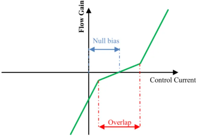
Among the different measures characterizing a servovalve, the flow gain curve is one of the most significative because it displays both static and dynamic features as shown in Fig. 3.
The extraction of this curve requires that the servovalve is equipped with flowmeters but in our application, only the position of the cylinder is measured. However, the cylinder’s velocity 𝑉𝑐𝑦𝑙and the servovalve output flows in each control
port 𝑄𝑆𝑉_ℎ𝑒𝑎𝑑 and 𝑄𝑆𝑉_𝑟𝑜𝑑 can be linked via the simplified
equation:
𝑉𝑐𝑦𝑙= {(𝑄𝑆𝑉_ℎ𝑒𝑎𝑑− 𝑄𝑐𝑜𝑜𝑙𝑖𝑛𝑔) 𝑆⁄ℎ𝑒𝑎𝑑 during shaft outlet −(𝑄𝑆𝑉_𝑟𝑜𝑑− 𝑄𝑐𝑜𝑜𝑙𝑖𝑛𝑔) 𝑆⁄ 𝑟𝑜𝑑 during shaft inlet
(1)
Where 𝑄𝑐𝑜𝑜𝑙𝑖𝑛𝑔is the cooling flow between the two sides of
the cylinder and 𝑆ℎ𝑒𝑎𝑑and 𝑆𝑟𝑜𝑑are respectively the
cross-sectional area of the head and the rod sides. Overlap Null bias Fl ow Ga in
Controller Servovalve Cylinder
LVDT Sensor
Fig. 1 : Schematic of the hydromechanical actuation loop
Torque Motor Flapper Spring
Spool
Control Current
B. Velocity Gain of a hydromechanical loop
In order to get around the lack of flowmeters to monitor the servovalve only, the idea is to monitor the whole loop by following salient features on the Velocity Gain curve.
This curve can be obtained only with the measures of both the control current 𝐼𝑐𝑜𝑛𝑡𝑟𝑜𝑙and the cylinder’s velocity 𝑉𝑐𝑦𝑙. The
value of 𝑉𝑐𝑦𝑙is computed by derivation of the cylinder’s
position 𝑋𝑐𝑦𝑙.
Blue points in Fig. 4 are the result of an extraction of the velocity gain curve performed during an entire flight. Because of the hysteresis of the servovalve, the dispersion of the points is substantial and therefore a smoothing algorithm based on local means is applied to the data.
The curve smoothing is performed on-board through a real-time algorithm in order to store the least possible data in the controller during the flight. Then the on-ground part consists in processing the information contained in the curve and carrying out the health monitoring procedure.
Fig. 4 : In-Flight extracted curve before and after smoothing
C. Indicators Construction
From the extracted curve, we define many indicators related to the targeted degradation. Those indicators are listed in Table I and their graphical equivalent is shown in Fig. 5.
TABLEI
INDICATORS EXTRACTED FROM THE CURVE
Names Targeted degradations Long Short
Slope change #1
abscissa 𝑋1 Degradations impacting the horizontal position of the curve Increase of the radial clearance between spool and sleeve Slope change #1
ordinate 𝑌1 Degradations impacting the vertical position of the curve Diaphragm clogging, cylinder internal leakage
Slope change #2
abscissa 𝑋2 Idem 𝑋1 Slope change #2
ordinate 𝑌2 Idem 𝑌1 Null Bias Current
𝐼𝑛𝑏=
𝑋1+ 𝑋2
2
𝐼𝑛𝑏 Degradations impacting the value of the
Null Bias
Null Bias current shift Idle Current of the
Loop (Current for null velocity)
𝐼0 Degradations impacting the static
behaviour of the loop All the degradations
Standard Deviation (hysteresis) at idle current
𝐻𝑦𝑠0 Degradations impacting the hysteresis
Increased Backlash Velocity Gain for
Shaft Inlet 𝐺𝑖𝑛 Degradations impacting the global dynamic behaviour of the loop Increased Backlash, Contamination of the filters, Increased friction force Velocity Gain for
Shaft Outlet 𝐺𝑜𝑢𝑡 Idem 𝐺𝑖𝑛 Velocity Gain for
Null Region 𝐺𝑛𝑢𝑙𝑙 Idem 𝐺𝑖𝑛
Fig. 5 : Graphical representation of the indicators
IV. DEGRADATIONS MODELING
A. Model and Sub-models Construction
A physical model of the hydromechanical system has been developed in Matlab-Simulink® in order to simulate its behaviour in presence of some degradation and to quantify their impacts. This model is composed of three sub-models: Servovalve, cylinder and controller. The granularity of the sub-models must be important enough to simulate all the degradations discussed in the system analysis. For example, the sub-model of the servovalve, the most complex one, must include the modelling of the two-stages, the filters and the feedback spring. A good method for modelling servovalves is given in [13].
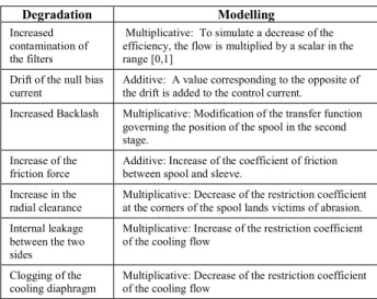
There are two ways degradations can be modelled: additive and multiplicative. The former consists in adding a value to some variables and the latter consists in a multiplication of some variables as shown in Erreur ! Source du renvoi introuvable.. In Erreur ! Source du renvoi introuvable., 𝑌𝑢 and 𝑈 are healthy values of
variables, 𝑓 is the degradation intensity and 𝑌 is the degraded value of variables.
8 10 12 14 16 18 20 22 -100 -80 -60 -40 -20 0 20 40 60 80 100
Control Current (mA)
C yl in d e r's V e lo ci ty (m m /s)
Raw Velocity Gain Curve Smoothed Curve
Cylinder’s Velocity (mm/s)
Control current (mA)
Shaft outlet velocity gain Shaft inlet velocity gain Null Region velocity gain Slope change #2 Slope change #1 Null Bias Current Idle Current of the Loop
Control current (mA)
Y = (A + f) U
ΣY
uY = Y
u+ f
f
U
f = Δa
aTABLEII MODELLINGOFDEGRADATIONS Degradation Modelling Increased contamination of the filters
Multiplicative: To simulate a decrease of the efficiency, the flow is multiplied by a scalar in the range [0,1]
Drift of the null bias
current Additive: A value corresponding to the opposite of the drift is added to the control current. Increased Backlash Multiplicative: Modification of the transfer function governing the position of the spool in the second stage.
Increase of the
friction force Additive: Increase of the coefficient of friction between spool and sleeve. Increase in the
radial clearance Multiplicative: Decrease of the restriction coefficient at the corners of the spool lands victims of abrasion. Internal leakage
between the two sides
Multiplicative: Increase of the restriction coefficient of the cooling flow
Clogging of the
cooling diaphragm Multiplicative: Decrease of the restriction coefficient of the cooling flow
B. Model Updating
The main hypothesis of this method is that operational data are available. Thus, it is supposed that the distribution of the indicators corresponding to a healthy state is well known.
For each simulation, the goal is to compute the velocity gain of the system by simulating the velocity of the cylinder for a gradually increasing control current from lower saturation boundary to upper saturation boundary.
Before simulating the degraded states, it is necessary to simulate and update the model parameters against operational data for the reference healthy state. Fig. 7 shows both extracted and estimated velocity gain curves for the healthy state. The estimated one is obtained from a model configured with averaged parameters given by constructors.
The result after model updating on parameters is also given in Fig. 7, and it can be noted that a difference remains between the curves around the idle current of the loop. The model used in this application is not enough accurate to explain this local deviation.
Fig. 7 : Extracted against Estimated Velocity Gain of the healthy state
C. Simulation of the degradations
For this paper, the focus will be on only two degradations namely the drift of the null bias current of the servovalve and the internal leakage between the two sides of the cylinder.
Results of the simulation on the updated model with those two degradations are given in Fig. 8.
Fig. 8 : (a) Left: effect of a null bias drift. (b) Right: effect of an internal leakage in the cylinder
V. INDICATORS TRANSFORMATION LAW COMPUTATION
A. Construction of the laws
In this part, a design of experiment is generated to organize the simulations of the behaviour of the system in presence of degradations. For each case, simulations are run for gradually increasing intensities of degradation. Eventually, the results are summarized in the form of indicators transformation laws (ITL).
With 𝐼𝑛𝑑𝑖 representing the 𝑖𝑡ℎ indicator in a healthy state,
𝐼𝑛𝑑𝑖𝑑𝑒𝑔 the 𝑖𝑡ℎ indicator in presence of the degradation 𝑑𝑒𝑔,
and 𝐼𝑛𝑡𝑑𝑒𝑔 the intensity of the degradation 𝑑𝑒𝑔, the ITL named 𝐹𝑖𝑑𝑒𝑔 corresponding to the 𝑖𝑡ℎ indicator and the
degradation 𝑑𝑒𝑔 can be defined as follows:
𝐼𝑛𝑡𝑑𝑒𝑔𝐹𝑖𝑑𝑒𝑔
→ ∆𝐼𝑖𝑑𝑒𝑔= 𝐴𝑖𝑑𝑒𝑔× 𝐼𝑛𝑡𝑑𝑒𝑔 (2)
Where𝐴𝑖𝑑𝑒𝑔is the coefficient of the linear regression of
∆𝐼𝑖𝑑𝑒𝑔with respect to 𝐼𝑛𝑡𝑑𝑒𝑔.∆𝐼
𝑖𝑑𝑒𝑔 is the change in the value of
the indicator and can be also expressed this way:
∆𝐼𝑖𝑑𝑒𝑔= 𝐼𝑛𝑑𝑖𝑑𝑒𝑔− 𝐼𝑛𝑑𝑖 (3)
Thus, 𝐹𝑖𝑑𝑒𝑔 provides the change in the indicator’s value for a given intensity of degradation.
B. Utilization of the laws
Once computed, an ITL makes it possible to generate an estimated value of indicators for a degraded state from a healthy value computed from operational data according to the following equation:
𝐼𝑖𝑑𝑒𝑔= 𝐼
𝑖ℎ𝑒𝑎𝑙𝑡ℎ𝑦+ ∆𝐼𝑖𝑑𝑒𝑔 (4)
In this application, 7 degradations and 10 indicators are considered, which means that 70 ITL must be computed. For instance, the law giving the value of 𝑋1for the degradation
drift of the null bias current is:
𝐼𝑋1𝑁𝐵 𝑑𝑟𝑖𝑓𝑡= 𝐼 𝑋1ℎ𝑒𝑎𝑙𝑡ℎ𝑦+ 𝐴𝑋1𝑁𝐵 𝑑𝑟𝑖𝑓𝑡× 𝐼𝑛𝑡𝑁𝐵 𝑑𝑟𝑖𝑓𝑡 (5) 10 12 14 16 18 20 22 -15 -10 -5 0 5 10 15
Control Current (mA)
C ylinde r's Velo cit y (m m /s )
Extracted Velocity Gain Curve from Datas Simulated Velocity Gain Curve before Recalibration Simulated Velocity Gain Curve after Recalibration
10 15 20 25 -20 -15 -10 -5 0 5 10 15 20
Control Current (mA)
C yli nd er 's V elo city (m m /s)
Simulated Velocity Gain Curve for Healthy State Simulated Velocity Gain Curve for a Drift of the Null Bias
11 12 13 14 15 16 17 18 19 20 -8 -6 -4 -2 0 2 4 6 8 10
Control Current (mA)
C yli nd er 's V elo city (m m /s)
Simulated Velocity Gain Curve for Healthy State Simulated Velocity Gain Curve for an Internal Leakage
Where 𝐼𝑋1ℎ𝑒𝑎𝑙𝑡ℎ𝑦is computed by averaging the extracted
value of X1 for a given number of flights for which the
system is considered flawless.
VI. STATISTICAL VALIDATION OF PERFORMANCES
A. Key Performance Indicators
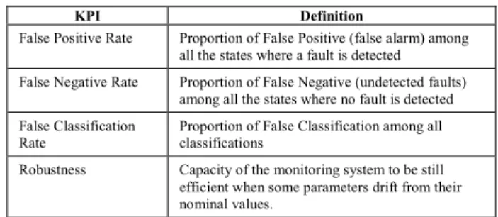
For this application, both fault detection and diagnosis are addressed. A presentation and definition of Key Performance Indicators (KPI) is given in Table III.
TABLEIII
KEYPERFORMANCEINDICATORS
KPI Definition
False Positive Rate Proportion of False Positive (false alarm) among all the states where a fault is detected False Negative Rate Proportion of False Negative (undetected faults)
among all the states where no fault is detected False Classification
Rate Proportion of False Classification among all classifications Robustness Capacity of the monitoring system to be still
efficient when some parameters drift from their nominal values.
B. Method for fault detection and diagnosis
A more precise presentation of the method presented below can be found in [14].
1) Indicators Model Learning:
The first step is to learn a Gaussian model of the indicators distribution in a reference state, typically a healthy state. The model is learned from extracted indicators on a given number of flights and is presented as follows:
𝑀𝑜𝑑𝑒𝑙(𝑖) = (𝜇𝑖
ℎ𝑒𝑎𝑙𝑡ℎ𝑦
𝜎𝑖ℎ𝑒𝑎𝑙𝑡ℎ𝑦) (6)
Where 𝜇𝑖ℎ𝑒𝑎𝑙𝑡ℎ𝑦 is the mean of the indicators and
𝜎𝑖ℎ𝑒𝑎𝑙𝑡ℎ𝑦their standard deviation. 2) Fault Detection:
It is based on an abnormality score named 𝑍𝑠𝑐𝑜𝑟𝑒. For the indicator 𝑖, 𝑍𝑠𝑐𝑜𝑟𝑒,𝑖is defined as follows:
𝑍𝑠𝑐𝑜𝑟𝑒,𝑖=𝐼𝑖− 𝜇𝑖ℎ𝑒𝑎𝑙𝑡ℎ𝑦
𝜎𝑖ℎ𝑒𝑎𝑙𝑡ℎ𝑦 (7)
Where 𝐼𝑖is the currently measured value of indicator.
Then a global abnormality score of the system 𝐺𝑙𝑜𝑏𝑎𝑙_𝑍𝑠𝑐𝑜𝑟𝑒 is computed from 𝑍𝑠𝑐𝑜𝑟𝑒,𝑖with 𝑖 ∈
[1; 10] via the Mahalanobis distance [15].
Indicators are extracted on-board and 𝐺𝑙𝑜𝑏𝑎𝑙_𝑍𝑠𝑐𝑜𝑟𝑒is computed on-ground at each flight. The parameterization of the fault detection consists in defining a relevant threshold value 𝑇ℎ𝑟 and if the value of 𝐺𝑙𝑜𝑏𝑎𝑙_𝑍𝑠𝑐𝑜𝑟𝑒crosses 𝑇ℎ𝑟, it means that a fault has been detected.
3) Diagnosis:
Diagnosis is performed via a classification of signatures. A signature is a vector of indicators. For this application, a
signature is a vector appending 10 indicators extracted from flight data:
𝑆𝑖𝑔𝑛 = (𝑍𝑠𝑐𝑜𝑟𝑒,𝑋1, 𝑍𝑠𝑐𝑜𝑟𝑒,𝑌1, … , 𝑍𝑠𝑐𝑜𝑟𝑒,𝐺𝑛𝑢𝑙𝑙)
𝑇
(8) If the system is healthy, 𝑆𝑖𝑔𝑛 is a zero vector of size 10. Assuming that the maximal intensities of the degradations are known, it is possible to determine the signatures of the degradations 𝑆𝑖𝑔𝑛𝑟𝑒𝑓,𝑑𝑒𝑔 associated. 𝑆𝑖𝑔𝑛𝑟𝑒𝑓,𝑑𝑒𝑔= (𝐼𝑋1 𝑑𝑒𝑔− 𝜇 𝑋1 ℎ𝑒𝑎𝑙𝑡ℎ𝑦 𝜎𝑋ℎ𝑒𝑎𝑙𝑡ℎ𝑦1 , … , 𝐼𝐺𝑑𝑒𝑔𝑛𝑢𝑙𝑙− 𝜇 𝐺𝑛𝑢𝑙𝑙 ℎ𝑒𝑎𝑙𝑡ℎ𝑦 𝜎𝐺ℎ𝑒𝑎𝑙𝑡ℎ𝑦𝑛𝑢𝑙𝑙 ) 𝑇 (9) When a fault is detected, the classification algorithm is run. This algorithm is based on a pattern recognition method which finds the reference signature that most closely matches the currently measured signature. A guilt probability is assigned to each component of the system. C. Statistical Validation
1) Matrix of the signatures
To perform fault detection and diagnosis, it is essential to determine the matrix of the signatures. It shows the signature corresponding to the maximal intensity of the degradations. A part of this matrix, taking into account only two degradations is given in Table IV.
TABLEIV
MATRIXOFTHESIGNATURES
Degradatio
n 𝑋 Influences (𝒁𝒔𝒄𝒐𝒓𝒆𝒔)
1 𝑌1 𝑋2 𝑌2 𝐼𝑛𝑏 𝐼0 𝐻𝑦𝑠0 𝐺𝑖𝑛 𝐺𝑜𝑢𝑡 𝐺𝑛𝑢𝑙𝑙
Drift of the null
bias current 24 0 26 0 28 24 0 0 0 0 Internal leakage
between the two
sides 0 4 0 11 0 1 0 0 0 0
2) Performances of fault detection
Once the matrix of the signatures is available, a detection threshold 𝑇ℎ𝑟 on the global score 𝐺𝑙𝑜𝑏𝑎𝑙_𝑍𝑠𝑐𝑜𝑟𝑒must be defined.
The value of this threshold must be low enough to ensure detection of all the different degradation, even those not provided by the system analysis and high enough to ensure a low rate of false alarms. To set this value in an optimal way, it is essential to take into account the standard deviation of the 𝐺𝑙𝑜𝑏𝑎𝑙_𝑍𝑠𝑐𝑜𝑟𝑒.
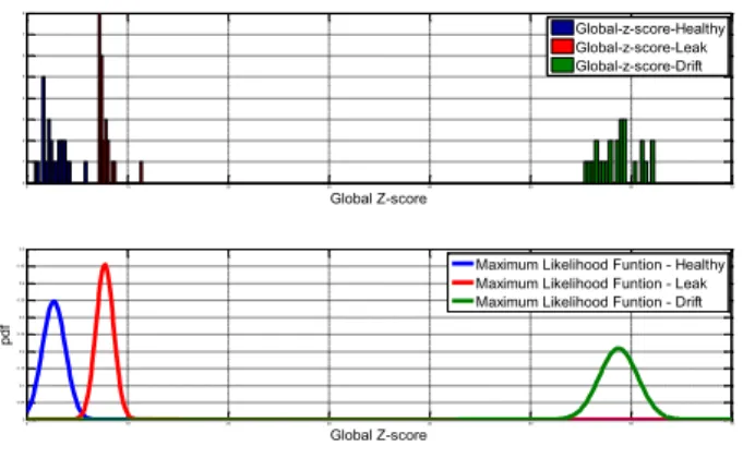
First, the computation of the probability density function of 𝐺𝑙𝑜𝑏𝑎𝑙_𝑍𝑠𝑐𝑜𝑟𝑒−ℎ𝑒𝑎𝑙𝑡ℎ𝑦is performed to set a first value of 𝑇ℎ𝑟, as shown in Fig. 9. Typically, the chosen value for 𝑇ℎ𝑟 is:
𝑇ℎ𝑟 = 𝜇ℎ𝑒𝑎𝑙𝑡ℎ𝑦+ 𝐴 × 𝜎ℎ𝑒𝑎𝑙𝑡ℎ𝑦 (10)
At first approach, the chosen value for 𝐴 is 𝐴 = 2 because it ensures that only 5% of false detection. However, this value can potentially limit the false negative rate so it is necessary to check if the degradations are still detectable.
To ensure the performances, the distributions of 𝐺𝑙𝑜𝑏𝑎𝑙_𝑍𝑠𝑐𝑜𝑟𝑒−ℎ𝑒𝑎𝑙𝑡ℎ𝑦,𝐺𝑙𝑜𝑏𝑎𝑙_𝑍𝑠𝑐𝑜𝑟𝑒−𝑙𝑒𝑎𝑘 and 𝐺𝑙𝑜𝑏𝑎𝑙_𝑍𝑠𝑐𝑜𝑟𝑒−𝑑𝑟𝑖𝑓𝑡 are compared as presented in Fig. 9.
Performances for different values of 𝐴 are presented in Table V.
Fig. 9 : Distribution of Global_scores and likelihood functions TABLEV
FAULTDETECTIONPERFORMANCES
𝐴
Null Bias Drift Internal Leakage False
Positive False Negative False Positive False Negative
0 0% 0% 50% 0%
1 0% 0% 16% 0%
2 0% 0% 3% 0%
3 0% 0% 0.3% 2%
3) Performances of diagnosis
The classification algorithm gives, for each component of the system, a probability of guilt proportional to the colinearity between the current signature and the referenced signatures. The diagnosis performances depend on the intensity of the degradations. Results are shown in Table VI.
TABLEVI
DIAGNOSISPERFORMANCES
Effective
Degradation Percentage of max intensity (From ITL) Probability of guilt of Drift Probability of guilt of Leak
Drift 25% 0.94 0.06 Drift 50% 0.94 0.06 Drift 100% 0.94 0.06 Leak 25% 0.37 0.63 Leak 50% 0.13 0.87 Leak 100% 0.11 0.89 VII. CONCLUSION
This paper provides a methodology to perform fault detection and diagnosis on a hydromechanical actuation loop. A first part details how to construct relevant indicators to perform on-board extraction of indicators and a second part how to achieve and validate fault detection and diagnosis on-ground. It must be noted that further works will follow, dealing with the management of uncertainties, the architecture of monitoring for a wider system and also prognostics.
REFERENCES
[1] J. Sheppard, M. Kaufman et T. Wilmer, «IEEE Standards for Prognostics and Health Management,» Aerospace and
Electronic Systems Magazine, vol. 24, n° %19, p. 34–41,
2009.
[2] A. Jardine, D. Lin et D. Banjevic, «A review on machinery diagnosis and prognostics implementing condition-based maintenance,» Mechanical systems and signal processing, vol. 20, n° %17, p. 1483–1510, 2006.
[3] B. Saha et K. Goebel, «Uncertainty management for diagnosis and prognostics of batteries using Bayesian techniques,» chez
IEEE Aerospace Conference, Big Sky, 2008.
[4] A. Muller, Contribution à la maintenance prévisionnelle des systèmes de production par la formalisation d'un processus de pronostic, PhD thesis from the Nancy I University - Henri Poincaré, 2005.
[5] P. Ribot, Vers l'intégration diagnostic-pronostic pour la maintenance des systèmes complexes, PhD thesis from the Toulouse III University - Paul Sabatier, 2009.
[6] P. Cocheteux, Contribution à la maintenance proactive par la formalisation du processus de pronostic des performances de systèmes industriels, PhD thesis from the Nancy I University - Henri Poincaré, 2010.
[7] J. Massé, B. Lamoureux and X. Boulet, "Prognosis and Health Management in system design," in IEEE International
Conference on Prognostics and Health Management, Denver,
2011.
[8] A. Patterson-Hine, G. Biswas, G. Aaseng, S. Narasimhan et K. Pattipati, «A Review of Diagnostic Techniques for ISHM Applications,» vol. 1st Integrated Systems Health Engineering and Management Forum, 2005.
[9] M. Roemer, C. S. Byington, G. Kacprzynski et G. Vachtsevanos, «An overview of selected prognostic technologies with application to engine health management,» chez Proceedings of GT2006 ASME Turbo Expo , Barcelona, 2006.
[10] N. Mechbal, M. Vergé, G. Coffignal and M. Ganapathi, "Application of a combined active control and fault detection scheme to an active composite flexible structure,"
Mechatronics vol. 16, pp. 193-208, 2006.
[11] L. Borello, M. D. Vedova, G. Jacazio et M. Sorli, «A Prognostic Model for Electrohydraulic Servovalves,» Annual
Conference of the Prognostics and Health Management Society, 2009.
[12] P.-Y. Crepin et R. Kress, «Model Based Fault Detection for an Aircraft Actuator,» chez 22nd Congress of International
Council of the Aeronautical Sciences, Harrogate, 2000.
[13] B. Attar, Modélisation réaliste en conditions extrêmes des servovalves électrohydrauliques utilisées pour le guidage et la navigation aéronautique et spatiale, Thèse de l’Université de Toulouse, délivré par l’INSA de Toulouse, 2008.
[14] J. Lacaille, «Standardized failure signature for a turbofan engine,» chez Aerospace conference, 2009 IEEE , Big Sky, MT, 2009.
[15] R. De Maesschalck, D. Jouan-Rimbaud et D. Massart, «The mahalanobis distance,» Chemometrics and Intelligent
Laboratory Systems, vol. 50, n° %11, pp. 1-18, 2000.
0 10 20 30 40 50 60 70 0 1 2 3 4 5 6 7 8 Global Z-score 0 10 20 30 40 50 60 70 0 0.05 0.1 0.15 0.2 0.25 0.3 0.35 0.4 0.45 0.5 Global Z-score pdf
Maximum Likelihood Funtion - Healthy Maximum Likelihood Funtion - Leak Maximum Likelihood Funtion - Drift Global-z-score-Healthy Global-z-score-Leak Global-z-score-Drift