HAL Id: tel-01400198
https://pastel.archives-ouvertes.fr/tel-01400198
Submitted on 21 Nov 2016HAL is a multi-disciplinary open access archive for the deposit and dissemination of sci-entific research documents, whether they are pub-lished or not. The documents may come from teaching and research institutions in France or
L’archive ouverte pluridisciplinaire HAL, est destinée au dépôt et à la diffusion de documents scientifiques de niveau recherche, publiés ou non, émanant des établissements d’enseignement et de recherche français ou étrangers, des laboratoires
Pauline Sarrabezolles
To cite this version:
Pauline Sarrabezolles. Colourful linear programming. General Mathematics [math.GM]. Université Paris-Est, 2015. English. �NNT : 2015PESC1033�. �tel-01400198�
Ecole Doctorale M
ATHÉMATIQUES ETS
CIENCES ETT
ECHNOLOGIES DE L’I
NFORMATION ET DE LAC
OMMUNICATIONT
HÈSE DE DOCTORAT
Spécialité : Mathématiques appliquées
Présentée par
Pauline S
ARRABEZOLLES
Pour obtenir le grade de
D
OCTEURde l’U
NIVERSITÉP
ARIS-E
STC
OLORFUL LINEAR PROGRAMMING
Soutenance prévue le 6 juillet 2015 devant le jury composé de :
Victor C
HEPOI Aix-Marseille Université RapporteurJesus D
EL
OERA University of California RapporteurAntoine D
EZA Hamilton University ExaminateurXavier G
OAOC Université Paris-Est ExaminateurNabil M
USTAPHA Université Paris-Est ExaminateurAndrás S
EBÖ Université de Grenoble ExaminateurWolfgang M
ÜLZER Freie Universität Berlin InvitéIf you want to make peace with your enemy, you have to work with your enemy. Then he becomes your partner. —Nelson Mandela
Remerciements
Je tiens à remercier en premier lieu mon directeur de thèse, Frédéric Meunier. Attentif et disponible, c’est un directeur hors pair, un soutien précieux et constant et une source inépuisable d’idées et de pistes de recherche. Je souhaite lui témoigner ma gratitude pour ses nombreux conseils et ses méticuleuses relectures, mais aussi et surtout pour le temps passé à “faire de la recherche”, c’était un vrai plaisir.
J’adresse mes sincères remerciements à Jesus De Loera et à Victor Chepoi pour avoir accepté d’être rapporteurs de cette thèse. Merci également aux examinateurs qui ont accepté de siéger dans le jury de ma soutenance.
Je souhaite également remercier tous les chercheurs avec qui j’ai collaboré. J’ai une pensée chaleureuse pour Max Klimm et Yann Disser, ainsi que pour Wolfgang Mülzer et Yannik Stein. Je remercie bien sûr tout particulièrement Antoine Deza qui m’a acceuillie à Hamilton et a fait naitre chez moi la fièvre de la programmation linéaire colorée. Enfin je remercie Shmuel Onn, pour son hospitalité et pour nos longues dis-cussions sur les chemins du mont Carmel, qui bien qu’interrompues trop tôt restent parmi mes meilleurs souvenirs dans la recherche.
Je souhaite évidemment remercier le Cermics, qui m’a offert les meilleurs con-ditions de travail que peut espérer un doctorant. Je remercie l’université Paris-Est et en particulier Sylvie Cach, pour sa grande disponibilité et sa bonne humeur com-municative. J’adresse enfin mes remerciements à l’équipe du Programme Gaspard Monge pour la recherche Opérationnelle et l’Optimisation, et en particulier à Sandrine Charousset.
Vient le tour des amis et de la famille, auxquels j’ajouterais ma marraine la bonne fée Isabelle, perle du Cermics. Merci à vous tous, d’avoir veiller sur moi. Un merci par-ticulier à Mamy, pour son soutien depuis toujours, dans les moments joyeux comme dans les moments difficiles. Merci à Alex, Charly et Camou, à mes collocs Soupa et Maria, au BB, à Paraj et Nina, aux Wild Boars et bien sûr à Emmanuel. Merci à tous
les doctorants : les joueurs de tennis (William et Xavier), les coureurs (Axel, Yannick, Laurents et François), les preneurs de café et autres boissons protéïnées (Houssam, Nahia et Pierre), les gentils organisateurs du séminaire (David et Clément), les anciens (Oussam, Daniel, Thomas, Rafik, Adela, ...) merci pour les bons moments passés en-semble, et meilleurs voeux à ceux dont c’est bientôt le tour.
Enfin, je tiens à remercier Manou, à qui je dédie ce manuscrit. Merci pour tous ces bons moments au coin du feu, où nous nous amusions à faire des maths. En m’apprenant à jouer à la géométrie, tu m’as fait un cadeau immense qui m’a conduite jusqu’ici.
Abstract
The colorful Carathéodory theorem, proved by Bárány in 1982, states the following. Given d + 1 sets of points S1, . . . , Sd +1⊆ Rd, each of them containing 0 in its convex
hull, there exists a colorful set T containing 0 in its convex hull, i.e. a set T ⊆Sd +1
i =1Si
such that |T ∩ Si| ≤ 1 for all i and such that 0 ∈ conv(T ). This result gave birth to
several questions, some algorithmic and some more combinatorial. This thesis provides answers on both aspects.
The algorithmic questions raised by the colorful Carathéodory theorem concern, among other things, the complexity of finding a colorful set under the condition of the theorem, and more generally of deciding whether there exists such a colorful set when the condition is not satisfied. In 1997, Bárány and Onn defined colorful linear programming as algorithmic questions related to the colorful Carathéodory theorem. The two questions we just mentioned come under colorful linear programming. This thesis aims at determining which are the polynomial cases of colorful linear program-ming and which are the harder ones. New complexity results are obtained, refining the sets of undetermined cases. In particular, we discuss some combinatorial versions of the colorful Carathéodory theorem from an algorithmic point of view. Furthermore, we show that computing a Nash equilibrium in a bimatrix game is polynomially re-ducible to a colorful linear programming problem. On our track, we found a new way to prove that a complementarity problem belongs to the PPAD class with the help of Sperner’s lemma. Finally, we present a variant of the “Bárány-Onn” algorithm, which is an algorithm computing a colorful set T containing 0 in its convex hull whose exis-tence is ensured by the colorful Carathéodory theorem. Our algorithm makes a clear connection with the simplex algorithm. After a slight modification, it also coincides with the Lemke method, which computes a Nash equilibrium in a bimatrix game. The combinatorial question raised by the colorful Carathéodory theorem concerns the number of positively dependent colorful sets. Deza, Huang, Stephen, and Terlaky (Colourful simplicial depth, Discrete Comput. Geom., 35, 597–604 (2006)) conjectured that, when |Si| = d + 1 for all i ∈ {1, . . . , d + 1}, there are always at least d2+ 1 colourful
sets containing 0 in their convex hulls. We prove this conjecture with the help of combinatorial objects, known as the octahedral systems. Moreover, we provide a
Résumé
Le théorème de Carathéodory coloré, prouvé en 1982 par Bárány, énonce le résultat suivant. Etant donnés d + 1 ensembles de points S1, . . . , Sd +1dansRd, si chaque Si
contient 0 dans son enveloppe convexe, alors il existe un sous-ensemble arc-en-ciel T ⊆Sd +1
i =1Si contenant 0 dans son enveloppe convexe, i.e. un sous-ensemble T tel que
|T ∩ Si| ≤ 1 pour tout i et tel que 0 ∈ conv(T ). Ce théorème a donné naissance à de
nombreuses questions, certaines algorithmiques et d’autres plus combinatoires. Dans ce manuscrit, nous nous intéressons à ces deux aspects.
En 1997, Bárány et Onn ont défini la programmation linéaire colorée comme l’ensemble des questions algorithmiques liées au théorème de Carathéodory coloré. Parmi ces questions, deux ont particulièrement retenu notre attention. La première concerne la complexité du calcul d’un sous-ensemble arc-en-ciel comme dans l’énoncé du théorème. La seconde, en un sens plus générale, concerne la complexité du problème de décision suivant. Etant donnés des ensembles de points dansRd, correspondant aux couleurs, il s’agit de décider s’il existe un sous-ensemble arc-en-ciel contenant 0 dans son enveloppe convexe, et ce en dehors des conditions du théorème de Carathéodory coloré. L’objectif de cette thèse est de mieux délimiter les cas polynomiaux et les cas “difficiles” de la programmation linéaire colorée. Nous présentons de nouveaux
résul-tats de complexités permettant effectivement de réduire l’ensemble des cas encore incertains. En particulier, des versions combinatoires du théorème de Carathéodory coloré sont présentées d’un point de vue algorithmique. D’autre part, nous montrons que le problème de calcul d’un équilibre de Nash dans un jeu bimatriciel peut être réduit polynomialement à la programmation linéaire coloré. En prouvant ce dernier résultat, nous montrons aussi comment l’appartenance des problèmes de complé-mentarité à la classe PPAD peut être obtenue à l’aide du lemme de Sperner. Enfin, nous proposons une variante de l’algorithme de Bárány et Onn, calculant un sous-ensemble arc-en-ciel contenant 0 dans son enveloppe convexe sous les conditions du théorème de Carathéodory coloré. Notre algorithme est clairement relié à l’algorithme du simplexe. Après une légère modification, il coïncide également avec l’algorithme de Lemke, calculant un équilibre de Nash dans un jeu bimatriciel.
le nombre de sous-ensemble arc-en-ciel contenant 0 dans leurs enveloppes con-vexes. Deza, Huang, Stephen et Terlaky (Colourful simplicial depth, Discrete Comput. Geom., 35, 597–604 (2006)) ont formulé la conjecture suivante. Si |Si| = d + 1 pour
tout i ∈ {1,...,d + 1}, alors il y a au moins d2+ 1 sous-ensemble arc-en-ciel contenant 0 dans leurs enveloppes convexes. Nous prouvons cette conjecture à l’aide d’objets combinatoires, connus sous le nom de systèmes octaédriques, dont nous présentons une étude plus approfondie.
Contents
Acknowledgements 1
Abstract (English/Français) 3
List of figures 11
Introduction 13
1 The colorful Carathéodory theorem and its relatives 21
1.1 Definitions and preliminaries . . . 21
1.1.1 Basic geometric notions . . . 21
1.1.2 Linear programming . . . 22
1.1.3 General position, degeneracy, perturbation . . . 23
1.1.4 Polytope, polyhedron, triangulation . . . 24
1.2 The Colorful Carathéodory theorem: various formulations . . . 25
1.3 Proofs of the colorful Carathéodory theorem . . . 26
1.3.1 Original proof by Bárány . . . 26
1.3.2 Sperner’s lemma proves the colorful Carathéodory theorem . . . . 28
1.4 Applications in geometry . . . 30
1.4.1 Tverberg’s theorem . . . 30
1.4.2 First selection lemma . . . 31
1.4.3 Weakε-nets . . . 32
1.5 Octahedron lemma: three proofs . . . 32
1.5.1 Topological proof . . . 33
1.5.2 Parity proof argument . . . 33
1.5.3 Geometric proof . . . 35
1.6 Other colorful results in geometry . . . 36
1.6.1 Colored Tverberg’s theorem . . . 36
2 Computational problems 39
2.1 Colorful linear programming, TFNP version . . . 39
2.1.1 Definition . . . 39
2.1.2 Simplexification of Bárány-Onn algorithm . . . 40
2.2 Colorful linear programming, decision version . . . 44
2.3 Find another colorful simplex . . . 46
2.3.1 Main result . . . 46
2.3.2 FIND ANOTHERis PPAD-complete . . . 47
2.3.3 Reduction of BIMATRIXto COLORFULLINEARPROGRAMMING . . . 50
2.4 Combinatorial cases of colorful linear programming and analogues . . . 51
2.4.1 Colorful linear programming, TFNP version . . . 51
2.4.2 Colorful linear programming, decision version . . . 53
2.4.3 Combinatorial cases of FIND ANOTHER . . . 55
2.4.4 Similar combinatorial problems . . . 57
3 A generalization of linear programming and linear complementarity 59 3.1 A generalization of linear programming . . . 59
3.1.1 Generalization of linear programs: feasibility, optimization . . . . 59
3.1.2 Polyhedral interpretations, almost colorful connectivity . . . 62
3.1.3 A generalization of colorful linear programming . . . 65
3.2 A generalization of linear complementarity . . . 71
3.2.1 The linear complementarity problem . . . 71
3.2.2 The Lemke method . . . 72
3.2.3 The Lemke-Howson algorithm for BIMATRIX . . . 74
4 Octahedral systems 77 4.1 Octahedral systems . . . 77 4.1.1 Definition . . . 77 4.1.2 Motivation . . . 78 4.1.3 First properties . . . 79 4.2 Decomposition . . . 80
4.3 Other properties of octahedral systems . . . 82
4.3.1 Geometric interpretation of the decomposition . . . 82
4.3.2 Further uses of umbrellas and discussions . . . 84
4.3.3 Realizability . . . 85
4.3.4 Number of octahedral systems . . . 88
5 Octahedral systems: computation of bounds 91 5.1 Upper bounds . . . 91
Contents
5.2.1 Preliminaries . . . 94
5.2.2 Proof of the main result . . . 95
5.2.3 Other bounds . . . 99
5.3 The colorful simplicial depth conjecture . . . 106
5.3.1 Proof of the original conjecture . . . 106
5.3.2 A more general conjecture . . . 107
Bibliography 113
List of Figures
1 The Carathéodory theorem in dimension 2 . . . 13
2 The colorful Carathéodory theorem in dimension 2 . . . 14
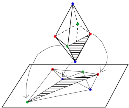
3 A colorful point configuration inR3with 10 colorful tetrahedra contain-ing p . . . 17
1.1 Bárány’s proof of the colorful Carathéodory theorem . . . 27
1.2 A Sperner labeling in dimension 2 . . . 28
1.3 The Octahedron lemma in dimension 2 . . . 33
1.4 Affine mapping of the crosspolytope . . . 34
2.1 Construction of D for the formula (x1∨x2∨ ¯x3)∧(x1∨ ¯x2∨x3)∧( ¯x1∨ ¯x2∨x3) 54 3.1 Reduction of a bounded conic case to a convex case . . . 63
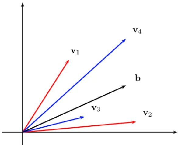
3.2 Colorful configuration definingP = ©x ∈ R4|P xivi= b, x ≥ 0 ª . . . 63
3.3 PolyhedronP = ©x ∈ R4|P xivi= b, x ≥ 0ª defined in Figure 3.2 . . . 64
4.1 An umbrella of color V3 . . . 80
4.2 The complete octahedral system . . . 84
4.3 A non realizable (3, 3, 3)-octahedral system with 9 edges . . . 86
4.4 Decomposition of the (3, 3, 3)-octahedral system of Figure 4.3 . . . 86
4.5 Proof of the non realizability of the (3, 3, 3)-octahedral system of Figure 4.3 87 5.1 Construction ofΩ(4,2)⊆ V1× · · · × V7with |V1| = · · · = |V7| = 4 . . . 92
5.2 Ω(4,2)⊆ V1× · · · × V7with |Vi| = 4 for all i . . . 93
5.3 The vertex set of the (m1, . . . , mn−k, k, . . . , k, k − 1,...,k − 1)-octahedral systemΩ ⊆ V1× · · · × Vnused for the proof of Proposition 5.2.14 . . . 104
Introduction
The colorful Carathéodory theorem
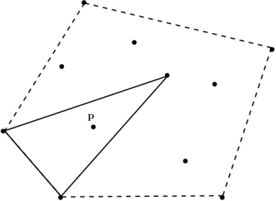
Given a set S of N ≥ 3 points in the plane and a point p in the convex hull of S, there is a triangle formed with points of S containing p in its convex hull. In general dimension d , the Carathéodory theorem states the following. Given a set S of N ≥ d + 1 points in Rd
and a point p in the convex hull of S, there is a subset T ⊆ S of size at most d + 1 containing p in its convex hull.
b b b b b b b b b b b p
Figure 1: The Carathéodory theorem in dimension 2
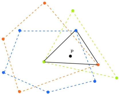
Bárány [2] proposed a generalization of this theorem, in which S is partitioned into d + 1 sets, or colors, and the set T is colorful, i.e. it intersects each color at most once. Consider blue points, green points, and red points in the plane, such that there is a point p simultaneously in the convex hull of the blue points, in the convex hull of
the green points, and in the convex hull of the red points. The colorful Carathéodory theorem, proved by Bárány in 1982, ensures the existence of a colorful triangle, i.e. a tri-angle formed with one blue point, one green point, and one red point, also containing p in its convex hull.
In general dimension d , the colorful Carathéodory theorem states the following.
Theorem. Given d + 1 sets S1, . . . , Sd +1, and any point p ∈Td +1i =1conv(Si), there is a
colorful set T containing p in its convex hull, that is a set T ⊆Sd +1
i =1Sisuch that |T ∩Si| ≤
1 for all i ∈ [d + 1], and p ∈ conv(T ).
b b b b b b b b b b b b b b p
Figure 2: The colorful Carathéodory theorem in dimension 2
The colorful Carathéodory theorem gave birth to this thesis and motivated most of the questions we considered during the course of my Doctoral study. Two main streams of questions are raised by this theorem: the computational problems on the one hand and a more combinatorial problem on the other hand. In the remaining of this introduction, we present these two streams. We end the introduction with applications of colorful linear programming.
Computational problems
A natural question raised by the colorful Carathéodory theorem is whether a colorful set containing p in its convex hull can be computed in polynomial time. The case
Introduction
with S1= · · · = Sd +1, corresponding to the usual Carathéodory theorem, is known to be
computable in polynomial time via linear programming. However, the complexity of the colorful version remains an open question.
A second problem concerns the complexity of deciding whether there exists such a colorful set, in case the conditions of the colorful Carathéodory are not satisfied. More precisely, given k sets S1, . . . , Sk inRd and a point p ∈ Rd, the problem is to decide
whether there is a colorful set containing p in its convex hull, i.e. a set T ⊆Sk
i =1Si
such that |T ∩ Si| ≤ 1 for all i ∈ [d + 1] and p ∈ conv(T ). This problem, often referred to
as the colorful linear programming problem, is known to be NP-complete in general. Depending on the context, we may consider this problem with a linear programming point of view. Formally, the problem is the following. Given a d × n matrix A ∈ Rd ×n, a vector b ∈ Rd, and a partition of [n] into k sets I1, . . . , Ik, decide whether there exists a
solution x ∈ Rnto the system
Ax = b,
x ≥ 0, (1)
| supp(x) ∩ Ij| ≤ 1, for all j ∈ [k],
where supp(x) is the set {i ∈ [n] | xi 6= 0}. We show that the problems of deciding
whether a colorful solution exists and of optimizing a linear cost function over all colorful solutions can be polynomially reduced one to the other. Colorful linear pro-gramming either refers to one or the other version. A seemingly more general problem is obtained by replacing the constraints on the support by |supp(x) ∩ Ij| ≤ `j for all
j ∈ [k], for some prefixed `j ∈ Z+. We discuss the complexity of this generalization
and get some partial results in Chapter 3. A polyhedral interpretation of colorful linear programming is also provided in the same chapter.
Another computational problem is raised by the Octahedron lemma, which is a the-orem similar to the colorful Carathéodory. This thethe-orem states that given d + 1 pairs of points inRd and a point p ∈ Rd, all in general position, there is an even number of colorful sets containing p in their convex hulls. In particular, it shows that if p is contained in the convex hull of a colorful set, then p is contained in the convex hull of another colorful set. The related computational problem, known as find another colorful simplex is the following. Given d + 1 pairs of points in Rd and a point p ∈ Rd, all in general position, and given a colorful set containing p in its convex hull, compute another colorful set containing p in its convex hull. The complexity of this problem was an open question.
provide combinatorial polynomial cases of the colorful Carathéodory theorem. We propose a variant of the “Bárány-Onn” algorithm, which computes a colorful set con-taining 0 in its convex hull. Our algorithm makes a clear connection with the simplex algorithm. We also extended the result of Bárány and Onn on the NP-completeness of colorful linear programming to the case with k = d + 1, answering one of their ques-tions. Finally we proved that find another colorful simplex is PPAD-complete. The most surprising result we obtain is the fact that colorful linear programming contains the problem of finding a Nash equilibrium in a bimatrix game. Most of these results, presented in Chapter 2, can be found in the article
F. Meunier and P. Sarrabezolles. Colorful linear programming, Nash equi-librium, and pivots. Discrete Applied Mathematics, under revision.
The colorful simplicial depth conjecture
Simplicial depth
Given a set S of real numbers, the median is a real number m such that half the numbers in S are not larger than m and half the numbers in S are not smaller than m. A median can equivalently be defined as a real number contained in the largest possible number of segments [a, b] with a, b ∈ S.
In 1990, Liu [35] generalized the concept of median in higher dimension. This general-ization, known as deepest point, is the following: given a set S of points inRd, a deepest point is a point m ∈ Rd contained in the largest possible number of simplices formed with points of S. This notion has many applications in statistics and in data analysis.
A natural question raised by this notion is how deep is a deepest point, i.e. what is the maximal number of simplices formed with points of S whose convex hulls intersect? This geometric question has been asked earlier, and a first answer was given by Bárány using the colorful Carathéodory theorem.
Colorful simplicial depth
Liu’s notion can be extended to the colorful point configurations. Given d + 1 sets S1, . . . , Sd +1of points inR and a point p ∈ Rd, we define the colorful simplicial depth
of p to be the number of colorful sets containing p in their convex hulls. The colorful Carathéodory theorem shows that under the conditions of the theorem, there is a point with colorful simplicial depth at least equal to 1. On Figure 2, a point p as in the
Introduction
statement and a colorful triangle containing it are represented. There are in fact more colorful triangles containing this point p.
In 2006, Deza et al. [17] conjectured that if each Si is of size at least d + 1, then any
point p ∈Td +1
i =1 conv(Si) is contained in the convex hulls of at least d
2+ 1 colorful sets.
They proved in the same paper that the bound d2+ 1 is tight. As a matter of fact, there are colorful point configurations, with d + 1 sets of d + 1 points in Rd, such that there is a point p ∈Td +1
i =1conv(Si) contained in the convex hulls of exactly d
2+ 1 colorful sets,
see Figure 3 for such a configuration in dimension 3.
b b b b b b b b bb b b b b b b b p
Figure 3: A colorful point configuration inR3with 10 colorful tetrahedra containing p
Bárány suggested a combinatorial approach to this problem. It consists in considering a special class of hypergraphs generalizing the colorful point configuration, the octahe-dral systems. Given a colorful point configuration, there is a corresponding octaheoctahe-dral system, whose edges are identified with the colorful sets containing 0 in their convex hulls. Hence a bound on the number of edges in an octahedral system gives a bound on the colorful simplicial depth. The octahedral systems are studied in Chapter 4 and Chapter 5. Using this approach, we improve the best known bound. This work appeared in the article
A. Deza, F. Meunier, and P. Sarrabezolles. A combinatorial approach to colourful simplicial depth. SIAM Journal on Discrete Mathematics, 28(1): 306–322, 2014.
Finally, we prove the colorful simplicial depth conjecture, using the same approach. This proof appeared in the article
P. Sarrabezolles. The colorful simplicial depth conjecture. Journal of Com-binatorial Theory, Series A, 130(0): 119–128, 2015.
Our proof actually shows that if each Si is of size m ≥ d + 1, then any point p ∈
Td +1
i =1 conv(Si) is contained in the convex hulls of at least (m − 2)(d + 1) + 2 colorful
sets.
More generally, we formulate the following conjecture.
Conjecture. Consider a colorful point configuration with |S1| ≥ · · · ≥ |Sd +1| ≥ d + 1 ≥ 2.
Any point p ∈Td +1
i =1 conv(Si) is contained in the convex hulls of at least d +1
X
i =1
(|Si| − 2) + 2
colorful sets.
Applications of colorful linear programming
The study of problems related to the colorful Carathéodory theorem is usually moti-vated in the literature by the many theoretical applications of this result in geometry, and by the challenging questions raised by these problems. We would like to give another motivation here, with practical applications of colorful linear programming, although these applications are not studied any further in the thesis. We are not aware of similar applications in the literature, with industrial problems explicitly formulated as colorful linear programs.
Colorful diet programming
We start with a famous application of linear programming: the diet programming problem. This problem was introduced during the Second World War and aimed at defining the daily diet of U.S. soldiers. More precisely, given a set of nutriments and a set of foods, each containing a certain amount of each nutriment, the problem is to find an optimal diet, with respect to some objective function, such that each nutriment is sufficiently provided. It was one of the first problem on which the simplex algorithm was tested, in 1947 [15]. Later, in 1990, Dantzig showed the limits of this model in an over-viewing paper [16], in which he described how he tried to apply the model to his own diet. The main struggle he encountered was “the lack of variety” of the solutions given by the model.
Introduction
[...] In the early 1950s, I moved to Santa Monica to work for the RAND corporation. My doctor advised me to go on a diet to lose weight. I decided I would model my diet as a linear program and let the computer decide my diet. Some revisions of the earlier model, of course, would be necessary in order to give a greater variety of foods to choose from; [...]
(Dantzig, The diet problem, 1990)
Adding some upper bounds, he managed to avoid solutions using only one food, for instance bran, but got instead solutions with all foods belonging to the same category, for instance cereals. If he had known colorful linear programming, he might have been able to fix this problem. Indeed, colorful linear programming consists exactly in solving a linear program with the additional constraints that the variables belong to categories, and that the number of variables of each category used in a solution is bounded. Dantzig finally followed his wife advice, which was certainly even more efficient.
Formally, the original diet problem is the following. We are given n foods and m nutriments. Let ai j ∈ R+be the quantity of nutriment j in one unit of food i , let bj
be the quantity of nutriment j needed by a soldier daily, and let Xi be the maximal
amount of aliment i a soldier can tolerate in one day. Finally, let ci be the cost of
one unit of food i . We define the variables x1, . . . , xn∈ R+, modeling the quantity of
food i that will be recommended by the diet program. We also define slack variables z1, . . . , zm∈ R+and y1, . . . , yn∈ R+. The diet problem aims at solving
min n X i =1 cixi s.t. n X i =1 ai jxi− zj= bj for all j ∈ [m], xi+ yi= Xi for all i ∈ [n], xi, yi≥ 0 for all i ∈ [n], zj≥ 0 for all j ∈ [m].
We now want to model the fact that for example a soldier does not eat more than three types of vegetables, two types of meat and one fruit each day, and so on. In general, the foods are partitioned into different categories, for instance vegetables, fruits,...: [n] = I1∪ · · · ∪ Ik, and the number of different foods of each category h ∈ [k] a soldier
will tolerate to eat in one day is bounded by some integer`h. These combinatorial
program:
|©i ∈ Ih| xi6= 0ª| ≤ `h for all h ∈ [k].
This model is a colorful linear program.
In the same line of ideas, colorful linear programming appears in many problems for which variety is required. For instance, it may appear in production. Indeed, to prevent the risk of a lack of raw material, or the change of taste of its clients, a firm may require to produce various types of goods in addition to optimize its income. Similarly, while optimizing a stock option portfolio, it may be interesting to add the constraint that not all stock options belong to the same category.
Other application: sparse solutions of linear systems
Colorful linear programming is not the first variant of linear programming to which an additional constraint on the support of the solutions is added. Indeed, the problem of finding a sparse solution to an undetermined linear system also belongs to this class of problem. It has itself many applications in signal processing. In particular, it is a useful tool for encoding and recovering without errors messages, which may be corrupted during their transmissions, see Chapter 8.5 of [37] for more details on this problem.
Formally, the problem is the following. Given a matrix A ∈ Rd ×n, a vector b ∈ Rd, and a nonnegative integer r ∈ Z+, decide whether there is a solution x ∈ Rnto the system
Ax = b, | supp(x)| ≤ r.
This problem is actually generalized by colorful linear programming, since it is a particular case with only one type of variable.
1
The colorful Carathéodory theorem
and its relatives
In this chapter we present geometric results related to the colorful Carathéodory theorem and several variants of the theorem itself. Our aim is to give a survey of the many geometric results given by Bárány in his original paper proving the colorful Carathéodory theorem [2] and to extend some of them. We also use this chapter to define most of the technical tools required for reading the thesis.
1.1 Definitions and preliminaries
In this section, we introduce the basic notions and terminology used in the thesis. More specific notions are introduced throughout the five chapters.
1.1.1 Basic geometric notions
Rd denotes the d -dimensional Euclidean space. For a point x = (x
1, . . . , xd) ∈ Rd, the
Euclidean norm of x is kxk =qx21+ · · · + x2d. The distance between two points x, y ∈ Rd is kx − yk. The distance between a point p ∈ Rd and a set S ⊆ Rd, denoted dist(p, S), is infs∈Skp − sk.
The support of a vector x ∈ Rd, denoted supp(x), is the set©i ∈ [d] | xi 6= 0ª. For a point
x = (x1, . . . , xd) ∈ Rd and a set I ⊆ [d], we define xI ∈ Rd to be the projection of x on the
subspace©x ∈ Rd | x
i= 0 for all i ∉ Iª. It implies supp(xI) ⊆ I .
A convex set C ⊆ Rd is such that for all x, y ∈ C , we have [x,y] ⊆ C . In other words, any convex combination of points of C is in C . The convex hull of a set S, denoted conv(S), is the smallest convex set containing S. If S is finite, S = {s1, . . . , st}, the following
equality holds conv(S) =n t X i =1 λisi | t X i =1 λi = 1, λi≥ 0 for all i ∈ [t ] o .
A set S containing 0 in its convex hull is called positively dependent. Otherwise, S is positively independent.
A cone C ⊆ Rd is a set such that for all x, y ∈ C and all α ∈ R+, we haveαx + y ∈ C. In
other words, any positive combination of points of C is in C . Note that a cone is always convex. The conic hull of a set S, denoted pos(S), is the smallest cone containing S. If S is finite, S = {s1, . . . , st}, the following equality holds
pos(S) = nXt i =1 λisi| λi≥ 0 for all i ∈ [t ] o .
An affine subspace H ⊆ Rd is a set such that for all x, y ∈ H and all α ∈ R, we have αx+y ∈ H. In other words, any linear combination of points of an affine subspace H is in H . The affine hull of a set S, denoted by aff(S), is the smallest affine space containing S. If S is finite, S = {s1, . . . , st}, the following equality holds
aff(S) = nXt i =1 λisi| λi ∈ R for all i ∈ [t ] o .
A set S such that a point in S is in the affine hull of the other points in S is affinely dependent. Otherwise, S is affinely independent.
1.1.2 Linear programming
For a matrix A ∈ Rd ×n, let Ajdenote the j th column of A. Given a set I ⊆ [n], the matrix
AI denotes the matrix formed with the columns in© Aj | j ∈ Iª, arranged in the same
order.
A linear program, is an optimization problem which can be written as follows (standard form).
min cTx
s.t. Ax = b, (1.1)
1.1. Definitions and preliminaries
with c ∈ Rn, A ∈ Rd ×nof full rank, and b ∈ Rd.
A basis is a set B ⊆ [n] of size d such that the matrix AB is nonsingular. The basic
solution associated to B is the unique xB∈ Rnsuch that supp(xB) ⊆ B and AxB= b.
A feasible basis is a basis B ⊆ [n] such that xB≥ 0. In this case, xB is a feasible basic
solution. An important result in linear programming states that, for any c, if the optimum of (1.1) is finite, then there is an optimal solution attained on a feasible basis [15].
The feasibility problem related to a linear program, refers to the decision problem: is there a solution to the system
Ax = b, x ≥ 0?
The optimization problem above can be reduced to such a feasibility problem, using duality.
1.1.3 General position, degeneracy, perturbation
Points inRd are in general position if no k ≤ d + 1 points among them are affinely dependent. Given a point configuration X0, there are point configurations arbitrarily
close to X0, whose points are in general position. A perturbation argument consists
in showing that, if a statement is valid on configurations arbitrarily close to X0, then
it is valid for X0as well. For instance, given a set S and a point p, we can perturb the
points in S such that if p is contained in some simplex of the perturbed configuration, then it is also contained in the corresponding simplex of the original configuration. Furthermore, such a perturbation can be made in polynomial time, [38].
Consider a linear program of the form (1.1). A basic solution xB is non-degenerate
if supp(xB) = B. Otherwise, it is degenerate. A linear system© Ax = b, x ≥ 0ª, is
non-degenerate if it admits no non-degenerate solutions. Otherwise, it is non-degenerate. In other words, a linear program of the form (1.1) with A of full rank d is degenerate if the point b can be written as a linear combination of r < d columns of A. By a slight perturbation of b, a degenerate linear program can be made non-degenerate. Such a perturbation can be made in polynomial time, see [39] for more details.
1.1.4 Polytope, polyhedron, triangulation
A polyhedronP ⊆ Rnis an intersection of finitely many closed half-spaces inRn. Note that a polyhedron is a convex set. A polytope is a bounded polyhedron. A polytope can equivalently be defined as the convex hull of finitely many points. The dimension of a polyhedron is the dimension of its affine hull.
A simplex is the convex hull of affinely independent points. A k-simplex is the convex hull of k + 1 affinely independent points. The dimension of a k-simplex is k.
A face of a polyhedronP is the intersection of P and a hyperplane in Rnsuch that all the points ofP lie on the same closed half-space defined by this hyperplane. Note that a face is also a polyhedron. Given a polyhedronP of dimension r , the facets of P are the faces of dimension r − 1, the edges are the faces of dimension 1, and the vertices are the faces of dimension 0. By convention, the empty face is a face of the polyhedron and it is of dimension −1. The 1-skeleton of a polyhedron P is the graph whose vertices and edges are the vertices and edges ofP . An elementary result in polyhedral theory is that the 1-skeleton of a polyhedron is connected, as soon as dimP ≥ 2.
Given a linear program of the form (1.1), the set of solutionsP = ©x ∈ Rn| Ax = b, x ≥ 0ª defines a polyhedron. When A ∈ Rd ×n is of full rank, the dimension of P = ©x ∈ Rn| Ax = b, x ≥ 0ª is at most n − d. If the linear program is non-degenerate, the vertices
ofP = ©x ∈ Rn| Ax = b, x ≥ 0ª are identified with the feasible bases. In this case, two vertices ofP are neighbors in the 1-skeleton if the corresponding feasible bases B and B0differ by only one: |B ∩ B0| = d − 1.
A polyhedral complexKis a finite collection of polyhedra, called cells, such that
• the empty set is inK,
• ifP is inK, then all faces ofP are also inK,
• ifP ,Q are two polyhedra ofK, thenP ∩ Q is a (possibly empty) face of both P andQ.
A polyhedral complex whose polyhedra are all polytopes is a polytopal complex. The dimension of a polyhedral complexKis the largest dimension of a polyhedron inK. A simplicial complex is a polyhedral complex whose polyhedra are all simplices.
A simplicial complex T is a triangulation of the setS
S∈TS. The vertices of T , denoted by V (T), are the 0-simplices of the simplicial complex.
1.2. The Colorful Carathéodory theorem: various formulations
1.2 The Colorful Carathéodory theorem: various
formu-lations
Given sets S1, . . . , Sk⊆ Rd, a set T ⊆Ski =1Si is colorful if |T ∩ Si| ≤ 1 for all i ∈ [k]. A
col-orful simplex is the convex hull of a colcol-orful set whose points are affinely independent. A colorful point configuration is a family of d + 1 sets of points S1, . . . , Sd +1inRd. These
sets are referred as colors.
Given a colorful point configuration S1, . . . , Sd +1⊆ Rd, a transversal is a set T ⊆Sd +1i =1Si
such that |T ∩ Si| ≤ 1 for all i ∈ [d + 1] and |T | = d. In other words, T is a colorful set
intersecting all colors but one. An i -transversal T is a transversal such that |T ∩ Si| = 0.
The colorful Carathéodory theorem proved by Bárány in 1982 and already given in Introduction can be rephrased as follows.
Theorem 1.2.1 (Colorful Carathéodory theorem, Bárány [2]). Given d + 1 sets of points S1, . . . , Sd +1inRd, all positively dependent, there exists a positively dependent colorful
set T .
In the same paper, Bárány gave the following conic version of the theorem.
Theorem 1.2.2 (Colorful Carathéodory theorem, conic version). Given d sets S1, . . . , Sd
inRd, and a vector p inTd
i =1pos(Si), there exists a colorful set T such that p ∈ pos(T ).
We give proofs of Theorem 1.2.1 and Theorem 1.2.2 in the next section. Theorem 1.2.2 is slightly more general than Theorem 1.2.1. We prove this statement at the end of the section.
Finally, there is a “linear programming formulation” of Theorem 1.2.2. This version is actually strictly equivalent to Theorem 1.2.2 and we mention it mostly to familiarize the reader with the notations of this formulation. Consider the system
Ax = b, (1.2)
x ≥ 0,
with A being a matrix inRd ×nand b being a vector inRd.
Theorem 1.2.3 (Colorful Carathéodory theorem, linear programming version). If (1.2) admits d pairwise disjoint feasible bases B1, . . . , Bd ⊆ [n], then there is a feasible basis
Similarly, we could give a linear programming formulation of Theorem 1.2.1, by simply adding a row of ones to A and b.
Bárány proved that Theorem 1.2.1 is actually a corollary of Theorem 1.2.2. We explain this proof now. Consider a colorful configuration of points S1, . . . , Sd. By a standard
perturbation argument, see Section 1.1.3, we can assume that 0 ∈ intconv(Si) for all
i ∈ [d]. Consider a point p ∈ Rd. Choosingε ≥ 0 small enough, we have εp ∈ conv(Si) ⊆
pos(Si) for all i ∈ [d]. Applying Theorem 1.2.2, we obtain a colorful set T = {t1, . . . , td} ⊆
Sd
i =1Si that containsεp in its conic hull. Hence, there exist α1, . . . ,αd≥ 0 such that
εp =Xd
i =1
αiti.
Dividing byε + Pdi =1αi, we obtain that 0 lies in the convex hull of {t1, . . . , td, −p}.
Re-placing −p by any point in Sd +1proves Theorem 1.2.1.
Moreover, it proves that any v ∈Sd +1
i =1Si is part of some positively dependent colorful
set. We have therefore the following stronger statement.
Theorem 1.2.4(Strong colorful Carathéodory theorem). Given d positively dependent sets of points S1, . . . , Sd inRd, and a point v0∈ Rd, there exists a colorful set T such that
T ∪ {v0} is positively dependent.
Other generalizations of the colorful Carathéodory theorem have been formulated. For instance, the condition 0 ∈ conv(Si) for all i ∈ [d +1] can be replaced by 0 ∈ conv(Si∪Sj)
for all i , j ∈ [d + 1], i 6= j , see [1,24]. More generalizations are given in [41].
1.3 Proofs of the colorful Carathéodory theorem
1.3.1 Original proof by Bárány
We start this section with the original proof given by Bárány [2]. We prove here Theo-rem 1.2.1, whereas this original proof showed the more general TheoTheo-rem 1.2.2. The arguments are roughly the same, and the proof of Theorem 1.2.1 provides an algorithm computing the positively dependent colorful set.
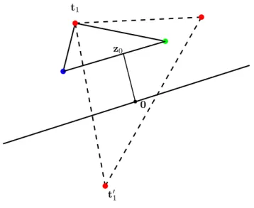
Consider d + 1 sets of points S1, . . . , Sd +1inRd such that 0 ∈Td +1i =1 conv(Si). Consider
now a colorful set T = {t1, . . . , td +1} that is closest to 0. By closest, we mean a colorful
set T minimizing dist¡0,conv(T )¢. If dist¡0,conv(T )¢ = 0, then 0 ∈ conv(T ), and hence T satisfies the statement of the theorem. Otherwise, consider a point z0∈ conv(T )
1.3. Proofs of the colorful Carathéodory theorem
minimizing kz0k2. For all z ∈ conv(T ), we have zT0z > 0. Besides, z0can be written as a
positive sum of points in T , namely z0=Pd +1i =1 γiti, withγi ≥ 0 for all i ∈ [d +1] and one
of theγi’s equal to 0. Indeed, if conv(T ) is a simplex of dimension d , the projection
of 0 lies on a face of the simplex, and if conv(T ) is of smaller dimension, then we can clearly set one of theγi’s to zero.
Without loss of generality, we assume thatγ1= 0. Since t1∈ conv(T ), we have zT0t1> 0.
Since 0 ∈ conv(S1), there is necessarily a vector t01∈ S1such that zT0t01< 0. Replacing t1
by t01in T we obtain a colorful set T0, which is strictly closer to 0 than T. Indeed, for 0 ≤ α ≤ 1, we have (1 − α)z0+ αt01∈ conv(T0), and
dist(0, T0)2≤ k(1 − α)z0+ αt01k 2
= (1 − α)2kz0k2+ 2α(1 − α)zT0t01+ α2kt10k2.
Choosingα > 0 small enough, we obtain dist(0,T0) < dist(0,T ). This contradiction shows that T must contain 0 in its convex hull.
b 0 z0 b b b b b t1 t′ 1
Figure 1.1: Bárány’s proof of the colorful Carathéodory theorem
This proof provides an algorithm for finding a colorful set containing 0 in its convex hull. The algorithm goes roughly as follows. Choose a colorful set T . As long as T does not contain 0 in its convex hull, we can replace one point of T as in the previous proof and obtain a colorful set strictly closer to 0. Since there is a finite number of colorful sets, this algorithm ends and returns a positively dependent colorful set. This algorithm is not known to be polynomial and has been studied in [5] and later in [18]. We discuss it more thoroughly in Section 2.1.2.
1.3.2 Sperner’s lemma proves the colorful Carathéodory theorem
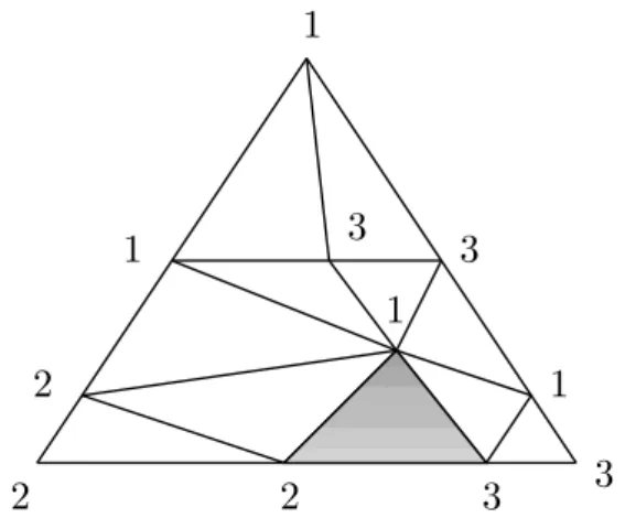
We sketch here a new proof of Theorem 1.2.3, and hence of the strong version of the colorful Carathéodory theorem, namely Theorem 1.2.4. The proof uses the well-known Sperner’s lemma, originally introduced to give a constructive proof of the Brouwer fixed point theorem [49]. The motivation for this proof is to make a connection between two colorful results.Consider a d -simplex∆d = conv{v1, . . . , vd +1}, and a triangulationTof this simplex. A
Sperner labeling is a mapλ : V (T) → [d+1] such that for v ∈ V (T), ifF = conv(vi1, . . . , vik)
is the smallest face of∆d containing v, thenλ(v) ∈ {i1, . . . , ik}. In particular, we have
λ(vi) = i for all i ∈ [d + 1].
A simplex in the triangulation is fully-labeled if it is of dimension d and its vertices have pairwise distinct labels.
1 2 3 3 3 1 3 1 1 2 2
Figure 1.2: A Sperner labeling in dimension 2
Theorem 1.3.1 (Sperner’s Lemma, Sperner [49]). Given a triangulated simplex and a Sperner labeling of its triangulation, there exists an odd number of fully-labeled simplices.
The proof of this theorem is standard and may be found in [13,48].
Given a polyhedronP = ©x ∈ Rn| Ax = b, x ≥ 0ª and a set I ⊆ [n], we define a polyhe-dronPI :=©x ∈ P | xi = 0 for all i ∉ Iª. If A is of full rank, the dimension ofPI is at
most |I | − d, for |I | ≥ d. The faces of P are exactly the PI’s, with I ⊆ [n] (the empty
face being considered as one of the faces).
Consider now A, b, and disjoint feasible bases B1, . . . , Bd as in the statement of
1.3. Proofs of the colorful Carathéodory theorem
b | x ≥ 0ª is non-degenerate. We defineP to be the polyhedron P := ©x ∈ Rn|Ax = b, x ≥ 0ª. The vertices ofP are identified with the feasible bases B ⊆ [n]. Define a labelingλ of the vertices of the polyhedron by
λ(B) := min argmaxi ∈[d]¡|B ∩ Bi|¢.
Less formally, the label of a vertex identified with B is the index i maximizing |B ∩ Bi|.
If there is more than one such i , thenλ(B) is chosen as the smallest among them. In particular, we haveλ(Bi) = i .
Consider now B1and B2. Because of the connectedness of the 1-skeleton of the face
PB1∪B2, there is a path between the two vertices B1and B2in this graph. The vertices on this path correspond to bases B ⊆ B1∪ B2, and hence having their labels equal
to 1 or 2. Similarly, we define a path between B1and B3and a path between B2and
B3. Again, by a connectedness argument, these three paths form the boundary of a
polyhedral complex on the boundary of the facePB1∪B2∪B3 of dimension 2. All the vertices of this complex clearly have their labels equal to 1, 2, or 3.
In general, given a set X ∈ [d], we defineRX to be a polytopal complex of dimension
|X | − 1 whose boundary is ∂RX =Si ∈XRX \{i }. Such a complex exists, since the face
PS
i ∈XBi is connected. In the end, we have a polyhedral complex K=R[d ] on the
boundary ofP , whose polyhedra are of dimension at most d − 1. Furthermore, this polyhedral complex resembles the faces of ∆d with the identfication “RX ∼= face of
∆d”. The labeling of this complex is a proper labeling for Sperner’s lemma. Up to
triangulating the polyhedra inK, we have thus at least one fully-labeled (d −1)-simplex, and hence at least one fully-labeled faceF of P of dimension d − 1, i.e. a face such thatλ(V (F )) = [d].
Recall that a face ofP is a polyhedron PI for some I ⊆ [n]. Considering I minimal
such that the face is equal toPI, the dimension of the face is at least |I | − d. Hence, we
have found a set I ⊆ [n] such that |I | ≤ 2d − 1 and such that all possible labels are used on the vertices ofF . Thus, we have Bi∩ I 6= ; for all i ∈ [d] and hence |Bi∩ I | = 1 for
some i ∈ [d]. Consider such a i , and call it i0. Let B be a feasible basis associated with
a vertex ofF whose label is i0. We have |B ∩ Bi| ≤ |B ∩ Bi0| = 1 for all i ∈ [d]. Therefore, B is a colorful feasible basis, which proves the theorem.
There is an algorithmic proof of Sperner’s lemma. Therefore, this new proof gives, in some sense, another algorithm for the colorful Carathéodory theorem. Here again we do not know the exact complexity but it might be exponential.
1.4 Applications in geometry
This section gathers applications of the colorful Carathéodory theorem in discrete geometry.
1.4.1 Tverberg’s theorem
Given a set S of n points inRd, a Tverberg k-coloring of S is a partition of the points in S into k sets S1, . . . , Sksuch thatTki =1conv(Si) is nonempty. Tverberg’s theorem, proved
in 1966 [52], states the following.
Theorem 1.4.1(Tverberg’s theorem). Any set of n points inRd with n ≥ (k −1)(d +1)+1 admits a Tverberg k-coloring.
Sarkaria proposed a proof of this theorem using the colorful Carathéodory theorem [46]. We present here a simplified version of this proof by Bárány and Onn [5].
Proof. Consider a finite set S = {v1, . . . , vn} ⊆ Rd and an integer k such that n ≥ (k −
1)(d + 1) + 1. Let N = (k − 1)(d + 1). A Tverberg k-coloring of the points in {v1, . . . , vN +1}
induces a Tverberg k-coloring of S, by assigning the remaining points in S to any set of the partition. We can thus assume that n = N + 1. The idea of the proof is to define k copies of each point in S, numbered from 1 to k, in a space of higher dimension. A colorful set in this higher dimensional space will associate each point of S to one of its k copies, and hence will give a partition of S.
Choose arbitrarily a family f1, . . . , fk∈ Rk−1such that f1+ · · · + fk= 0, and such that any
subfamily is linearly independent. For i ∈ [n], define the set of k copies of vi by
Ti = n fj⊗ Ã vi 1 ! | j ∈ [k] o ⊆ Rk−1⊗ Rd +1.
We clearly have 0 ∈ conv(Ti) for all i ∈ [n]. Applying the colorful Carathéodory theorem,
in dimension N , to the colors T1, . . . , TN +1, we obtain a colorful set T =
n fπ(i)⊗ Ã vi 1 ! | i ∈ [N + 1]ocontaining 0 in its convex hull, whereπ(i) ∈ [k] is the index j of the point of Ti
chosen in T . We have 0 =Pn i =1αifπ(i)⊗ Ã vi 1 !
, withα ≥ 0, which can be rewritten
0 = k X j =1 X i ∈π−1( j ) αifj⊗ à vi 1 ! = k X j =1 fj⊗ à X i ∈π−1( j ) αi à vi 1 !! .
1.4. Applications in geometry
Thus, by the assumption made on the fi’s, we have
X i ∈π−1(1) αi à vi 1 ! = · · · = X i ∈π−1(k) αi à vi 1 ! . Let M = P
i ∈π−1(1)αi = · · · =Pi ∈π−1(k)αi and define Sj :=©vi ∈ S | i ∈ π−1( j )ª for all j ∈ [k]. We have
z = 1 M
X
i ∈π−1(1)
αivi∈ conv(Sj), for all j ∈ [k].
We conclude that the partition S1, . . . , Skdefines a Tverberg k-coloring of S.
1.4.2 First selection lemma
Given n points in the plane in general position, a result by Boros and Füredi [8] states that there is a point, not necessarily one of these n points, in at least 29¡n
3¢ triangles
spanned by these points, and that this is the best possible bound. A similar statement holds in arbitrary dimension, answering a question of Boros and Füredi. It was first proved by Bárány as an application of the colorful Carathéodory theorem.
Theorem 1.4.2 (First selection lemma). Given a set S of n points in Rd in general position, there exists a point p ∈ Rd contained in at least cd
¡ n
d +1¢ simplices of dimension
d formed by points of S, where cd is a constant depending only on the dimension d .
The proof by Bárány provides a constant cd equal to (d + 1)−(d+1). A better bound was
obtained by Gromov [23,28] via a topological approach providing a constant cd equal
to (d +1)!1 .
Proof of Theorem 1.4.2. The proof starts by using Tverberg’s theorem to partition the points in S. Define k :=¥n−1d +1¦ + 1 such that |S| ≥ (k − 1)(d + 1) + 1. We assume that n is sufficiently large, so that k > d. According to Tverberg’s theorem, we have a partition of S into k sets, or colors, S1, . . . , Sksuch thatTki =1conv(Si) is nonempty.
Up to translating the configuration, we can assume that 0 ∈Tk
i =1conv(Si). Apply the
colorful Carathéodory theorem for every choice of d + 1 sets Si1, . . . , Sid +1among the k
colors. It gives a positively dependent colorful set. Besides, each choice of Si1, . . . , Sid +1
provides a different colorful set. Therefore 0 is in at least¡d +1k ¢ =(d +1)1d +1¡d +1n ¢ +O(nd) simplices.
1.4.3 Weak
ε-nets
Given a set X ⊆ Rd in general position with |X| = n, and ε > 0, the set S ⊆ Rd is a weak ε-net if it satisfies S ∩ conv(Y) 6= ; for all Y ⊆ X of size |Y| ≥ εn. The problem here is to find a weakε-net as small as possible. Applying the first selection lemma, we can show the following theorem, better bounds have been obtained by Chazelle et al. [10].
Theorem 1.4.3. Given a set of points X ⊆ Rd in general position with |X| = n, there exists a weakε-net of size at most O¡ 1
cdεd +1¢.
Proof of Theorem 1.4.3. Start with S = ; and H =¡ X
d +1¢. At each step, ask whether
there is a subset Y ⊆ X such that |Y| ≥ εn and S∩conv(Y) = ;. If the answer is no, then S is a weakε-net and return it. Otherwise, consider such a Y. Applying the first selection lemma, there is a point z in the convex hull of at least cd
¡ |Y|
d +1¢ simplices formed by
points of Y. Let S := S ∪ {z} and H = H \ {T ∈ H | z ∈ conv(T)}. The initial setH is of size ¡ n
d +1¢ and at each step, at least cd
¡εn
d +1¢ elements ofH are
removed from it. Hence, there is at most O¡ 1
cdεd +1¢ steps, and in the end, the set S is a
weakε-net of size at most O¡ 1
cdεd +1¢.
1.5 Octahedron lemma: three proofs
The following lemma is ubiquitous in colorful linear programming.
Theorem 1.5.1 (Octahedron lemma). Consider d + 1 pairs of points S1, . . . , Sd +1inRd
and a point p ∈ Rd, all together in general position. The point p is contained in an even number of colorful simplices.
In dimension 2, it means that given two blue points, two red points, and two green points in the plane, in general position, any point in the plane is covered by an even number of colorful triangles, see Figure 1.3.
This theorem has a similar flavor as the colorful Carathéodory theorem, and leads to similar algorithmic questions, studied in Chapter 2. It is also a key tool for counting the number of colorful simplices under the conditions of the colorful Carathéodory theorem, see Chapter 4 and Chapter 5.
We propose three different proofs of the Octahedron lemma. Although this theorem was known and used in [4,18,19], the proof was not fully written before 2011 [41].
1.5. Octahedron lemma: three proofs b b b b b b b p
Figure 1.3: The Octahedron lemma in dimension 2
1.5.1 Topological proof
The first proof is topological and was mentioned by Bárány and Matoušek [4].
Topological proof of Theorem 1.5.1. Consider the crosspolytope3d +1inRd +1, i.e. the polytope whose vertices are e1, −e1, . . . , ed +1, −ed +1, with ei the standard i th unit vector.
Define a mapping from3d +1toRd, by mapping ei and −ei to the two points in Si for
all i ∈ [d + 1], and extend it affinely, see Figure 1.4
By a basic topological argument, each point ofRd has an even number of points in its preimage, except those that are the image of points in the faces of3d +1of dimension d − 1. Since the facets of3d +1are exactly mapped to the colorful simplices inRd and since S1, . . . , Sd +1and p are in general position, the point p is in an even number of
colorful simplices.
1.5.2 Parity proof argument
The following proof was proposed by Meunier and Deza [41].
Proof of Theorem 1.5.1 using complementary pivots. Consider d + 1 pairs of points S1,
. . . , Sd +1 inRd and a point p ∈ Rd in general position. Define a graph G = (V,E) as follows. The vertices in V are identified with subsets ofSd +1
i =1 Si. We consider three
types of subsets, defining three sets of vertices V1, V2, and V3. The vertices in V1
b b b b b b b b b b b b
Figure 1.4: Affine mapping of the crosspolytope
correspond to sets T ⊆Sd +1
i =1 Si such that |T ∩ Si| ≤ 1 for all i ∈ [d], Sd +1⊆ T , |T | ≤ d + 1,
and p ∈ conv(T ). Note that since the points are in general position, the vertices in V1
and V2correspond to sets of size d + 1. Hence, the vertices in V2correspond to sets
missing exactly one color. Finally, the vertices of V3correspond to sets T such that
|T ∩ Si| ≤ 1 for all i ∈ [d], Sd +1⊆ T , |T | = d + 2, and p ∈ conv(T ).
Two vertices are neighbors in G if one of them is in V1∪ V2and the other is in V3, and if
the corresponding sets have d + 1 points in common. We show that the vertices in V1
are of degree 1, and that the vertices in V2and V3are of degree 2. The graph G being a
collection of cycles and paths with endpoints in V1, we conclude that |V1| is even.
Consider a vertex v ∈ V3and the corresponding set T . The neighbors of v correspond
to sets T0⊆ T such that |T0| = d + 1 and p ∈ conv(T0). By a usual argument in linear programming, there are exactly two of them. Consider a vertex v ∈ V1and the
corre-sponding set T . It is clear that v has exactly one neighbor, which is the vertex of V3
corresponding to T ∪ Sd +1. Finally, consider v ∈ V2and the corresponding set T . It
misses one color Sj= {s1j, s2j}, and hence v has exactly two neighbors being the vertices
1.5. Octahedron lemma: three proofs
1.5.3 Geometric proof
The following proof was inspired by discussions with Raman Sanyal on the combinato-rial proof of the colorful simplicial depth conjecture, see Chapter 4.
Geometric proof of Theorem 1.5.1. Consider d + 1 pairs of points S1, . . . , Sd +1inRdand
a point p ∈ Rd in general position. For each transversal T ⊆Sd +1
i =1Si, consider the
(d − 1)-simplex defined by conv(T ). Denote byKthe sets of all these simplices. Pick a point p0∈ Rd not in conv(Sd +1i =1 Si). The point p0is in no colorful simplices. Consider
the line L joining p0and p. Up to slightly moving the point p0, we can assume that this
line crosses the simplices inKin their interior and on distinct points. We denote by T1, . . . , Tr the transversals corresponding to the simplices ofKintersected by L in this
order when going from p0to p, and by q1, . . . , qr the intersection points.
Clearly no colorful simplices contain a point in [p0, q1[. All points in ]qi, qi +1[ are
contained in exactly the same colorful simplices, for i ∈ [r − 1], and all the points in ]qr, p] are contained in exactly the same colorful simplices.
We denote byΩ0the empty-set, by Ωi the set of colorful simplices containing the
points in ]qi, qi +1[ for i ∈ [r − 1], and by Ωr the set of colorful simplices containing
the points in ]qr, p]. Note thatΩr is exactly the set of colorful simplices containing
p. Finally, for a transversal T , we note U (T ) the set of all colorful simplices having conv(T ) as a facet. We have |U (T )| = 2, since the Si’s are all of size 2.
Note thatΩi +1= Ωi4U (Ti), where 4 denotes the symmetric difference (defined for
two sets A and B by A4B = (A ∪ B) \ (A ∩ B)). Since |Ω0| = 0 and |U (Ti)| = 2 for all
i ∈ [r ], we have that |Ωi| is even for all i ∈ [r ]. In particular, |Ωr| is even.
Considering more generally the Si’s being of even size, instead of being simply pairs,
we get the following theorem with an almost identical proof. This theorem was given in [20].
Theorem 1.5.2 (Extension of the Octahedron lemma). Consider d + 1 sets of points S1, . . . , Sd +1inRd and a point p ∈ Rd, all together in general position. If |Si| is even for
all i ∈ [d + 1], then the point p is covered by an even number of colorful simplices.
We now show that Theorems 1.5.1 and 1.5.2 are equivalent. It is clear that Theorem 1.5.2 implies the Octahedron lemma. The converse is also true: we can prove Theorem 1.5.2 from the Octahedron lemma.
Proof. Consider d + 1 sets S1, . . . , Sd +1, with |Si| even for all i ∈ [d + 1] and a point
p ∈ Rd in general position. For any X = X1∪ · · · ∪ Xd +1 with Xi ⊆ Si and |Xi| = 2 for
all i , define N (X) to be the number of colorful simplices, formed with points in X, containing p. Let N be the total number of colorful simplices containing p. We haveP
XN (X) = NQd +1i =1(|Si| − 1), since every colorful simplex containing p is counted
Qd +1
i =1(|Si| − 1) times in this sum. The Octahedron lemma ensures that N (X) is even for
all X. SinceQd +1
i =1(|Si| − 1) is odd, N is also even.
1.6 Other colorful results in geometry
We end this chapter with two colorful results in geometry, more or less related to the colorful Carathéodory theorem.
1.6.1 Colored Tverberg’s theorem
Given d + 1 sets of points S1, . . . , Sd +1inRd, the problem, known as colored Tverberg,
aims at finding a point in the convex hulls of many disjoint colorful sets. For d , r ∈ Z+
we define t (d , r ) to be the minimal integer, independent from the Si’s, such that if
|Si| ≥ t (d, r ) for all i , then there are r disjoint colorful sets whose convex hulls intersect.
The following colored Tverberg theorem was conjectured by Bárány, Füredi, and Lovász in 1990 [6].
Theorem 1.6.1. t (d , r ) is finite for all d , r ∈ Z+.
A proof of t (d , 2) = 2 was first given by Lovász. His proof can be found in a paper by Bárány and Larman [3], in which they also proved that t (1, r ) = t(2,r ) = r , and conjectured that t (d , r ) = r for all d,r ∈ Z+.
The general case was first proved by Živaljevi´c and Vre´cica [54], who also showed that for r prime, we have t (d , r ) ≤ 2r − 1. Later Blagojevi´c, Matschke, and Ziegler proved that for r + 1 prime, we have t(d,r ) = r , via a topological proof [7]. The conjecture of Bárány and Larman remains open.
1.6.2 Colorful Helly’s theorem
The second result we present here, known as colorful Helly theorem, was introduced by Lovász and presented by Bárány in 1982, in his paper on the colorful Carathéodory theorem [2].
1.6. Other colorful results in geometry
Theorem 1.6.2 (Colorful Helly’s theorem, Lovász [2]). LetF1, . . . ,Fd +1be d + 1 finite
families of convex sets inRd. If for all choices of d + 1 sets F1∈ F1, . . . , Fd +1∈ Fd +1, we
haveTd +1
i =1Fi6= ;, then
T
F ∈FiF 6= ; for some i ∈ [d + 1].
The usual Helly theorem, states that, given a family of n convex sets, if every d + 1 of them intersect, then they all intersect. This result is a corollary of Theorem 1.6.2, by takingF1= · · · = Fd +1.
The key tools used by Bárány for proving Theorem 1.6.2 are the classical Helly theorem and the colorful Carathéodory theorem.