Dégradation des aspérités des joints rocheux sous différentes conditions de chargement

(1)

Département de génie civil

DÉGRADATION DES ASPÉRITÉS DES JOINTS

ROCHEUX SOUS DIFFÉRENTES CONDITIONS DE

CHARGEMENT

Thèse de doctorat Spécialité : Génie Civil

Ali FATHI

Jury : Patrice RIVARD (directeur) Gérard BALLIVY

Giovanni GRASSELLI Ali SAEIDI

Baptiste ROUSSEAU

(2)

(3)

À ma mère, à mon père et à ma femme bien-aimée, de soutien à l'infini

“

ETUDIE, NON POUR SAVOIR PLUS, MAIS POUR SAVOIR MIEUX

”

Sénèque

(4)

(5)

i

L’objectif de cette thèse est d’interpréter la dégradation des aspérités des joints rocheux sous différentes conditions de chargement. Pour cela, la variation des aspérités durant les différentes étapes du cisaillement d’un joint rocheux est observée. Selon le concept appelé “tiny windows”, une nouvelle méthodologie de caractérisation des épontes des joints a été développée. La méthodologie est basée sur les coordonnées tridimensionnelles de la surface des joints et elles sont mesurées après chaque essai. Après la reconstruction du modèle géométrique de la surface du joint, les zones en contact sont identifiées à travers la comparaison des hauteurs des “tiny windows” superposées. Ainsi, la distribution des zones de la surface en contact, endommagées et sans contact ont été identifiées. La méthode d’analyse d’image a été utilisée pour vérifier les résultats de la méthodologie proposée. Les résultats indiquent que cette méthode est appropriée pour déterminer la taille et la distribution des surfaces du joint en contact et endommagées à différentes étapes du cisaillement.

Un ensemble de 38 répliques ont été préparées en coulant du mortier sans retrait sur une surface de fracture obtenue à partir d’un bloc de granite. Différentes conditions de chargement, incluant des chargements statiques et cycliques ont été appliquées afin d’étudier la dégradation des aspérités à différentes étapes du procédé de cisaillement. Les propriétés géométriques des “tiny windows” en contact en phase pré-pic, pic, post-pic et résiduelle ont été analysées en fonction de leurs angles et de leurs auteurs. Il a été remarqué que les facettes des aspérités faisant face à la direction de cisaillement jouent un rôle majeur dans le cisaillement. Aussi, il a été observé que les aspérités présentent différentes contributions dans le cisaillement. Les aspérités les plus aigües (“tiny windows” les plus inclinées) sont abîmées et les aspérités les plus plates glissent les unes sur les autres. Les aspérités d’angles intermédiaires sont définies comme “angle seuil endommagé” et “angle seuil en contact”. En augmentant la charge normale, les angles seuils diminuent d’une part et, d’autre part, le nombre de zones endommagées et en contact augmentent. Pour un petit nombre de cycles (avec faible amplitude et fréquence), indépendamment de l’amplitude, une contraction apparaît ; par conséquent, la surface en contact et les paramètres de résistance au cisaillement augmentent légèrement. Pour un grand nombre de cycles, la dégradation est observée à l’échelle des aspérités de second ordre, d’où une baisse des paramètres de résistance au cisaillement. Il a été aussi observée que les “tiny windows” avec différentes inclinaisons contribuent au processus de cisaillement, en plus des “tiny windows” les plus inclinées (aspérités plus aigües). Les résultats de la méthode proposée montrent que la différenciation entre les zones en contact et celles endommagées s’avère utile pour une meilleure compréhension du mécanisme de cisaillement des joints rocheux.

Mots-Clés: Joint rocheux; Mécanisme de cisaillement; Aspérités; Rugosité; Aire de contact; Aire

(6)

(7)

iii

The objective of the current research is to interpret the asperity degradation of rock joints under different loading conditions. For this aim, the changes of asperities during different stages of shearing in the three-dimensional joint surface are tracked. According to a concept named ‘tiny window’, a new methodology for the characterization of the joint surfaces was developed. The methodology is based on the three-dimensional coordinates of the joints surface that are captured before and after each test. After the reconstruction of geometric models of joint surface, in-contact areas were identified according to the height comparison of the face to face tiny windows. Therefore, the distribution and size of just in-contact areas, in-contact damaged areas and not in-contact areas are identified. Image analysis method was used to verify the results of the proposed method. The results indicated that the proposed method is suitable for determining the size and distribution of the contact and damaged areas at any shearing stage.

A total of 38 replicas were prepared by pouring non-shrinking cement mortar on a fresh joint surface of a split granite block. Various loading conditions include monotonic and cyclic loading were applied to study the asperities degradation at different stages of shearing. The geometric properties of the in-contact tiny windows in the pre-peak, peak, post-peak softening and residual shearing stages were investigated based on their angle and height. It was found that those asperities facing the shear direction have the primary role in shearing. It is remarkable that different part of these asperities has their own special cooperation in shearing. The steepest parts (steeper tiny windows) are wore and the flatter parts (flatter tiny windows) are slid. The borderlines between these tiny windows defined as “damaged threshold angle” and “in-contact threshold angle”.

By increasing normal load, both the amounts of threshold angles are decreased and contact and damaged areas increased. During low numbers of cycles (with low amplitude and frequency), independent of the type of cycle, contraction occurs and consequently the contact area and the shear strength parameters slightly increased. During larger number of cycles, degradation occurred on the second order asperities, therefore the shear strength parameters slowly decreased. It was also observed that tiny windows with different heights participate in the shearing process, not just the highest ones. The results of the proposed method indicated that considering differences between just in-contact areas and damaged areas provide useful insights into understanding the shear mechanism of rock joints.

Keywords: Rock joints; Shear Mechanism; Asperities; Roughness; Contact Areas; Damaged Areas;

(8)

(9)

v

Among many people who helped me to complete this thesis, first I want to express my sincere gratitude to my supervisor, Professor Patrice Rivard, for his guidance throughout the duration of the study. I am greatly indebted for his support, advice, and suggestions to my research work. I would like to thank my co-supervisor, Professor Gérard Ballivy, for his great assistance and his guidance during various parts of the work. Dr. Zabihallah Moradian has assisted me with many interesting discussions and comments. He is greatly acknowledged. I thank Dr. Clermont Gravel for his support and many inspirations and also for his useful comments.

I would like to express my thanks to Prof. Giovanni Grasselli, Prof. Ali Saeidi, Dr. Baptiste Rousseau and Prof. Mathieu Nuth for evaluating my thesis and giving their useful comments and suggestions.

Gratitude is also expressed to those working at Laboratory of Rock Mechanics and Applied Geology, Civil Engineering Department, Université de Sherbrooke especially, Georges Lalonde, Danick Charbonneau and Ghislaine Luc who have helped me to carry out laboratory tests.

There are many colleagues and friends who deserve my sincere gratitude and acknowledgements. I thank all of them for their encouragement in various ways. I am so grateful that I have come to know and make friends with these wonderful People during my graduate study.

I want to thank my family and especially my parents, because their support has been invaluable. Finally, special thanks to my beloved wife who made this work possible with her patience and support.

(10)

(11)

TABLE OF FIGURES

Figure 1.1 Frank slide area, Alberta, Canada [from Marek Ślusarczyk, 2007]. ... 2 Figure 1.2 The Hope slide area, Hope, BC, Canada [from Magnus Manske, 2005]. ... 2 Figure 1.3 St. Francis dam almost 2 years before and 5 days after the collapse [Photos from C.H. Lee Collection, U.C. Water Resources Center Archives, colorized by Pony Horton]... 3 Figure 1.4 Malpasset concrete dam before (Bureau COB 1954) and after collapse [from Eolefr, 2014]. 3 Figure 1.5 Vajont Dam Before and After Failure [Tzamtzis et Asteris, 2004]... 4 Figure 1.6 Schematic test setup - direct shear box with encapsulated specimen [ASTM D5607 – 08]. .. 5 Figure 1.7 Typical results of direct shear tests on a tension fracture [after Barton, 1976]. ... 5 Figure 1.8 Bilinear failure envelope proposed by Patton [1966]. ... 7 Figure 1.9 Ladanyi et Archambault's [1970] frictional work components. ... 9 Figure 1.10 Shear displacement-dilation response and stress path plot for 12.5 ~ regular triangular asperities joint in Johnstone [Seidel et Haberfield, 1995]. ...10 Figure 1.11 Deformations due to inelasticity [Seidel et Haberfield, 1995]. ...11 Figure 1.12 Roughness profiles and corresponding JRC values [after Barton et Choubey, 1977]. ...12 Figure 1.13 Reduction of asperity contact area with progressive shear displacement and local normal stress increases [Seidel et Haberfield, 2002]. ...13 Figure 1.14 Geometrical identification of the apparent dip angle in function of the shear direction [Grasselli, 2001]. ...15 Figure 1.15 Shear strength model parameters: (a) typical cyclic shear curve showing the four portions; (b) morphological parameters [Belem et al., 2004]. ...16 Figure 1.16 Cyclic shear behavior of smooth (top photo) and rough (bottom photo) joints [Lee et al., 2001]. ...20 Figure 1.17 Shear stress–shear displacement curve of small cyclic displacement and large cyclic displacement [Jafari et al., 2003]. ...21 Figure 1.18 Range of boundary conditions across a joint surface. ...24

(16)

Figure 1.19 Shear stress vs. shear displacement models (a) Constant stiffness model, (b) Constant displacement model [after Goodman, 1976]. ...24 Figure 2.1 Manufacturing of the mortar replicas b) Diagram of SIKA grading test. ...36 Figure 2.2 The effect of 3 sampling intervals on the roughness parameters and profile reconstruction. 37 Figure 2.3 Roughness parameters defined in 2D ( Z2 and Rp) and 3D (RS). ...39

Figure 2.4 Values of Z2 (left) and Rp (right) calculated for different directions (Specimen A127) with 0.5 mm intervals. The zero direction is parallel to the shear direction. ...40 Figure 2.5 MTS press system b) Diagram of vertical section of the shear apparatus. ...41 Figure 2.6 Joint surface divided into a large number of tiny windows. The tiny windows size will vary depending on the accuracy required. ...42 Figure 2.7 a) upper surface and lower surface were defined in the same coordinate system. b) the upper surface was meshed with the same interval as the lower surface. ...44 Figure 2.8 Some targets were attached around the shear box and were scanned with the joint surface. 45 Figure 2.9 Assessment criteria for contact condition; a) zero = tiny windows are just in-contact, b) positive = tiny windows are not in contact c) negative = these windows are in contact and damaged and degradation has occurred. Total contact area is the sum of just in-contact areas and in-contact damaged areas. ...46 Figure 2.10 Distribution and amount of tiny windows angles with respect to the shear direction before shear test (the total number of tiny windows - 0.2 × 0.2 mm - is 490000). ...47 Figure 2.11 Frequency plot of the height and angle of the tiny windows. ...48 Figure 2.12 Shear stress and dilation versus shear displacement for Specimen A127 under 0.8 MPa normal stress. ...49 Figure 2.13 Anticipated results using the proposed method a) total contact areas (TCA), black spots and b) cumulative damaged areas (colored spots) occurring during shear tests after 1) 0.2, 2) 1 and 3) 10 mm shear displacements (SD). ...49 Figure 2.14 Shear stress and dilation vs shear displacement at 0.2, 1 and 10 mm shear displacements. 52 Figure 2.15 Distribution of the damaged areas (black spots) occurred during shear test after a) 0.2, b) 1 and c) 10 mm shear displacements with image analysis method. ...52 Figure 2.16 Shear stress and dilation versus shear displacement for shear tests under different levels of normal stress. ...53

(17)

Figure 2.17 The contact area was calculated by considering the angle of each tiny window and the

number of tiny windows for each increment. ...54

Figure 2.18 Frequency of in-contact tiny windows area versus their angle, under 0.1 MPa normal stress after a) 0, b) 0.2, c) 0.4, d) 1, e) 6 and f) 10 mm shear displacements. ...55

Figure 2.19 Frequency of in-contact tiny windows area versus their angle, under 0.7 MPa normal stress after a) 0, b) 0.2, c) 0.4, d) 1, e) 6 and f) 10 mm shear displacements. ...56

Figure 2.20 The top of some asperities sheared and tiny windows that were not initially facing the shear direction (negative angles) changed into tiny windows that are facing the shear direction (positive angles). ...57

Figure 2.21 In-contact damaged area and just in-contact area versus shear displacement under 0.1 and 0.7 MPa normal stresses. ...59

Figure 2.22 Total contact area versus shear displacement under different normal stresses from 0.1 to 0.7 MPa. ...60

Figure 2.23 Frequency of in-contact tiny windows versus their heights under 0.1 MPa normal stress and after different shear displacements. ...61

Figure 2.24 Frequency of in-contact tiny windows versus their heights under 0.7 MPa normal stress and after different shear displacements. ...62

Figure 2.25 Frequency histogram of in-contact tiny windows by considering their heights and angles simultaneously. ...64

Figure 2.26 Frequency of the in-contact tiny windows after a) 0, b) 0.2, c) 0.4, d) 1, e) 6 and f) 10 mm shear displacements and under 0.1 MPa normal stress by considering their heights and angles...65

Figure 2.27 Frequency of the in-contact tiny windows after a) 0, b) 0.2, c) 0.4, d) 1, e) 6 and f) 10 mm shear displacements and under 0.7 MPa normal stress by considering their heights and angles...66

Figure 3.1 Manufacturing of the mortar specimens. ...75

Figure 3.2 MTS press system b) Diagram of vertical section through shear apparatus. ...76

Figure 3.3 Scanner set up. ...76

Figure 3.4 Joint surface divided into a large number of tiny windows [Fathi et al., 2015]...78

Figure 3.5 The joint surface of Specimen A115 was characterized using new methodology a) topography and b) angle distribution plots. ...79

Figure 3.6 Shear stress and dilation versus shear displacement for a monotonic shear test under 0.8 MPa normal stress. ...80

(18)

Figure 3.7 Cyclic shear tests subjected to 5, 10, 20, 100, 500 and, 1000 cycles and amplitude of cycles of 30%. ...83 Figure 3.8 Cyclic shear tests subjected to 100, 500 and, 1000 cycles and amplitude of cycles of 50%. 85 Figure 3.9 Frequency of in-contact tiny windows area versus their angle after cyclic loading at 0.2 mm shear displacement when the amplitude of cycles was 30%. a) Initial stage of shearing b) monotonic test c) after 5 cycles d) after 10 cycles e) after100 cycles g) after 500 cycles and h) after 1000 cycles. 87 Figure 3.10 The total contact area at 0.2 mm shear displacement increased from 46.2% to 62.1% when number of cycles increased from a) 5 cycles to b) 1000 cycles. The amplitude of cycles was 30%. ...88 Figure 3.11 Frequency of in-contact tiny windows after cyclic loading at 0.2 mm shear displacement when the amplitude of cycles was 50%. a) after 0 cycles b) after 100 cycles c) after 500 cycles and d) after 1000 cycles. ...89 Figure 3.12 Shear displacements and dilations at the end of cycles (load-controlled stage) vs number of cycles...90 Figure 3.13 Total contact area and dilation vs. number of cycles after cyclic loading stage of shearing at 0.2 mm shear displacement when the amplitude of cycles was a) 30% and b) 50%...91 Figure 3.14 Peak and residual shear strength versus number of cycles for pre-peak cyclic loading tests with amplitude of a) 30% and b) 50%...92 Figure 3.15 Distribution of contact areas and frequency of in-contact tiny windows at a) initial stage of shearing and after b) 0 cycles (monotonic test) c) 5 cycles d) 10 cycles e) 20 cycles f) 100 cycles g) 500 cycles and h) 1000 cycles of loading at 0.4 mm shear displacement when the amplitude of cycles was 30%. ...93 Figure 3.16 The total contact area at 0.4 mm shear displacement increased from 24.5% to 26.4% when number of cycles increased from a) 5 cycles to b) 1000 cycles. The amplitude of cycles was 30%. ...94 Figure 3.17 Distribution of contact areas and frequency of in-contact tiny windows after a) 0 cycles b) 100 cycles c) 500 cycles and d) 1000 cycles at 0.4 mm shear displacement when the amplitude of cycles was 50%. ...95 Figure 3.18 Total contact area and dilation at 0.4 mm shear displacement vs. number of cycles. ...96 Figure 4.1 Interface shear stress in the upstream side of the Long Spruce Dam on the Nelson River in the northeast of Canadian province of Manitoba [Zhang, 1998]. ... 102 Figure 4.2 Hourly time series plots of principal stress amplitudes [Prinsenberg et al., 1997]. ... 102 Figure 4.3 Four types of loading-unloading conditions. ... 106

(19)

Figure 4.4 Joint surface divided into a large number of tiny windows. Each tiny window represents the height and angle of a small area of the joint surface [Fathi et al., 2015a]. ... 107 Figure 4.5 The joint surface of Specimen A125 was characterized using new methodology a) frequency of tiny windows based on their heights and topography plot and b) frequency of tiny windows based on their angles and angle distribution plot. ... 107 Figure 4.6 a) Shear stress and dilation versus shear displacement for type 1 loading-unloading test, b) a close-up of the unloading part, and c) shear stress and dilation versus time for the loading-unloading part. ... 109 Figure 4.7 Stiffness and dilation versus number of cycles of loading-unloading tests (Specimen A124). ... 109 Figure 4.8 a) Shear stress and dilation versus shear displacement for type 2 loading-unloading test, b) a close-up of the unloading part, and c) shear stress and dilation versus time for the loading-unloading part. ... 110 Figure 4.9 Stiffness and dilation versus number of type 2 loading-unloading cycles (Specimen A114). ... 111 Figure 4.10 Shear stress and dilation versus shear displacement for type 3 loading-unloading test, b) a close-up of the unloading part, and c) shear stress and dilation versus time for the loading-unloading part. ... 111 Figure 4.11 Stiffness and dilation versus number of cycles for type 3 loading-unloading test (Specimen A109). ... 112 Figure 4.12 a) Shear stress and dilation versus shear displacement for type 4 loading-unloading test, b) a close-up of the unloading part, and c) shear stress and dilation versus time for the loading-unloading part. ... 113 Figure 4.13 Shear stress and dilation versus shear displacement for specimen A125 under 0.8 MPa normal stress. ... 114 Figure 4.14 Frequency of in-contact tiny windows after 0.2 mm shear displacement. ... 115 Figure 4.15 a) peak and b) residual shear strength of the specimens under various types of loading-unloading. ... 117 Figure 4.16 Frequency of in-contact tiny windows after 0.4 mm shear displacement. ... 118

(20)

(21)

TABLE OF TABLES

Table 2.1 Summary of roughness parameters obtained from upper half of specimens...40 Table 2.2 Just in-contact areas and in-contact damaged areas at different shear displacements and under different normal stresses...58 Table 3.1 Roughness parameters obtained from upper halves of granite joint and specimens with 0.5 mm sampling interval...77 Table 3.2 Loading conditions applied on the joint specimens under 0.8 MPa normal stress. ...80 Table 4.1 Roughness parameters obtained from upper halves of granite joint and specimens with 0.5 mm interval... 104 Table 4.2 Loading conditions applied on the joint specimens. ... 108

(22)

(23)

1

CHAPTER 1. INTRODUCTION

1.1 Problem Statement

Nowadays, increasing the worldwide population and economic pressures have forced humans to focus on basic needs such as water, food, energy and raw materials. Building small and large dams, doing underground and open-pit mining and, developing urban and agriculture in potentially hazardous regions are required to meet the complex demands of an advancing civilization. In the entire history of dam construction, mining, and underground excavation many of these geotechnical structures have failed. Compared to other structures, a sudden dam collapse or landslide could cause more death, environmental damages and other destructive effects. For example:

At 4:10 am on April 29, 1903, one of the largest landslides in Canadian history occurred and remains the deadliest, killing between 70 and 90 people (Figure 1.1). A part of the mining town of Frank (Alberta, Canada) was buried under over 90 million tons of limestone within 100 seconds. Multiple factors led to the slide. The unstable anticline formation, mining operation as well as a wet winter and cold snap on the night of the slide resulted in expansion of the fissures, causing the limestone to break off and tumble down the mountain [Benko et al. 1998].

The Hope Slide was the largest landslide ever recorded in Canada (Figure 1.2). It occurred in the morning of January 9, 1965 near Hope, British Columbia, and killed four people. The volume of rock involved in the landslide has been estimated at 47 million cubic meters. The landslide was caused by the presence of pre-existing tectonic structures such as faults and shear zones [Brideau et al. 2005].

(24)

Figure ‎1.1. Frank slide area, Alberta, Canada [from Marek Ślusarczyk, 2007].

Figure ‎1.2. The Hope slide area, Hope, BC, Canada [from Magnus Manske, 2005].

The St. Francis dam in Los Angeles, California failed due to sliding near midnight on March 12, 1928 and killed 450 people. Figure 1.3 shows the dam before and after collapse. The St. Francis Dam Failure is considered the greatest American civil engineering failure of the twentieth century [Doyce et Nunis, 2002].

(25)

Figure ‎1.3. St. Francis dam almost 2 years before and 5 days after the collapse [Photos from C.H. Lee

Collection, U.C. Water Resources Center Archives, colorized by Pony Horton].

The Malpasset concrete arch dam in France failed on December 2, 1959, when the abutment shifted due to a weak seam in the rock. The arch separated from its foundation and rotated as a whole about its upper right end. The whole left side of the dam collapsed, followed by the middle part, and then the right supports [Goutal, 1999]. Approximately 400 people lost their lives (Figure 1.4).

Vajont dam was constructed from 1957 to 1960 in northern Italy. A massive landslide with approximately a 300 million m3 _{volume took place into the reservoir on October 1963 causing} a tsunami in the lake, the overtopping of the dam, and around 2000 deaths (Figure 1.5). This event occurred because the designers neglected to take into account the geological instability of Monte Toc on the southern side of the basin.

(26)

Figure ‎1.5. Vajont Dam Before and After Failure [Tzamtzis et Asteris, 2004].

It has been rightly said, “Man learns little from success but a lot from failures”. The aforementioned failures were the result of a complex combination of causes and mechanisms. One of the most important factors that had significant impact on the instability of the aforementioned structures was discontinuities. Discontinuities are caused higher permeability and deformability and lower shear strength of rock masses in comparison to intact rock. Identification and management of discontinuities have been one of the main problems facing designer engineers.

1.2 Shear Behaviour of Discontinuities

Understanding the shear behaviour and predicting the shear strength parameters of rock joints is a key step for designing geotechnical projects that include discontinuities. Some of the main factors that affect the shear behavior and shear strength parameters of discontinuities are include [Patton, 1966; Barton, 1973; Plesha, 1987; Seidel et Haberfield, 2002; Grasselli et Egger, 2003; Belem et al., 2007; Moradian et al., 2010; Park et al., 2013]:

 Properties of discontinuities (scale, roughness, type and degree of infilling, moisture conditions, hardness and degree of weathering).

 Loading conditions.  Boundary conditions.

(27)

The direct shear test is the most commonly used method for studying the shear behaviour of discontinuities. As shown in Figure 1.6, two halves of the specimen are fixed inside the shear box using a suitable encapsulating material, generally an epoxy resin or plaster. The discontinuity surface should be aligned parallel to the direction of the applied shear force [ASTM D5607 – 08].

Loads and displacements in both shear and normal directions are recorded as a function of time during a test. Figure 1.7 shows changes of shear stress and normal displacement against the shear displacement when joint surface is rough and normal stress is low.

Figure ‎1.6. Schematic test setup - direct shear box with encapsulated specimen [ASTM D5607 – 08].

(28)

The shear stress vs. displacement curve in Figure 1.7 shows pre-peak, peak and post-peak stages. As shearing takes place, the joint contracts first and dilates with a maximum rate of dilation at the peak shear strength. The slope of the pre-peak stage is defined as the unit shear stiffness ks and (τp, up) and (τr, ur) are the shear stress and displacement components for the peak and residual conditions, respectively.

1.2.1 The effect‎ of‎ discontinuities’‎ properties‎ on‎ shear‎ behaviour‎ of‎ rock‎

joints

Natural discontinuity surfaces are not smooth and may contain filling materials. The shear behaviour of filling materials can control the shear behaviour of infilled discontinuities. The presence of gouge or clay seams can decrease both stiffness and shear strength, while vein materials such as quartz or calcite can help to increase shear strength. In contrast, the shear behaviour of unfilled discontinuities is mainly controlled by joint size, roughness, hardness and degree of weathering of joint surfaces and moisture conditions.

The effect of roughness on the shear behaviour of unfilled joints is more important than the other factors. Many researchers have tried to define roughness parameters and either link them to the shear strength parameters or explain the shear behaviour of joints. Initially, researchers tried to define joint roughness for a two dimensional profile then a way to predict the shear strength parameters [Patton, 1966; Barton et Choubey, 1977; Amadei et al., 1998; Plesha, 1987; Maksimovic, 1996; Zhao, l997; Seidel et Haberfield, 2002]. Recently researchers began to study three dimensional characterization of joint surfaces [Grasselli et Egger, 2003; Park et al., 2013; Jang et al., 2014; Xia et al., 2014]. They attempted to quantify the joint surface and find some relation to the shear strength.

Patton [1966] studied the shear behaviour of “saw-tooth” joints and proposed a bilinear failure criterion. He observed that sliding occurs along the intact asperity when the effective normal stresses are low (Equation 1.1):

(29)

where is the peak shear strength, is the normal stress, is the basic friction angle of a smooth surface and i is the angle of the “saw-tooth” asperities with respect to the shear direction. Over a certain level of normal stress, the effect of the intact asperities disappears due to the shearing of the asperity. When this happened, Equation 1.1 was changed to Equation 1.2:

(1.2)

where is the residual friction angle and is the cohesion when the asperities are sheared. The principle of the failure envelope is shown in Figure 1.8.

Patton [1966] described the discrepancy against the bilinear criterion in the region between the primary and secondary failure mode by saying that “real failure envelopes for rock would not reflect simple change in the mode of failure but changes in the intensities of different modes of failures occurring simultaneously”.

Figure ‎1.8. Bilinear failure envelope proposed by Patton [1966].

According to Ladanyi et Archambault [1970], Patton’s criterion has some limitations such as similarity between the geometry of the asperities at failure and at the beginning of shearing, difficulty to define the average inclination angle i of the asperities and the cohesion intercept for natural joints. In an attempt to address the Patton criterion’s shortcomings, Ladanyi et Archambault [1970] proposed a new criterion. According to them, the total shearing force (S)

(30)

can be considered as the sum of 4 components, one of them (S4) relates to force attributed to asperity shearing and others (S1, S2, S3) relate to the process of asperity sliding. Therefore, they determine the sliding shear force as:

(1.3)

They defined to be the area where shearing through the asperities takes place. Over the rest of the surface ( the asperities are assumed to slide over each other without creating damage. is a component due to external work done in dilation:

̇ (1.4)

where N is the normal force on the surface, dy and dx are the increment in normal and shear displacements respectively, and ̇ is the rate of dilation at failure.

is a component due to additional internal work in friction due to dilation and is expressed as:

̇ (1.5)

where is the statistical average value of friction angle that is assessed when sliding occurs along the irregularities of different orientations.

is the component due to work done in internal friction for joint surface expressed according to the following equation.

(1.6)

where is the frictional resistance along the contact surfaces of the asperities. These components (S1, S2, S3) are shown diagrammatically in Figure 1.9. The shear area ratio for shearing through the asperities was defined as:

(31)

Figure ‎1.9. Ladanyi et Archambault's [1970] frictional work components.

where is the portion of the asperities sheared off, and A is the total possible shear area. The contribution to the shear force from shearing through the asperities was given by:

(1.8)

where is the cohesion of the intact rock material and is the friction angle of the intact rock material. By substituting for S1 to S4 in Equation 1-3, and accounting for the degree of interlocking, η, the shear strength was expressed as:

̇

̇ (1.9)

where (the degree of interlocking) is:

(1.10)

where Δx is the shear displacement and ΔL is the length of the asperities in the shear direction. The main problem with this criterion is the variation of the parameters that causes a complicated determination of the shear strength. However Ladanyi et Archambult [1970] proposed some empirical expressions and diagrams for the parameters and ̇, they point out that these values were derived from a limited number of shear tests and are uncertain. In his work, no consideration to scale was taken.

A modified version of Ladanyi et Archambaults [1970] criterion was proposed by Saeb [1990]. By studying the stress dilatancy theory of sand, two remarks were made on the original criterion. First, since no relocation of the rock particles occur he suggested that should be

(32)

used instead of . Secondly, in the term S2 he suggested that the total shear force (S) should be replaced by the total force required for sliding over the asperities (Sf). The result was a more simple form of the original criterion.

According to Seidel et Haberfield [1995], the original analysis from Ladanyi et Archambault [1970] was restricted to joints with rigid asperities. Asperity sliding can only occur on asperities with a slope angle equal to the critical slope and asperities with lower slope angles cannot be in-contact in the shearing. Seidel et Haberfield [1995] showed that both the elastic and plastic behaviour of the joint asperity must be taken into account. They indicated that in weak rocks where plastic behaviour is more significant, the dilation rate is less than the asperity angle (Figure 1.10). Therefore, the effective asperity angle is less than the angle proposed by Ladanyi et Archambault [1970] (Figure 1.11).

Figure ‎1.10. Shear displacement-dilation response and stress path plot for 12.5 ~ regular triangular

(33)

Figure ‎1.11. Deformations due to inelasticity [Seidel et Haberfield, 1995].

A practical alternative for predicting the shear strength of the rough joints was proposed by Barton [1973]. He was the first to take into account the influence of natural roughness on joint strength. Barton [1973] and Barton et Choubey [1977] studied the behaviour of several joints and proposed an empirical shear failure criterion with a curved failure envelope. The criterion was based on extensive test results, and it included effects from the roughness of the joint and the compressive strength of the joint surface in relation to the applied effective normal stress:

τ ntan ( b J C log₁₀(JCS

n )) (1.11)

where, J C (Joint Roughness Coefficient) is a parameter that represents the roughness of the joint, JCS (Joint Compressive Strength) is the compressive strength of the rock on the joint surface and b is the basic friction angle measured from a saw-cut sample. If the joint was

weathered or altered, Barton et Choubey [1977] suggested that the residual friction angle should be used instead of the basic friction angle.

According to Barton [1973], the JCS is equal to the unconfined compressive strength of the intact rock, if the discontinuity is unweathered. For weathered joint surfaces, the JCS should be reduced. JCS is determined using a Schmidt hammer as outlined by Barton et Choubey [1977]. The JRC varies from 0 to 20, where 0 represents a completely smooth and plane surface, and 20 represents a very rough and undulating surface. The JRC can be estimated by comparing the appearance of a discontinuity surface with standard profiles published by Barton et Choubey [1977] that is showed in Figure 1.12. This method is subjective and a profile may not be a suitable representative from a three dimensional surface. Therefore, they suggested performing tilt test and back calculate the correct JRC.

(34)

Figure ‎1.12. Roughness profiles and corresponding JRC values [after Barton et Choubey, 1977].

Barton and his co-workers did not consider the effect of contact area between the upper and lower joint halves in their shear criterion. According to Zhao [1997a, 1997b], the Barton’s criterion model overestimate the shear strength for the unmated joints. Therefore, a modification of Barton’s criterion was suggested by Zhao [1997a, 1997b], who added a joint matching coefficient (JMC) to the Barton criterion:

(35)

The parameter JMC ranged from zero to one representing the contact area of the joint surface. The JMC is one when the joint surfaces are perfectly matched and is zero for a maximal unmated joint.

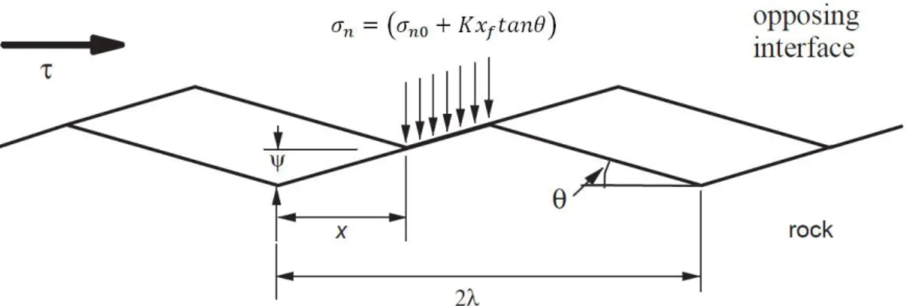
Seidel et Haberfield [2002] developed theoretical models to predict the shear behaviour of soft rock joints. Their model is composed of two independent mechanisms; initial sliding along the surface of the asperities and then simultaneous shearing through all of the intact asperities (Figure 1.13). The consequence of this sliding is joint dilation and stress localization on the steepest asperities in contact. The steepest asperities are sheared when the shear stresses exceed the asperities’ strength. Then the shear stresses are shed to the next-steepest asperities and these asperities control the dilation until they also fail in shearing.

According to Seidel et Haberfield [2002], the failure shear stress ( ) for the frictional asperity sliding model is given by:

_(1.13)

and for the failure of triangular asperity can hence be computed by:

( ) (1.14)

where is base friction angle of the joint, is asperities inclination, is initial normal

stress, K is stiffness and is shear displacement at failure.

Figure ‎1.13. Reduction of asperity contact area with progressive shear displacement and local normal

(36)

Grasselli et Egger [2003] introduced quantitative three-dimensional surface parameters into a shear strength criterion. It was based on detailed surface measurements of the joints, using an optical measurement system called ATOS (Advanced Topometric System). They stated that degradation is more likely to occur in steeper asperities. Therefore, instead of considering the whole contact area between surfaces, an effective contact area ( ) should be considered in the shearing process. They explained that effective contact areas only occur in asperities that are facing the shear direction. Moreover, they stated that only the steepest asperities (steeper than a threshold inclination, ) are in contact in the shearing process and are deformed,

sheared or crushed depending on the applied normal load.

To describe the relationship between the effective contact area ( ) and the corresponding minimum apparent dip angle (Figure 1.14) of asperities facing shear direction ( ); the following equation was adopted to fit the data:

(

) (1.15)

where A0 is the maximum possible contact area in the shear direction which usually is around 50% of the total potential area for fresh mated discontinuities. is the maximum apparent

dip angle in the shear direction, and C is a “roughness” parameter, calculated using a best-fit regression function, which characterizes the distribution of the apparent dip angles over the surface.

(37)

Figure ‎1.14. Geometrical identification of the apparent dip angle in function of the shear direction [Grasselli, 2001].

Based on his experimental results, Grasselli et Egger [2003] proposed the following empirical expression to predict the peak shear strength.

(1.16)

where is the applied average normal stress, is the residual friction angle (after a standard displacement of 5 mm), and g is a term which account for the contribution to peak shear strength from surface morphology given by:

(1.17)

where is the tensile strength of the intact rock material. The residual friction angle ( ) could be expressed as:

(38)

( ) (1.18)

where β is the contribution from roughness to the residual friction angle. The parameter α is the angle between the schistosity plane and the normal of the joint. If no schistosity planes are present α is set to zero.

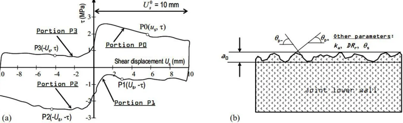
Belem et al., [2004] suggested a criterion to predict the peak shear strength ( ) under both constant normal load and constant normal stiffness. This criterion can take into account the anisotropy of surface morphology of irregular and regular joint surfaces:

[ ( ( ))]

[ ( ) ( ( ))] (1.19)

where is the initial normal stress, is basic friction angle, is the directional

dilatancy-degradation angle, is shearing direction angle, is degree of apparent anisotropy of surface morphology, is normal stiffness, is shear displacement for one cycle of shearing, is peak dilatancy angle (Figure 1.15).

Figure ‎1.15. Shear strength model parameters: (a) typical cyclic shear curve showing the four portions;

(b) morphological parameters [Belem et al., 2004].

The first terms of the Equation 1.19 correspond to the constant normal loading path and the second terms correspond to the constant normal stiffness loading contribution. When K = 0, equation predicts the directional peak shear stress of constant normal loading path and when

(39)

K > 0, equation predicts the peak shear stress of constant normal stiffness loading path. The dilatancy-degradation angle ( ) is given as follows:

( [

( )

]) _(1.20)

where is the mean angle of surface asperities or surface angularity parameter, is joint surface amplitude, is number of cycles of shearing (For monotonous shearing n = 1) and is the degree of joint surface relative roughness.

Based on asperity angles, Park et al., [2013] characterized the joint surfaces by introducing a concept named ‘micro-slope angle’ which is an extension of the ‘apparent dip angle’ suggested by Grasselli et Egger [2003]. By back-analyzing the shear and normal displacements obtained from laboratory shear tests and the micro-slope angle concept, Park et al., [2013] introduced a numerical method to determine the contact areas of a rock joint under normal and shear load. They showed that most of the contact areas occur in the regions facing the shear direction, and the asperities with flatter slopes were less likely to come into contact. Park et al., [2013] developed a model using an empirical approach basis on a new three dimensional quantitative roughness parameter to predict the shear behavior under CNS as well as CNL conditions. This parameter, the active roughness coefficient (Cr), was derived from the features of the effective roughness mobilized at the contact areas during shearing. They established the peak friction coefficient ( ) as:

( )

⁄ (1.21)

where A, B, C, and D are dimensionless parameters used to fit the experimental data.

In the model, four terms are used: the ratio of tensile strength to initial normal stress ( ⁄ ),

the active roughness coefficient (Cr), the friction coefficient mobilized by the basic friction angle ( ), and the ratio of normal stiffness to initial normal stress ( ⁄ ). The

(40)

applicability of the suggested model, while the last term has units of reciprocal length. If Cr is zero, Equation 1.21 represents the behavior of a planar joint; the peak friction coefficient is only attributed to the basic friction angle.

Park et al., [2013] calculated parameters A, B, C and D according to the results of multiple regression analysis using 362 experimental data. They presented the following equations 1.22 and 1.23 for CNS and CNL loading conditions respectively:

( ) ⁄ (1.22) ( ) (1.23)

1.2.2 The effect of loading conditions on shear behaviour of rock joints

The variety of field loading conditions is the main problem in studying the effect of field loads on the shear behaviour of discontinuities. Many of the field loads, which must be considered in the study of discontinuities’ behaviour, fall into three categories: monotonic, large-displacement (post-peak) cyclic loading and small-large-displacement (pre-peak) cyclic loading. Many researchers studied the shear behaviour of rock joints under monotonic loading conditions and proposed shear strength criteria to describe the variation of the peak shear strength under monotonic loading conditions [Patton, 1966; Ladany et Archambault, 1969; Barton, 1973; Gens et al., 1990; Amadei et Saeb, 1990; Grasselli et Egger, 2003; Roosta et al., 2006; Park et al., 2013]. Most of the constitutive models developed for monotonic loading conditions are not suitable for taking into account the effect of the cyclic loading conditions on predicting the shear behavior of rock joints [Belem et al., 2007; Nemcik et al., 2014].

Most of the initial research on the large-displacement (post-peak) cyclic loading tests was focused on determining the stress-displacement relationship and the peak shear strength of the cyclic loading tests. Jing et al. [1993], Souley et al. [1995], Fox et al. [1998], Jafari et al. [2003], and Nemcik et al. [2014] have proposed some models to predict the shear behavior of

(41)

rock joints and Crawford et Curran [1981], Curran et Carvalho [1983], Hutson et Dowding [1990], Barbero et al. [1996], Homand-Etienne et al. [1999], Jafari et al. [2003] have studied the shear strength of rock joints subjected to large-displacement (post-peak) cyclic loading conditions. These researchers reported that the shear strength is a function of joint roughness, number of cycles and, normal stress. Also, under low normal stress, the dynamic shear strength is greater than the corresponding static value and this effect decreases with increasing normal stresses.

After the initial efforts to explain the effects of large-displacement (after-peak) cyclic loading on predicting the peak shear strength and the shear behavior of rock joints, most of the research focused on studying the influence of the asperity degradation on the mechanical behaviour of rock joints under cyclic loading conditions. Also, recently, the effect of small-displacement (pre-peak) cyclic loading on the shear strength parameters of rock joints was studied by Jafari et al. [2003; 2004], Ferrero et al. [2010], and Tsubota et al. [2013]. For example:

Lee et al. [2001] indicated that the shear behavior of asperity under cyclic shear loading would be different according to the shear direction (forward or backward shearing), the type of asperities and the strength of rock materials. They prepared two types of joint by saw-cut (smooth joint) and split tensile (rough joint) method. They demonstrated that shear behavior of smooth joints is strongly affected by the surface friction and shear behavior of rough joints in first loading cycles is significantly affected by the degradation of the second order asperities (Figure 1.16). For the second and subsequent shear loading cycles, cyclic shear behavior is overwhelmingly affected by the first order asperities.

(42)

Figure ‎1.16. Cyclic shear behavior of smooth (top photo) and rough (bottom photo) joints [Lee et al., 2001].

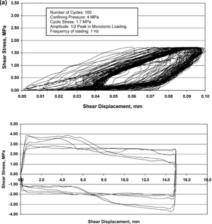
Jafari et al. [2003] also studied the influence of the cyclic shear tests on the degradation of an undulated artificial joint of mortar and found that during cyclic shear displacement, degradation will occur, depending on the cyclic displacement magnitude and normal stress applied. During small cyclic loading and low amplitude of cycles (Figure 1.17a), asperities will be slightly affected, but during large cyclic loading when amplitude of cycles are high (Figure 1.17b), asperities may be totally damaged.

Jafari et al. [2003] demonstrated that the shear strength of joint replicas is decreased under small cyclic loading conditions. The number of load cycles and stress amplitude are two main parameters controlling the shear behaviour of rock joints during cyclic loading. Dilation angle,

(43)

degradation of asperities and wearing are three main factors which affect the shear strength of rock joints during large cyclic loading conditions. The shear behaviour of rock joints during sliding is in direct relation to the level of normal stress.

Figure ‎1.17. Shear stress–shear displacement curve of small cyclic displacement and large cyclic

displacement [Jafari et al., 2003].

Based on the experimental results, Jafari et al. [2003] developed mathematical models to predict the shear strength of rock joints subjected to cyclic loading conditions. They proposed Equation 1.24 in the case of small-displacement cyclic loading (shear velocity from 0.05 to 0.4 mm/sec and maximum shear displacement of 0.1 mm):

(1.24)

where

is the number of stress cycles, is the normalized shear velocity, is the normalized stress amplitude, a = 0.3, m = -0.045, n = -0.17.

(44)

In the case of large-displacement cyclic loading (maximum shear displacement of 15 mm), the following relation was proposed:

(1.25)

where is the number of displacement cycles, in is the normalized dilation angle, Dn is the normalized degradation (normalized by maximum value of asperity amplitude), B = -0.33, c = 1.44, p = 0.12, q = 0.3.

Belem et al. [2007] conducted tests on three different specimens with different shapes (hammered, corrugated and rough) under monotonic and large-displacement cyclic loading conditions. They scanned the joint surfaces of specimens before and after each shear test using a laser scanner profilometer. Based on the experimental results and previously proposed surface roughness description parameters [Belem et al., 2004], they have proposed two experimental asperity degradation models to describe the evolution of initial surface roughness (first-order and second order roughness) during shearing under both constant normal stress (Equation 1.26) and constant normal stiffness (Equation 1.27) loading conditions:

( ) ( ) (1.26)

[ ( )] (1.27)

where is progressive degradation, is normal stiffness, is relative or shear

displacement, is the average dilation angle, is calibration factor (

) and is progressive degradation parameter that is a function of shear displacement (us) and surface morphology.

Ferrero et al. [2010] evaluated rock joint damage after small-displacement (pre-peak displacement controlled) cyclic loading tests. They carried out the cyclic tests on either smooth or rough discontinuities. They scanned the joint surfaces before and after each test and studied the surface damages using the damage mechanics model proposed by Belem et al. [2007]. They showed that progressive surface damage and, consequently, regressive shear strength are

(45)

related to the cyclic frequency, the normal stress, the roughness, the surface compressive strength and the number of cycles.

1.2.3 The effect of boundary conditions on shear behaviour of rock joints

Rock joints can be subject to different types of boundary conditions in the field ranging from constant normal load (CNL) to constant normal stiffness (CNS) and joint shear strength depends on those boundary conditions.

The constant normal load (CNL) mode of shearing is suitable for situations that dilation is permitted to occur freely or there is no dilation during the shearing process. Shear testing under a constant normal load (CNL) boundary condition may reproduce discontinuity behaviour in the case of sliding of a non-reinforced block of rock from a slope (Figure 18). For rough discontinuities that dilation may be inhibited by the surrounding rock, an increase in the normal stress occurs with shear displacement. Therefore, shearing of rough joints does not take place under constant normal load, but under variable normal load. This mode of shearing (CNS) is suitable representative of discontinuities isolated a block that may potentially slide or fall from the periphery of an underground excavation (Figure 18).

As Figure 19 shows, in general, the shear strength of a joint under constant normal stiffness (CNS) boundary conditions is higher than its shear strength under constant normal load (CNL).

(46)

Figure ‎1.18. Range of boundary conditions across a joint surface.

Figure ‎1.19. Shear stress vs. shear displacement models (a) Constant stiffness model, (b) Constant

(47)

1.3 Objectives

The main objective of the thesis is to study the changes of asperities’ role in three-dimensional with respect to their geometric parameters under various types of loading. This study will allow a better comprehension of the shear mechanism of rough surface and it will provide a detailed insight into the prediction of shear strength parameters of rock joints. This objective has been subcategorized as below:

 Characterizing the joints’ surface with a mathematical expression based on geometric dimensions of asperities. For this purpose, three-dimensional coordinates of joint surfaces are required. A procedure for moulding and scanning the joint surfaces before and after each test is proposed. Based on the joint surface characterization, the following investigations should be possible.

- Calculating asperities’ angles and roughness parameters for different directions. - Plotting the maps of topography and angles distribution.

 Developing a methodology for detecting contact areas and damaged areas at various shear displacements. Then, it is tried to link these areas to the geometric parameters of asperities. Classifying in-contact asperities according to their heights and angles at various shear displacements can explain the geometric effect of asperities on shear mechanism during different stages of shearing.

 Studying the changes of the roles of asperities under various types of loadings. These changes are studied with identifying in-contact asperities and investigating their reaction at different stages of shearing under monotonic and four types of pre-peak loading-unloading conditions.

More specifically, the finding of several experimental tests through this methodology will be helpful to provide a better explanation of the complex mechanism of shearing during pre-peak, peak, post-peak and residual stages.

(48)

1.4 Originality and Contribution

Three-dimensional tracking of changes of asperities is one of the most important ways to illustrate shear mechanism of rock joints during testing. Many studies that attempted to explain the asperities roles on rock joint shear behaviour were limited to consider the surface roughness along linear profiles [Patton, 1966; Barton et Choubey, 1977; Seidel et Haberfield, 2002] while joint surfaces are three-dimensional and quantification of surface roughness on three-dimensional space has higher accuracy. Some researchers, such as Gentier et Hopkins [1997], Lanaro et al. [1998], Gentier et al. [2000], Grasselli et Egger [2000], Homand et al. [2001], Xia et al. [2014], tried to link the three-dimensional surface roughness with shear strength. However, engineers and scientists are still looking to answer some questions that none of previous researchers attempted to explain.

 Which types of asperities according to their geometric properties contribute the most to shear mechanism in pre-peak, peak, post-peak and residual stages of shearing?

 Is there any change on asperities role under different loading conditions?  Is there the same role for all in-contact asperities during the shear process? The originality of this thesis can be categorized into the following sections:

 Previous researchers have not described the various contributions of steepest asperities that their faces are in shear direction on shear mechanism during a test. In this thesis a methodology was developed that can detect contact areas during shear tests then separate the role of those areas to just sliding or eroding and link them to their geometric properties. It can provide clear perspective of the sequence of asperities roles during shear test.

 Beside the joint characteristics, the loading conditions have significant effects on shear behaviour of rock joints. Previous researchers have mainly studied the three-dimensional asperities contribution of real joint surfaces under monotonic loading conditions. In this thesis, the three-dimensional asperities contribution of real joint surface is assessed, not only under monotonic loading, but also under various cyclic loadings. Through experimental results under monotonic and various cyclic loading,

(49)

this project seeks to generate more statistically robust and detailed data for loading effect on shear mechanism.

1.5 Thesis Outline

This thesis is comprised of three journal papers. Each paper is a chapter of the thesis which includes introduction and conclusion. In addition, Chapter 1 is the introduction of the thesis and literature review, and conclusions and perspectives are presented in Chapter 5.

Chapter 1 demonstrates problem statements, literature review, objectives of the research, originality of the thesis and thesis outline.

Chapter 2 illustrates a new methodology for characterizing joints’ asperities with a mathematical expression. At the beginning of this chapter a new algorithm for joints’ asperities characterization is presented. Then the performance of the proposed method is verified for predicting the distribution and size of the damaged areas in comparison with image analysis results. The properties of asperities that are in-contact during pre-peak, peak, post-peak and residual stages of shearing are identified. Also, the relation between in-contact asperities and their angles and heights at different shear displacements is discussed. The output of this chapter was submitted to ock Mechanics and ock Engineering journal. “Geometric effect of asperities on shear mechanism of rock joints” is proposed as the title for this paper. Chapter 3 is devoted to the influence of different number of pre-peak cyclic loading on shear behaviour of rock joints. The joint surface of specimens is characterized after scanning the joint surfaces before and after each test. Subsequently, after detecting contact and damaged areas the degradation of asperities during pre-peak stage of shearing and after various number of cycles is evaluated. Then the effect of various number of pre-peak cyclic loading on the peak shear strength and post-peak stage of shearing is explained. These results are compared with the results of monotonic tests to clarify the effect of pre-peak cyclic loading. The output of this chapter was submitted to International Journal of Rock Mechanics and Mining

(50)

Sciences. “Shear mechanism of rock joints under pre-peak cyclic loading conditions” is proposed as a title of this paper.

Chapter 4 presents the influence of various types of pre-peak cyclic loading on joint shear mechanism with attention to asperities degradation. Some replica specimens were cast using a joint surface of a granite block. Four different types of pre-peak cyclic loading as representatives of field loading conditions are applied on the joint replica specimens. Two monotonic shear tests were also run as the basis for comparison with the results of the cyclic loading tests to explain the effect of various pre-peak cycles of loading on the shear behaviour of specimens. The proposed method in Chapter 2 was used to characterize the specimens’ surfaces and track the changes of the role of in-contact asperities during pre-peak cyclic loading tests in order to provide a better explanation of their shear mechanism. The output of this chapter is submitted to Journal of Rock Mechanics and Geotechnical Engineering. “Shear mechanism of rock joints under various types of pre-peak loading-unloading conditions” is proposed as a title of this paper.

Conclusions and recommendation for subsequent studies are provided in the last chapter of the thesis (Chapter 5).

(51)

29

CHAPTER 2. GEOMETRIC

EFFECT

OF

ASPERITIES ON SHEAR MECHANISM OF

ROCK JOINTS

2.1 Avant-propos

Auteurs et affiliation :

 Ali Fathi: Étudiant de doctorat, Université de Sherbrooke, Faculté de génie, Département de génie civil.

 Zabihallah Moradian: Postdoctoral associate, Department of Civil and Environmental Engineering and Earth Resources Lab (ERL), Massachusetts Institute of Technology (MIT), Cambridge, MA, USA.

 Patrice Rivard: Professeur titulaire, Université de Sherbrooke, Faculté de génie, Département de génie civil.

 Gerard Ballivy: Professeur adjoint, Université de Sherbrooke, Faculté de génie, Département de génie civil.

 Andrew J. Boyd: Professeur, McGill University, Department of Civil Engineering. État : Accepte

Date de présentation: 7 october 2014

Revue : Rock Mechanics and Rock Engineering Référence : [RMRE-D-14-00535R3]

Titre français: Effet de la géométrie des aspérités sur le mécanisme de cisaillement des joints

- rocheux

(52)

Contribution

The quantifying three dimensional surfaces characteristics, detecting in-contact asperities during shear test and describing them according to their geometric dimensions is one of the main objectives of this thesis. To accomplish this requires a new methodology for characterizing joints’ asperities with a mathematical expression is illustrated in this chapter. Also, the geometric characterization of the effective (in-contact and damaged) areas in the shearing process under different levels of normal stress and during different stages of monotonic shearing is studied.

The influence of various types and numbers of cyclic loading in the asperities degradations is studied in Chapters 3 and 4. The geometric effect of asperities on shear mechanism of rock joints under cyclic loading is also studied.

Abstract

Three-dimensional tracking of changes of asperities is one of the most important ways to illustrate shear mechanism of rock joints during testing. In this paper, the changes of the role of asperities during different stages of shearing are described by using a new methodology for the characterization of the asperities. The basis of the proposed method is the examination of the three-dimensional roughness of joint surfaces scanned before and after shear testing. By defining a concept named ‘tiny window’, the geometric model of the joint surfaces is reconstructed. Tiny windows are expressed as a function of the x and y coordinates, the height (z coordinate), and the angle of a small area of the surface. Constant normal load (CNL) direct shear tests were conducted on replica joints and by using the proposed method, the distribution and size of contact and damaged areas were identified. Image analysis of the surfaces was used to verify the results of the proposed method. The results indicated that the proposed method is suitable for determining the size and distribution of the contact and damaged areas at any shearing stage. The geometric properties of the tiny windows in the pre-peak, peak, post-peak softening and residual shearing stages were investigated based on their angle and height. It was found that tiny windows that are facing the shear direction, especially the steepest ones, have the primary role in shearing. However, due to degradation of asperities at higher normal

(53)

stresses and shear displacements, some of the tiny windows that are not initially facing the shear direction also come in contact. It was also observed that tiny windows with different heights participate in the shearing process, not just the highest ones. Total contact area of the joint surfaces was considered as summation of just in-contact areas and damaged areas. The results of the proposed method indicated that considering differences between just in-contact areas and damaged areas provide useful insights into understanding the shear mechanism of rock joints.

2.1 Introduction

Understanding the shear mechanism of rock joints is a key step for designing geotechnical projects that include discontinuities. The shear mechanism of joints is strongly affected by the joint roughness, the loading conditions, and the mechanical properties of the rock [Barton, 1973; Kulatilake et al., 1995; Re et Scavia, 1999; Gentier et al., 2000; Yang et al., 2001; Lopez et al., 2003). The shear mechanism of rock joints is the basis of constitutive models for predicting the shear strength of rock joints. One of the early researchers who considered shear mechanism of asperities in the description of shear strength was Patton [1966]. He studied the shear behaviour of “saw-tooth” joints. Patton observed that sliding occurred along the intact asperity when the effective normal stresses were low and the effect of the intact asperities disappeared due to the shearing of the asperity when effective normal stresses were high. He proposed the following bilinear failure criterion:

(for low effective normal stresses) (2.1) (for high effective normal stresses) (2.2)

where is the peak shear strength, is the normal stress, is the basic friction angle, is the residual friction angle, is the cohesion when the asperities are sheared, and i is the angle of the “saw-tooth” asperities with respect to the shear direction. According to Ladanyi et