Counting processes and copulas : applications in insurance

COUNTING PROCESSES AND COPULAS: APPLICATIONS IN IN-SURANCE

DISSERTATION PRESENTED

AS PARTIAL REQUIREMENT TO THE MASTER IN MATHEMATICS

BY

FRANK BARNING

Avertissement

La diffusion de ce mémoire se fait dans le respect des droits de son auteur, qui a signé le formulaire Autorisation de reproduire et de diffuser un travail de recherche de cycles supérieurs (SDU-522 - Rév.10-2015). Cette autorisation stipule que «conformément à l'article 11 du Règlement no 8 des études de cycles supérieurs, [l'auteur] concède à l'Université du Québec à Montréal une licence non exclusive d'utilisation et de publication de la totalité ou d'une partie importante de [son] travail de recherche pour des fins pédagogiques et non commerciales. Plus précisément, [l'auteur] autorise l'Université du Québec à Montréal à reproduire, diffuser, prêter, distribuer ou vendre des copies de [son] travail de recherche à des fins non commerciales sur quelque support que ce soit, y compris l'Internet. Cette licence et cette autorisation n'entraînent pas une renonciation de [la] part [de l'auteur] à [ses] droits moraux ni à [ses] droits de propriété intellectuelle. Sauf entente contraire, [l'auteur] conserve la liberté de diffuser et de commercialiser ou non ce travail dont [il] possède un exemplaire.»

PROCESSUS DE COMPTAGE ET COPULES: APPLICATIONS EN ASSURANCE

MÉMOIRE PRÉSENTÉ

COMME EXIGENCE PARTIELLE DE LA MAÎTRISE EN MATHÉMATIQUES

PAR

FRANK BARNING

Tout d'abord, je remercie Dieu Tout Puissant d'avoir veillé sur moi durant toutes ces années d'étude. Ensuite, j'exprime mon admiration et profonde gratitude à mes surper-viseurs, Dr. Matthieu Dufour et Dr. Michel Adès. Je leur dois beaucoup pour tout le support, l'inspiration, les conseils et surtout leur engagement à l'excellence. Ils ont été essentiels, non seulement, pour le succès de ce travail mais aussi pour mon progrès et bien-être. Je suis égalementreconnaissant à tous les membres du département de math-ématiques de l'UQAM pour ce magnifique environnement propice à notre étude. J'ai apprécié tous les conseils, l'enseignement et les services inestimables que vous m'avez donnés afin d'assurer un environnement d'étude confortable et épanouissant.

Je remercie de façon particulière Mme Gisèle Legault, analyste au département de mathématiques pour sa disponibilité et son expertise informatique bien utile et forte-ment appréciée.

Je remercie ma chère épouse Naomi Armah, ma chère fille Elliette N. Barning, ma mère Gladys Dansowaa et mon frère Chris Arthur. Vous êtes toutes et tous très chers à mon cœur.

LIST OF TABLES . LIST OF FIGURES LIST OF SYMBOLS RÉSUMÉ . . ABSTRACT INTRODUCTION CHAPTER I

MODELLING DEPENDENCE WITH COPULAS 1.1 Overview of Modelling Dependence

1.2 What are copulas? . . . .

vii . viii ix X xi 1 4 4 5 1.2.1 Historical Background on the Development of Copula Theory 5

1.2.2 Why Do We Care About Copulas? . 6

1.3 Multivariate Copulas . . . .

1.4 Fundamental Computational Techniques U sed In Copula Theory 1.4.1 The Fréchet-Hoeffding Bounds . . . . 1.4.2 Switching from Distribution to Survival Functions 1.4.3 Invariance Under Strictly Monotone Transformations . . 1.4.4 Copula Derivatives . . . . 1.5 How to Measure Dependence Structure In Copula Theory .

9 10 10 11 13 14 15 1.5 .1 Classical Linear Correlation . . . 15 . 1.5 .2 Measures of Concordance And Expressing them as a Function of

Copulas . . . 16

1.5 .3 Examples of Measure of Concordance . . 18

1.6.1 Implicit Copulas 1.6.2 Explicit Copulas 1. 7 Counting Processes . . .

1. 7 .1 Application of Compound Processes in Insurance . 1.8 Organization for the rest of this Research Work . . . . CHAPTER II

REVIEW OF DIFFERENT COPULAS RELATING TO COUNTING PROCESSES 20 21 22 25 27 IN INSURANCE TOPICS . . . ~ . . . 30 2.1 Copula-Based Dependence Between Frequency and Class in Car

In-surance with Excess Zeros 30

2: 1.1 Introduction . . . . . 2.1.2 Model Specification 2.1.3 Parameter Estimation .

2.1.4 Algorithm for Implementation 2.1.5 Summary and Discussion . . .

2.2 A Mixed Copula Model for Insurance Claims and Claim Sizes 2.2.1 Introduction . . . . . 2.2.2 Model Specification 2.2.3 Parameter Estimation . 30 31 35 37 38 39 39 40 44 2.2.4 Algorithm for Implementation: Poisson-Gamma Regression Model 50 2.2.5 Summary and Discussion . . . 51 2.3 Moments of the Aggregate Discounted Claims with Dependence

lntro-duced by a FGM Copula 53

2.3 .1 Introduction . . . . 2.3 .2 Model Specification 2.3.3 Summary and Conclusion

53 53 64 2.4 Modelling Dependence in Insurance Claims Processes with Lévy Copulas 66 2.4.1 Introduction . . . 66

2.4.2 Existing Approaches in Modeling Dependence in Multiple Com-pound Poisson Processes . . . 67 2.4.3 Dependence Modeling of Multiple Compound Poisson Processes

withLévy Copulas . . . 68

2.4.4 Lévy Copulas and Compound Poisson Process 70

2.4.5 How Lévy Copulas are Built. . . 73 2.4.6 Comparing Dependence Structures among two (2) Lévy Copulas

(LCl-2) under the current context 74

2.4.7 Parameter Estimation . . . 77 2.4.8 Maximizing the Likelihood Function by the Method of Inference

Functions for Margins (IFM) . . 80

2.4.9 Algorithm for Implementation 80

2.4.10 Summary and Discussion . . .

2.5 Multivariate Counting Processes: Copula and Beyond . 2.5 .1 Introduction . . . .

2.5.2 Model Specification

2.5.3 Dependence in Thinning and Shift (TaS) Models 2.5.4 Conclusion

CHAPTER III

DATA, METHODOLOGY AND ESTIMATION 3.1 Overview

3.2 Data . . . . 3.3 Methodology

3 .4 Inference - Estimation and Asymptotic Property . . 3.4.1 Maximum Likelihood Estimation

3.4.2 The Profile Likelihood CHAPTER IV

ANALYSIS, DISCUSSION AND CONCLUSION 4.1 Analysis of Results . . . .

...

82 83 83 84 89 94 95 95 95 96 98 98 99 . . 101 .. 101

4.2 Discussion . . 4.3 Conclusion APPENDIX A RESULTS . . . . APPENDIX B

SOME FEATURES OF THE COPULAS USED IN THIS MATERIAL B.1 Farlie-Gumbel-Morgenstem (F-G-M) Copula

B .1.1 Formula for Distribution Function B.1.2 Formula for Density Function B.1.3 Correlation Coefficient B.1.4 Dependence Properties B .2 Clayton Copula . . . .

B .2.1 Formula for Distribution Function B .2.2 Formula for Density Function B.2.3 Kendall's Tau . . . . B.2.4 Low-Tail Dependence (LT). B.2.5 Truncation-Invariance Property APPENDIX C

RCODE . . . .

C.1 R Code to implement algorithm in Section 2.1 . . BIBLIOGRAPHY . . . . . . 105 . . 106 . 108 . . 113 . . 113 . 113 . . 113 . . 113 . . 114 . 114 . . 114 . . 114 . 114 . . 114 . . . 114 . 115 . . 115 . . . . 118

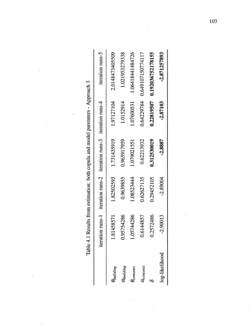
Table Page 2.1 Illustration from the example: Source Bauerle and Grübel (2005) 92 4.1 Results from estimation: both copula and model paremters - Approach

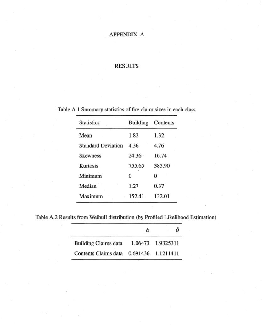
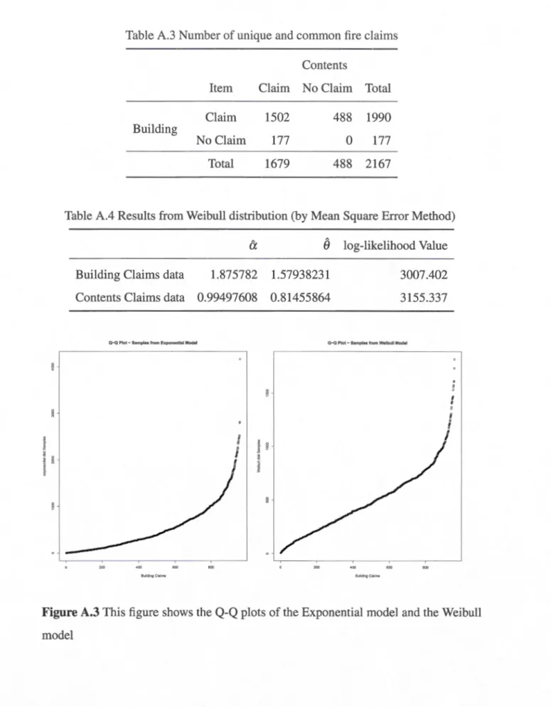
3 . . . . 103 A.1 Summary statistics of tire claim sizes in each class . . 108 A.2 Results from Weibull distribution (by Profiled Likelihood Estimation) . 108 A.3 Number of unique and common tire daims

. . .

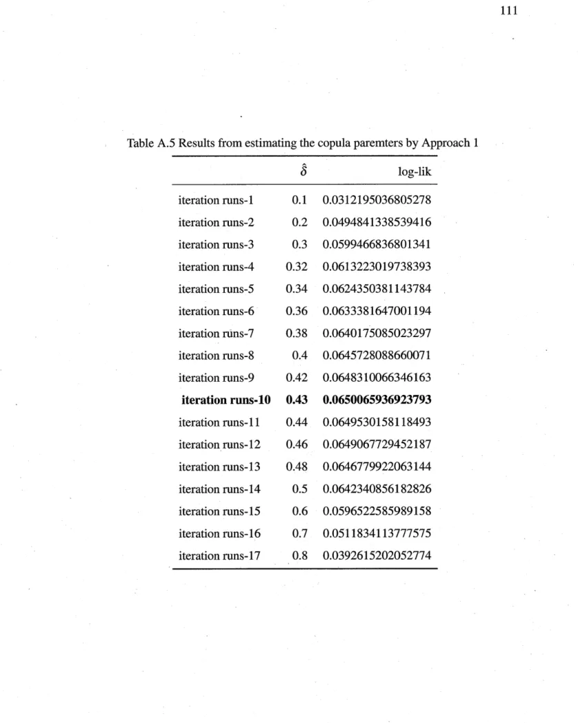
. . 110 A.4 Results from Weibull distribution (by Mean Square Error Method) . . 110 A.5 Results from estimating the copula paremters by Approach 1 . 111 A.6 Results from estimation: copula paremters by Approach 2

..

.. 112

Figure Page 1.1 This figure shows how Chapter 1 and Chapter 2 of this thesis is organized 28 1.2 This figure provides a further description to the earlier figure

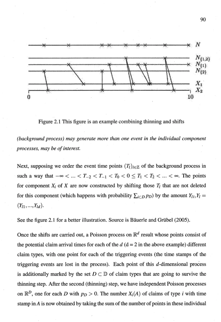
2.1 This figure is an example combining thinning and shifts . . .

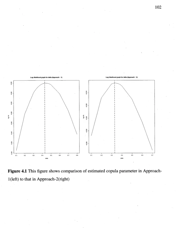
4.1 This figure shows comparison of estimated copula parameter in Approach-29 90

1 (left) to that in Approach-2(right) . . . 102 A.1 This figure shows a cumulative distribution fit of Weibull model (red)

and Exponential model (blue) . . . 109 A.2 This figure shows profile likelihood estimation for Weibull model

pa-rameters for Building random variable . . . 109 A.3 This figure shows the

Q-Q

plots of the Exponential model and the

J_

Il

MBP · IBNR MLE iid

Ps

'! CPP U[O,

1]

GLM IFM LCl

ë

lA(x)

F,G,Fï, etc. F=l-F pdf C

(.Q,$,JP)

R,R+

Pc

U(a,b)

unique corn.mon Maximization by Parts

lhcurred But Not Reported Claims Maximum Likelihood Estimation independent and identically distributed Spearman's· Rho

Kendall' s Tau

Compound Poisson Processes

Uniform distribution on the interval

[O, 1]

Generalized Linear Regression Models Inference Functions for Margins

Lévy Copula 1, as a notation for a type of Lévy Copula Survival copula

indicator fonction (of a set A):

lA(x)

=

1 if

x

E A and otherwise 0 cumulative distribution fonctions ( cdf)

univariate survival fonction "probability density fonction" copula

probability space

real line, non-negative real line

probability measure induced by a copula C uniform distribution on ( a, b)

Les processus de comptage ont un rôle majeur et des applications variées dans plusieurs domaines telles que la tarification, la réserve de perte, l'allocation du capital en assur-ance. Avec toutes ces applications, il y a quelques risques ou des facteurs de risque qui dépendent sur un autre ensemble de risque ou des facteurs de risques, et cela con~ stitue précisément un grand intérêt pour les compagnies d'assurance. Ces compag-nies d'assurance veulent construire des modèles spécifiques pour capturer quelques, ou toutes les, structures de dépendance existantes entre 1es risques connus. Quelques-uns de ces risques connus sont associés avec les processus de comptage. La modélisation de la dépendance utilisant la théorie des copules et les processus de comptage a attiré l'attention de plusieurs chercheurs ces dernières années. Dans ce mémoire, nous étu-dions deux champs d'intérêt dans la modélisation de la dépendance avec applications en assurance et finance. Premièrement, nous étudions plusieurs méthodes de modélisa-tion, les techniques d'estimation et l'implémentation des algorithmes qui sont utilisés dans la modélisation des copules autour des· processus de comptage. Par exemple, dans le deuxième chapitre deux de ce mémoire, nous allons étudier comment la modélisa-tion de la dépendance est utilisée pour un risque bivarié ou pour des facteurs de risque telle que la classe Bonus-Malus et les comptes de réclamations du passé, le compte de réclamations et.la taille des réclamations, le compte de réclamations de deux processus de comptage différents qui se sont produits à partir du même événement,etc. Dans la deuxième partie du mémoire, nous scrutons et adressons quelques remarques autour du choix de quelques copules de la première partie 1 de ce mémoire, et nous présentons une discussion au sujet des approches utilisées. Cette deuxième partie du mémoire est motivée par le fait que différentes analyses vont choisir un ensemble différent de distri-bµtions univariées pour ajuster les mêmes données et choisir différents types de copules pour modéliser les structures de dépendance. En fait, on cherche dans la secpnde par-tie à répondre à la question : Devons-nous dépendre sur les marginales même si nous avons un ensemble large de données disponibles ? En dernier lieu; nous discutons à propos des estimés des vrais paramètres de copule et nous analysons un ensemble de vraies données.

Mots-Clés : Processus de comptage, copule, structure de dépendance, paramètres de modèle, estimation, copule de Clayton, distribution conjointe, processus de Lévy.

Counting process has a major and several applications in different areas such as rate-making, loss reserving and capital allocation in insurance. Within all these applications, some risks or risk factors depend on the other set of risk or risk factors and this depen-dence is ofhigh interest to insurance companies, particularly rate-making actuaries and loss reserving actuaries. These insurance companies would want to build specific mod-els that captures some or all the dependence structures existing between· the known risks. Sorne of these known risks are associated with counting process. Modeling de-pendence using copula has drawn the attention of several authors in recent years. In this thesis, we study two areas of interest in dependence modeling with application in insurance and finance. First we study several modeling methods, estimation techniques and implemented algorithms that are used in copula modeling surrounding counting process. For instance, in chapter two of this thesis, we will study how dependence modeling is carried for bivariate risk or risk factors such current Bonus-Malus class and past count of claims, count of claims and size of claims, count of claims of two different counting processes that occurred from the same event etc. In the second part of the thesis, we investigate and address some concerns surrounding the choice of some the copulas in the first part of the thesis and present a discussion to the approaches that were used. This second part of the thesis is motivated by the fact that different analysts will select different set of univariate distributions to fit the same data and choose from different types of copula to model the dependence structures. In fact, the second part seeks to answer the question: Should we depend on the fitting of marginals even if we have large set of data available?. Lastly we discuss about the estimates of a true copula parameter as we analyze a real dataset.

keyworkds: Counting process, Copula, dependence structure, model parameters, es-timation, Clayton copula, joint distribution, Lévy process.

Two events A and B are dependent if the occurrence of one event changes the proba-bility of the occurrence of other event. For example, large values of event A always occur with large values of event B or large values of event A always brings about small values of event B. Linear dependence between two events is by far the most popular form of dependence in many disciplines especially in the financial community. lt is mostly measured with linear correlation coefficient (see chapter 1). Lawless (2014), in his article explained that, this linear correlation coefficient measures how close a point cloud is to a straight line.

Though the linear correlation coefp.cient, among many dependence measures, for exam-ple Kendall's Tau and Spearman's Rho, is by far the most popular dependence measure used, it is also often misunderstood as a general measure of dependence. The popu-larity of this linear correlation coefficient started with the ease with which it can be calculated and it is a natural scalar measure of dependence in elliptical distributions (i.e. probability distributions that generalize the multivariate normal distribution there by forming an ellipse, for example the multivariate t-distribution).

However, most random variables are not jointly elliptically distributed, and using linear correlation as a measure of dependence in such situations might prove very misleading (Erilbrechts et al., 2001). This motivated the use of concordance measures (see chapter 1 ). Two random variables are co°:cordant when large values of ·one go with large values of the other. The most obvious application of the concordance is to use them to measure the strength of dependence empirically observed in some set of data.

has become a major and flourishing topic: Even in traditional risk theory, individual risks have usually been assumed to be independent, this assumption is very convenient for tractability but it is not generally realistic. Think for example of the aggregate claim amount in which any random variable represents the individual claim size of an insurer's risk portfolio. When the risk is represented by residential dwellings exposed to danger of an earthquake in a given location or by adjoining buildings in fire insurance, it is unrealistic to state that individual risks are not correlated, because they are subject to the same event cause (Campana & Ferretti, 2005). Many more research work in actuarial science among others may be found in Frees et al. (1996), Free and Valdez (1998) and Frees and Wang (2005).

With the proliferation of large datasets from a variety of sources, perhaps the most pressing and ubiquitous challenge is posed by the need to "leverage/influence big data." This calls for ways to build dependence models involving hundreds, and even thousands of variables (Lawless, 2014).

Unfortunately the traditional measures of dependence: the linear correlation coefficient among others such as Kendall' s Tau and the Spearman' s correlation coefficient, just by themselves cornes with some amount of limitations for bivariate distributions. An interesting concept that makes it possible to study dependence in broader terms was proposed by the American mathematician Abe Sklar in response to a question posed by his French colleague Maurice Fréchet is Copula. Copulas are useful tool to model de-pendent data as they allow to separate the dependence properties of the data from their marginal properties and to construct multivariate models with marginal distributions of arbitrary form (Aristidis K. Nikoloulopoulos, Dimitris Karlis, 2007). For instance, in finance, copula is used in modelling dependence structures in the analysis of credit risks, the insolvency of several debtors at the same time or for insurances the risk of appearance of different daims at the same time have to be modeled to insure solvency of the bank and insurance, respectively, all the time. Modeling dependence between

asset retums and modelling the dependence between coinpanies default times are the most common financial modeling tasks for which copulas are applied frequently (Mai & Scherer, 2014).

Count data occur in several areas in actuarial studies. In property insurance models, insurance daims count form a core part of risk theory. Also in health insurance, count data models have been widely used to estimate the predictors of health care demand. · Many studies on copula published has revealed some dependence structures that exist between these count variables and other known variables in the insurance and finance setting. In recent times, modeling in insurance is moving towards a broader perspective on assets and liabilities where dependencies between proeesses (for example different lines of business, count of daims from an insurance company and its main reinsurer, IBNR problem where late daims arise from the same event, and the distribution of the next daim arrival) are taken into account.

The objective of my present work is to review some of the copulas used in models in the insurance and finance setting in order to explore some methods in constructing copulas, different estimation procedures and techniques used to select the best copula ( as this task is no very easy in practice ). This will encourage more of the copulas being applied and stimulate further developments of copulas in this area.

MODELLING DEPENDENCE WITH COPULAS

1.1 Overview of Modelling Dependence

Suppose there are d variables Yl, ···,Yd and the data set consists ofyi

=

(yn,

···,Yid) for i

= 1, ... ,

n considered as a random sample of size n; that is, the Yi are independent and identically distributed (i.i.d.) realizations of a random vector Y

=

(Y1, ... , Yd). For example, we can consider the data matrix Y given by:

Y11 Y12 YB Yld Y21 Y22 Y23 Y2d

Ynl Yn2 Yn3 Ynd

Two goals are interesting here. First is to study the probabilistic behaviour of each of one of thè component of Y and second, is to investigate the relationship between them. Similarly, in dependence modelling, the steps are:

(i) univariate models for each of the variables Y1, ... , Yd; (ii) copula models for the dependence of the d variables.

In step (i), the choices for univariate parametric familles with two or more parameters depends on the modality, tail-weight, scale of dispersion and asymmetry. After the univariate models are chosen, next in step (ii) copula models must then be considered

to model the dependence. 1.2 What are copulas?

Informally, copulas are fonctions that join or "couple" multivariate distribution fonc-tions to their one-dimensional marginal distribution foncfonc-tions (Nelsen, 1999). The pur-pose of a copulais to "glue together the margins" or "couple the individual probabil-ities" (hence the Latin term "copulare") in order to generate dependence between the variables (Genest & Neslehova, 2005).

1.2.1 Historical Background on the Development of Copula Theory

The history of copulas may be said to begin with (Fréchet, 1951). Fréchet's problem: given the distribution fonctions Fj

(j

=

1, 2, ... , d) of d random variables X1, X2, ... , Xd defined on the same probability space (.O.,!F,IID), whatcan be said about the setr(F1,F2, ... ,Fd) of d-dimensional distribution fonctions whose marginals are the given Fj? He added that, if the random variables X1 ,X2, ... ,Xd are independent then

is a member of the set r( F1, F2, ... , Fd). However the problem is what then are the other members of this set?

In 1959, Abe Sklar obtained the most important result in this respect, by introducing the notion, and the name, of a copula, and proving the theorem that now bears his name (Durante & Sempi, 2010).

In a more simplest possible terms, let us consider the Maurice Fréchet's problem by this way. Suppose that X and Y are two fire daim amounts, say, for which we know how to compute the probabilities IID(X

:S

x)

and IID(Y

:S

y) for any values x and y. Viewed as

fonctions of x and y, the probabilities F(x)

=

IP'(X ~ x) and G(y)

=

IP'(Y ~ y) are called the marginal distribution fonctions, or margins of X and Y . The question is then how to construct a model for the probability of the events { X ~ x} and {Y ~ y} occurring simultaneously, denoted IP'(X ~ x and Y ~

y),

while ensuring that X has distribution F and Y has distribution G. Sklar (1959) suggested the equation below as an idea to answer the problem:

IP'(X ~ x and Y~ y)= C{IP'(X ~ x),IP'(Y ~ y)} (1.1) where C is a specific fonction of two variables called a copula. From the above equa-tion, one can say that copulas are expressed in the form;

C{u, v}

=

IP'(U ~ u and V~ v). (1.2)

1.2.2 Why Do We Care About Copulas?

Copulas have been of interest to statisticians for two main reasons: firstly, as a way of studying scale-free measures of dependence; and secondly, as a starting point for con-structing families of bivariate distributions, sometimes with a vew to simulation (Fisher, 1997). In other words, we care about copulas because, copulas reveal the true nature of dependence between variables and lead to flexible multivariate models (Genest, 2011).

Example ).2.1

(Thefollowing example explains the intuition behind Sklar's work in afinancial setting (credit to (Cherubini et al., 2004)).

Assume a product written on the Nikkei 225 and S&P 500 indexes which pays, at some exercise date T, one unit if both are lower than some given levels KNKY and Ksp. The price of this digital put option is:

Where Q(KNKY, Ksp) is the joint risk-neutral probability that both the Japanese and US market indexes are below the corresponding strike prices. Also, r is the discounting rate and t is the time we at which we are pricing the option. A put option gives the holder an option to sell the underlying as set at a strike price K

if

the price of the underlying asset at the time of expiration is lower than K. How can someone going to buy a put option recover a price that are consistent with the market price or in order words, how can a put option buyer pay for a price which he or she will end up exercising the option at time of expiration?

In modelling, our first goal will be to study the probabilistic behaviour of each of the marginais and next we investigate their relationship. So we will need some models for the risk-neutral probability <CmKY that the Japanese Nikkei Index at time T will be below the level KNKY and also the risk-neutral probability Qsp that the US S&P Index at time T will be below the level Ksp. In financial terms, we are asking what is the forward price of univariate digital options with strike prices KNKY and Ksp; in statistical terms, we are estimating from the market data, the marginal risk-neutral distributions of Nikkei and S&P indexes. So our price can be written as;

where C( ·, ·) is a bivariate function and has a basic requirement to be in the unit in- · terval in order to be able to represent a joint probability distribution. Other three requirements also cornes into mind. First,

if

one of the two events has zero probability, the joint probability that both events occur must also be zero and Secondly,

if

one event will occur for sure, ·the joint probability that both the events will take place is the same as the probability that the second event will be observed. Lastly,

if

the probabilities of both the events increase, then the joint probability should also increase.

Below are some associated definitions and theorems. H-Volume is a volume contained by a rectangle

[x1

,x2] x

[y1

,Y2] of a 3 -dimensional fonction.

Definition 1.2.1 (2-Increasing)

Let 0-:/= S1,S2 CR= extended real line on {-oo,+oo} and let H be a S1 x S2-+ R fonction. TheH-volume of B= [x1,x2]

x [y1,Y2]

isdefinedtobe:

H is 2- increasing function if VH(B)

2::

0 for all B C S1 x S2. Definition 1.2.2 (Grounded)

Suppose b1 = maxS 1 and b2 = maxS2 exist. Then the margins F and G of H are given by

F : S1-+ R, F(x)

=

H(x,b2), G : S2-+ R,

G(y)

=

H(b1,y).

Suppose also a1

=

minS1 and a2

=

minS2 exist, then His called grounded if:

H(a1,Y) =H(x,a2)

=

0, forall (x,y) E S1

x S2

Definition 1.2.3 (Bivariate Copula)

A bivariate copula function is a function

C,

whose domain is

[O,

1 ]2

and whose range is

[O, 1]

with the following properties:

(BCJ): C(x)

=

Ofor all x E [O, 1]2 when at least one element of xis O; (BC2): C(x, 1)

=

C(l,x)

=

xfor all x E [O,

1)2;

(BC3): forall (a1,a2), (b1,b2) E

[O,

1]2

with a1:::; a2 and b1:::; b2, we have : Vc([a,b])

=

C(a2,b2)-C(a1,b2)-C(a2,b1) +C(a1,b1)

2::

O.

Where (BCl) denotes Bivariate Copula or Axiom or property 1. The fonction Ve is called the C- volume of the rectangle [a, b] x [c, d].

Theorem 1 (Sklar's Theorem)

Let H be a bivariate distribution function with marginal distributions F and G. Then there exists a copula C such that:

H(x,y)

=

C(F(x),G(y)) (1.4)

Conversely, for any distribution functions F and G and any copula C, the function H defined above is bivariate distribution function with marginal distributions F and G.Furthermore, if F and G are continuous, then C is unique.

Example 1.2.2

Consider thefunction n(u,

v)

=

uv. Thisfunction satisfies conditions (BCl), (BC2) and (BC3), and hence thefunction n(u,

v)

is a copula.

1.3 Multivariate Copulas

Inference for multivariate models and in particular higher dimensional copulas is a far less developed area of statistics than univariate applications. One reason for this is, that the likelihood usually is less tractable (Schepsmeier

&

Stober, 2014).

This section presents a brief extension of the bivariate copula theory. A multivariate copula can be used to specify a multivariate distribution and every multivariate distri-bution provides a multivariate copula. We extend the basic properties of the bivariate copulas to the multivariate case.

Definition 1.3.1 (Multivariate Copula)

A p-dimensional copula is a function C :

[O, 1

]P

---+

[O, 1]

that satisfies:

(MCI): C(u1, ... , Ui-1, 0, Uï+1, ... , up)

=

Ofor all

1:::;

i:::; p,

(MC3): Forai

:s;

b;,a;,bï E [O, 1],i

=

1, ... ,p,

2 2

L ... L

(-l)ii+ ... +iPC(u1,i1, ... ,up,ip)

2::

0

i1 =1 ip=l

where Uj,1

=

aj and Uj,2

=

bjfor j

=

l, ... ,p.

Theorem 2 (Sklar's Theorem - Multivariate Copulas)

Let H be a p-dimensional distribution fanction with margins F1, ... , Fp. Then there ex-ists a p-copula C such that for all x;· E IR,

H(x1, ... ,xp) .. C(F(x1), ... ,F(xp)) (1.5)

If F1, ... , Fp are continuo us, then C is unique.

Conversely, if Fi, ... ,Pp are distributionfanctions and C is a copula, then H defined by

1.5, is a joint distribution fanction with margins F1, ... , Fp.

1.4 Fundamental Computational Techniques U sed In Copula Theory

1.4.1 The Fréchet-Hoeffding Bounds

This is the original work of Hoeffding (1994) and Fréchet (1951) . Similar to the correlation coefficient and other. numeric dependence measures, there exist lower and upper bounds for ail copulas. This computational technique is mostly relevant when one is studying the most extreme negative and positive dependence within a family of copulas.

Theorem 3 (Fréchet-Hoeffding Bounds)

Let C be a copula. Then for every ( u,

v)

in [O, 1

]2,

Pro of. Let ( u,

v)

be an arbitrary point in [ 0, 1

]2.

Sin ce: C(u,

v)

<

C(u,

1)

=

u C(u,

v)

<

C(l,

v)

=

v

*

C(u,

v)

<

min(u,

v)

Furthermore from (BC3) in Definition 1.2.3;

Vc([a,b])

=

C(a2,b2)-C(a1,b2)-C(a2,b1)+C(a1,b1)

2 0

Vc([u, 1]

x [v,

1])

=

1-u-v+C(u,v)

2

0 C(u, v)

2

u+v-1

*

C(u,v)

2

max(u+v-1,0)

Theorem 4 (Multivariate Copula - Bounds) For every copula C and any u in

[O, l]P,

D

In the multidimensional case of the Fréchet-Hoeffding bounds, the upper bound is still a copula but the lower bound is not.

1.4.2 Switching from Distribution to Survival Functions

In some applications, for example in the context of portfolio credit-risk modelling, it is very natural to consider survival fonctions rather than distribution fonctions. For instance the lifetime of a company is a random variable X taking only positive values. Modelling with exponential distribution ( the most popular distribution on the positive half-axis), we have its probability distribution fonction as: f(x)

=

Âe-h. The above distribution bas many nice and useful analytical properties such as: F(x)

=

e-Àx and

F(x)F(y)

=

F(x+y), where F(x) is the survival fonction of x. Multivariate concepts of the exponential distribution rel y on a treatment of multivariate survival fonctions. In order to apply copula theory for these concepts, thesurvival analog of Sklar's Theorem is necessary.

Theorem 5 (Sklar's Theo:rem for Survival Functions)

AfunctionF(x): Rd--+

[O, 1]

is the survivalfunction of some random vector

(X1,X2, ...

,Xd)

if

and only

if

there are, a copulas

ê :

[O,

1 ]d --+

[O, 1]

and univariate functions F 1, ... , F d : R--+

[O, 1]

such that

The correspondence between F and

ê

is one-to-one if all survival fonctions F 1, ... ,_F d are continuous.

Example 1.4.1

Assume that

(X1,X2)

is a random vector on a probability space

(.Q,JF,P)

with dis-tribution function F(x1 ,x2) :=

1P(X1 ::; x1 ,X2 ::;

x2), which admits the representation F(x1 ,x2)

=

C(F1 (x1),F2(x2)

),for

x1

,x2

E

IR,

with a bivariate copula

C

and two univari-ate distribution functions

F1,

F2. Our goal will be to switch by computing the survival function of

(X1,X2)

and the survival copula

ê

ofC.

F(x1,x2) ·-

IP(X1

>

x1,X2

>

x2)

1 -

(1P(X1 ::; x1) U 1P(X2 ::; x2))

1 -

1P(X1 ::; x1) - 1P(X2 ::;

x2)

+ 1P(X1 ::;

x1,X2 ::; x2)

1-

(l -F1 (x1))- (l

-F2(x2))

+C(l -F1 (xi), l

-F2(x2))

F1 (x1) +

F2(x2) -1

+C(l -F1

(x1),

l

-F2(x2)).

Now from the above theorem, it implies that the survival copula can also be expressed as;

Mai and Scherer (2014), provided a lemma (on page 24) for the multivariate case where the dimension of the random vector is more than two (2).

1.4.3 Invariance Under Strictly Monotone Transformations

In finance, as an example, if dependence between the values of two stock prices at some future time point is modeled in terms of copula, their logarithmic values have the same copula. Also the conversion into other currencies by multiplication with the respective exchange rates or scale changes of credit spreads from percent into basis points have no effect on the dependence structure. This is what we call the invariance of the copula and this happens only when one applies a strictly monotone transformation to the random variables.

Theorem 6 (Invariance of Copulas)

Let X rv F and Y rv G be random variables with copula C. If a ( · ),

/3 ( ·)

are increasing

functions on RanX and RanY, then a(X) rv Fa and

/3

(Y) rv G13, have copula Ca/3

= C.

Hence

C

is invariant under increasing transformation X and Y.Only the marginal laws changes.

Proof.

Ca/3 (Fa(x), G13

(y))

IP[a(X)::;

x,f3(Y)::;

y]

Jp>

[X ::; a-1 (X) '

y ::;

13-1 (y)]

C(F(

a-

1

_{(x) ), G(/3-}

1

_(y)))

C(IP[X

<

a-

1

(x)], IP[Y

<

13-

1

(y)])

C(IP[a(X)

<

x],IP[/3(Y)

<

y])

C(Fa(x), G13

(y)).

1.4.4 Copula Derivatives

In finance applications, most of the copulas used are absolutely continuous (Mai & Scherer, 2014). As a result, differentiating these copula fonctions is simple and forther usage of these derivatives cornes in handy. In practice, market participants are interested in knowing the risk of their portfolios. More often than not, they require the derivatives of copulas in order to calculate the observed Fisher information in multivariate models (Schepsmeier & Stober, 2014 ). Also, most methods of parameter estimation require the use of score fonctions. And as result, we would need the non-negative copula density c:

(0,

1 )2--+

[O, oo)

associated to the above bivariate copula

C(u

1 ,

u2)

computed from a sucœssive partial differentiation which is given by:

(1.8)

It is obvious that, applying the chain rule to Sklar's theorem would yield the joint density fonction. Bouyé et al (2000) added that, this reduces to the joint density of the random vector (X1,X2), given in the relation below:

(1.9)

where

fi

and

h

are the density fonctions of

F1 (x1)

and F2

(x2)

respectively. One main usefulness of copula density is that, with the marginal distributions a random vector, one can generate the joint distribution of that random vector and vice versa.

Example 1.4.2 (Copula Density Function)

Assume that the random vector (X1 ,X2) follows the joint normal standard density and that X1 and X2 obeys the univariate standard normal density. One can simply derive

the copula density function by:

f(x1 ,x2)

fi

(x1)h(x2)

x?- A [- 1

-e-'1] [-

1

-e-i]

fin

fin

1 (2px1x2-xyP2-~p2) --;:::===;:e 2( i -p2)

J1-p2

Example 1.4.3 (Finding Conditional Distribution Functions from Copulas)

Another applied area of copula derivatives is finding a conditional distribution func-tions from a copula. This can be seen in the partial derivative below:

a

a

F(x1lx2)

=

:)F(x1,x2)

=

:)C(F1(x1),F2(x2))

ax1 ax1 .

(1.10)

1.5 How to Measure Dependence Structure In Copula Theory

Dependence structure (for example positive and negative dependence, independence, etc) between random variables is completely described by their joint distribution fonc-tion. Since the notion of dependence between two ( or more) random variables is not a simple mathematical concept, it is quite challenging to communicate information like the 'degree' ,'level' or 'type' of dependence. We are able to achieve a simplified version if the information is compressed into a single number that quantifies the degree of de-pendence (Mai & Scherer, 2014). Most of the definitions and theorems relating to this chapter (with proofs) may be found in Nelson (1998), de Kort (2007) and Joe (2015). Below are some classical dependence measures that are used to quantify certain aspect (such as the strength or type of any dependence structure).

1.5

.1 Classical Linear Correlation

The basis of linear correlation is to tell us how well two random variables cluster around a linear, fonction. The. linear correlation coefficient measures the degree to which a

linear relation succeeds to describe the dependency between random variables. Definition 1.5.1

For non-degenerate, square integrable random variables X and Y the linear correlation coefficient p is

Cov(X,Y)

p=

1

(Var(X)Var(Y))2

(1.11)

If two random variables are linearly and perfectly dependent, then p

=

1 or p

=

-1. Unfortunately, linear correlation is not invariant under non-linear monotonie transfor-mation of random variables.

Proof. Let X be a uniformly distributed random variable on the interval

(0,

1) and set Y

=

xn,

n

2::

1. The random variables X and Y are perfectly positive dependent.

The n-th moment of X is

JE(Xn)

=

/1

:?dx

=

- 1 1 .

lo

+n

The linear correlation between X and Y is

p

=

JE[XY] - JE[X]JE[Y]

(JE[X2] - (lE[X])2)

!

(JE[Y2] - (lE[Y])2)

!

JE[xn+l] - lE[X]lE[Xn]

(JE[X2] _ (JE[X])2)

!

(JE[X2n] _ (JE[Xn])2)

!

J3+6n

2+n

(1.12)

For n

=

1, the correlation coefficient equals 1, for n

>

1 it is less than 1. Hence linear correlation coefficient is not invariant under increasing, non-linear transformation. D 1.5 .2 Measures of Concordance And Expressing them as a Function of Copulas

The notion 'concordance measure' was introduced by Scarsini (1984), who aimed to make the following intuition mathematically precise: Two random variables

X1

and

X2

are concordant when large values of X1 go with large values of X2. Concordance and its measures are introduced in this section to reflect the strength to which random variables cluster around a monotone fonction.

Definition 1.5.2

1. Two observations (x1,Y1) and (x2,y2)are concordant ifx1

<

x2 andy1

<

Y2 or if

x1

>

x2 andy1

>

Y2· An equivalent characterization is (x1 -x2)(y1 -y2)

>

O. The

observations (x1,Y1) and (x2,Y2) are said to be discordant if (xi -x2)(Y1 -y2)

<

o.

' 2. if C1 and C2 are copulas, we say that C1 is less concordant than C2 ( or C2 is more concordant.than C1) and write C1 -< C2(C2

>-

C1) if

(1.13)

Definition 1.5.3

A measure of association

Kc

=

Kx ,Y is called a measure of conèordance if: 1. Kx ,Y is defined for every pair X, Y of random variables,

2. -1 ::; Kx,Y ::; 1, Kx,x

=

1, K-x,x

=

-1, 3. Kx,Y

=

Ky ,x,

4. if X and Y are independent then Kx,Y

=

Kcj_, 5. K-x,Y

=

Kx,-Y

=

-Kx,Y,

6. ifC1 and C2 are copulas such that C1-< C2 then Kc₁

=

Kc2'

7. if {(Xn,Yn)} is a sequence of continuous random variables with copulas Cn and if Cn converges pointwise to C, then limn--+=Kxn,Yn

=

Kc.

Lemma 1.5.1. Measures of concordance are invariant under strictly monotone trans-formation of the random variables. Proof is shown in de Kort (2007).

1.5.3 Examples of Measure of Concordance

Kendall' s tau and Spearman' s rho are two examples of the measure of Concordance. They are also the two standard non-parametric dependence measures that may be ex-pressed in copula forms.

Kendall' s Tau

Let Q be the difference between the probability of concordance and discordance of two independentrandom vectors (X1,Y1) and (X2,Y2):

(1.14) In case (X1,Y1) and

(X2,Y2)

are iid. random vectors, the quantity Q is called Kendall's Tau'!.

Given a sample of

{(x1

,Yi), (x2,Y2), (x3,y3), ... , (xn,Yn)} of

n observations fromrandom vector

(X,Y), an unbiased estimator

(t)

of'! is

c-d t : =

-c+d

where d is the number of discordants pairs and c is the number of concordants pairs. For the n observations, we can also express that;

c+d

=

n(n-1).

2

Kendall's Tau and Spearman's rho (which is defined in this section) may be expressed in a copula form by the following theorems. For a proof, see Embrechets et al. (2001): Theorem 7 (Kendall's Tau)

Let

(X,Y)7

be a vector of continuous random variables with copula C. The Kendall's Tau of

(X,

Y)7 is given by:

't"

=

Q(C,C)

=

4

JJ

C(u, v)de(u,

v)

-1,

[0,1]2

(1.15)

where the integral above is the expected value of the random variable C(U, V), with U, V rv U(O,

l)

has a joint distributionfunction C.

Spearman' s Rho

Let (X1,Y1),

(X2,Y2)

and (X3,Y3) be iid from the random vector

(X,Y)7

with common joint distribution H, margins F, G and copula C. Spearman' s rho is defined to be proportional to the probability of concordance minus the probability of discordance of the pairs (X1, Y1) and (X2, Y3):

Theorem 8 (Spearman's Rho)

Let

(X,Y)T

be a vectorof continuous random variables with copula C. Then the

Spear-man's Rho for

(X,Yl

is given by:

Ps(X,Y)

= 12 / /

uvdC(u,

v)-3 = 12 / /

C(u, v)dudv-3

(1.17)

[0,1]2 [0,1]2

Bence, if X r'-..J F and Y rv

G,

and we let U

=

·p

(X)

and V

=

G(Y), then

Ps(X,Y)

=

12fjc(u,v)dudv-3=12E(UV)-3

[0,1]2

1E(UV)-i

1 12 COV(U,V) Jvar(U)JVar(V)

p(F(X),

G(Y))

1.6 Popular Families of Copulas In Insurance and Finance

In insurance and finance, it is common to corne across certain popular families of bivari-ate copulas. These families are mostly presented by their distribution copula fonctions. Aas (2004) helped in providing a summary to the most common families applicable to finance.

C(u,

v)

= JP'(U :Su, V

:Sv)

=

j_"= [=

c(s,t)dsdt (1.18) where c( s,

t)

is the density of the copula. We will consider two parametric families of copulas; the copulas of normal mixture distributions and Archimedean copulas. The first are so-called implicit copulas, for which the double integral at the right-hand side of Eq.(1.18) is implied by a well-known bivariate distribution fonction, while the latter are explicit copulas, for which this integral has a simple closed form.

1.6.1 Implicit Copulas

Let us consider two implicit copulas: the Gaussian and the Students t-copulas. Both of them belong to the elliptical family of copulas. They do not corne with a simple closed form.

Gaussian copula The Gausian copulais the copula generated by random variables that have a bivariate normal distribution, each with mean 0, variance 1, and correlation p. The Gaussian copula is given by

l

<I>-l(u) l<I>-l(v) 1 x2

-2pxy+y2

Cp(u,

v)

=

1

exp{-2(1 2) }dxdy, - 0 0 - 0 0

2n(l -

p2)2

- p

(1.19)

where p is the parameter of the copula, and <1>-1 ( ·) is the inverse of the standard uni-variate Gaussian distribution fonction. Due to the popularity of the multiuni-variate nor-mal distribution and the lack of knowledge about other multivariate distributions in the

pre-copula days, Gaussian copulas were naturally the first candidates to be applied by financial engineers when copula modeling became popular, Mai and Scherer (2014).

Student's t-copula This copula allows for join fat tails and an increased probability of joint extreme events compared with the Gaussian copula. It is expressed as:

- jtvl

(u)

ltv

-1 (v) 1 x2 - 2pxy

+

y2

-(v+2)/2

Cp,v(u,

v) -

1

{1

+

(l

₂₎ } dxdy, (1.20)

-oo -oo

2n(l _

p2)2

V -

p

where p and v are the parameters of the copula, and tv - l (

v)

is the inverse of the

stan-dard univariate student-t-distribution with

:V

degrees of freedom, expectation O and variance v~₂• In finance, the Students-t dependence structure supports joint extreme movements regardless of the marginal behaviour of the individual assets.

1.6.2 Explicit Copulas

Implicit copulas are noted to have a drawback of complicated algebraic expressions and a great level of symmetry. These drawbacks motivated the such of many other families of copulas. Let us consider two explicit copulas: the Clayton and Gumbel copulas. Both of them belong to the Archimedean family of copulas.

Clayton copula The Clayton copula is an asymmetric copula, exhibiting greater de-pendence in the negative tail than in the positive.

It

is given by:

(1.21) where O

<

8

<

oo is a parameter controlling the dependence. Perfect dependence is obtained if

8

-+

oo, while

ô -+

0 implies independence.

Gumbel copula The Gumbel copula is also an asymmetric copula, but it is exhibiting greater dependence in the positive tail than in the negative. This copula is given by:

1

where 8 ~ 1 is a parameter controlling the dependence. Perfect dependence is obtained if 8

-+

oo, while 8

-+

1 implies independence.

1. 7 Counting Processes

Definition 1.7.1 (Stochastic Processes)

A

stochasticprocess is a collection of random variables

{Xt(w),t

>

O}

where t is a time parameter and w is a path parameter. The process may be continuous (t takes on values on an interval) or discrete ( t

= 0, 1, 2, 3, ... ) .

Definition 1.7.2 (Counting Processes)

This is a continuous time stochastic process {N(t),t ~

O}

(with N(t) representing the total number of "events" that occur by time t) such that:

1. N(O)

= 0,

2. N(t) is a non-negative integer number for each t ~ 0, 3. N(t) is increasingforO::; s::; t, thenN(s)::; N(t),

4. Fors< t, N(t)-N(s) equals the number of events that occur in the interval

(s,t].

Instances that portray counting processes are situations where words (among many oth-ers) such as arriving, entering, exiting and immigrating happen to be the keywords. In insurance environment, the word occurring tums up most to be associated with counting processes. For instance, daims occuring in the time interval ( s,

t].

Properties of Counting Process

Sorne counting processes may posses these properties:

1. Independent Incremeo.ts: This means that the process from any point is indepen-dent of that, which has already or previously occurred.

For all m ~ 1 and time parts O

<

to

<

t1

< ... <

tm, the random variables N(to), N(t1)-N(to), ... , N(tm) -N(tm-1) are mutually independent.

2. Stationary Increments: This also means that the process from any point on has the same distribution as the original process. For O ~ s ~ t, the distribution of N(s) ~ N(t) depends only on the length of the interval [s,t] and not on the time points s and t.

Intuitively, independent and stationary increments properties simply means that the counting process can start all over again at any point intime (credit to Ross (2014)). In modelling the number of insuranée claim number, there are two main types of counting process associated with it. The Renewal Process and the Poisson Process. Ross (2014) added that, the Poisson process is a counting process for which the times between suc-cessive events are independent and identically distributed exponential variables whilst the possible generalization of this Poisson process to have the times between succes-sive events to be independent and identically distributed with an arbitrary distribution creates a Renewal Process.

Let { N (t), t

2::

0} be a counting process and let Wn denote the time between the ( n - 1 )st and the nt h event of this process, n ~ 1.

Definition 1. 7 .3 (Renewal Process)

If the sequence of nonnegative random variables {X1,X2, ... } is independent and iden-tically distributed, then the counting process {N(t),t ~

O}

is called a renewal process.

Remark 1

In general, renewal process do not have independent and stationary increments.

Variables Definition, Relations and Fundamental properties 1. N(t): Total number of insurance claims by time t.

2. Claim Arrival Times {Ti, T2, ... Tm}: Time of first arrival of a claim, Time of second arrival of a claim, ... , Time of mth arrival of a claim. Also O

<

To

<

T1

<

... <Tm,

3. lt is assumed that there is a finite number of claims in each finite interval.

JP>(N(t)

<

oo)

=

1.

4.

JP>(N(t)

=

0)

=

JP>(T1

> t).

5. For n

2::

1,.

JP>(N(t)

=

n)

=

P(Tn::; t

<

Tn+1)

=

JF(Tn::; t) - JP>(Tn+l ::; t). 6.

JP>(N(t)

2::

n)

=

JP>(N(o,t])

=

JP>(Tn::; t).

7.

JP>(N(t)

< n)

=

JP>(Tn

>

t).

8. The claim inter-arrival times

(W1,

W2, ... , Wn) are positive random variables and that Tn

=

Ti

+

T2

+ ... +

Tn,

9. JP>(W1

>

t)

=

JP>(T1

> t)

=

JP>(N(t)

=

0).

Proposition 1 1. The renewal process has .finite values for each t

>

0,

JP>(N(t)

< oo)

= 1,

. E(N(t)) _ 'l

h

'l _

JE(

)

2. hmt-Hoo - t - - /1.-, w ere /1, - Wn .

Definition 1.7.4 (Non-Homogeneous Poisson Process)

The non-homogeneous poisson process with intensity function  (t), t

>

0 is a counting process {N(t),t

>

O}

such that:

1. {N(t),t

2:: O}

has independent increments,

2. limh~+oHP(N(t+h)-N(t)

= 1)] =

Â(t),

The above definition means that, this counting process has the independent increments property and that, for the smallest time inter-arrival times, the probability of recording an insurance daim is equivalent to the intensity function Â(t), also, there is no possi-bility to record more than one insurance daim within this same smallest inter-arrival times.

Remark2

The cumulative intensity function on [O,t] is given by:

A(t)

=

fo'

À(u)du

Similary, the cumulative intensity function on~= [s,t] is given by:

Theorem 9

A(t)

l

À(u)du

fo'

À(u)du-

la'

À(u)du

A(t) -A(s)

(1.23)

Let {N(t),t

>

O}

be a Non-Homogeneous Poisson Process with intensity

Â(t).

Then the number of claims in the interval (s,t] follows a Poisson distribution with mean

A(t) -A(s).

That is:

N(t)-N(s) rv Poisson(A(t)-A(s)) (1.24)

In particular, on (O,t], N(t) rv Poisson(A(t)) with JE(N(t))

=

Var(N(t)).

1. 7 .1 Application of Compound Processes in Insurance

In insurance, the insurer' s income consists of the annual premiums collected from the policyholder while the loss depends on the policyholder's behavior and the cost of each reported daim, making the profit of each insurance contract stochastic. Because of this,

it is of great interest for the insurance company both to be able to set suitable annual premiums based on the risk profile of the policyholder and to keep the policyholders with low risk profile that give higher profits. These concerns make it necessary for insurance companies to have good models for the number of insurance daims a policy-holder will make, as well as the dependence between the number of daims in different products.

In other words, rate-making forms acore part of insurance process that allows insur-ers to be able to know their expected loss, expenses and make adequate provision for contingencies. In actuarial studies, the first step in ratemaking is to model the daim frequency distribution. That is the number of daims occurring over a particular period. Traditionally, the claim count distribution in general insurance is assumed to follow the Poisson or the negative binomial distributions, Samson and Thomas ( 1987) and Yip and Yau (2005).

Definition 1.7.5 (Compound Poisson Process)

Let {N(t),t

>

O}

be a Non-Homogeneous Poisson Process, and let {Xi, i ~

1}

be a family of independent and identical random variable that is independent of the random

variable N(t), then

N(t)

S(t)

=

[Xi

i=l

{S(t),t ~

O}

is called a Compound Poisson Process.

Remark 3 (Basic Properties of Compound Poisson Process) 1. S(t)

= 0,

if N(t)

= 0

2.

E(S(t))

=

A(t)IE(X)

3. Var(S(t))

=

A(t)IE(X

2)

(1.25)

In insurance, the random variable Xi represents the ith insurance daim size. S(t) de-notes to total claims as at the time t.

1.8 Organization for the rest of this.Research Work

The figures below provides a pictorial view of the organization of this work. This cur-rent chapter presented the Copula Theory and the Counting Processes. The subsequent chapter, Chapter 2 will provide the multiple versions of the theories in Chapter 1 in the rnentioned aœa of this thesis as we review five( 5) published papers relating to this area.

Fundamentals of

Copula Theory ' - - -

-Counting Proccesses

Copula-Based Dependence between Frequency and Class in Car lnsuance with Excess Zeroes

(Zhao et al., 2014)

Paper 2

A mixed Copula for lnsurance Claims and Claim sizes (Czado et al. 2012)

Paper3

On the Moments of Aggregate Discounted Claims with Dependence lntroduce by FGM Copula

(Barges et al. 2009, 2013)

Paper4

Modelling Dependence in lnsurance Claim Processes with Lévy Copulas

(Avanzi and Wong 2011)

PaperS

Multivariate Counting Processes: Copula and Beyond (Bauerle and Grübel, 2005)

N 00

Copula-Based Dependence between Frequency and Class in Car lnsuance with

Excess Zeroes (Zhao et al., 2014)

Paper 2

A mixed Copula for lnsurance Claims and Claim sizes

(Czado et al. 2012)

Paper 3

On the Moments of Aggregate Discounted Claims with Dependence lntroduce by

FGM Copula (Barges et al. 2009, 2013)

Paper4

Modelling Dependence in lnsurance Claim

-Processes with Lévy Copulas (Avanzi and Wong 2011)

Paper 5

Multivariate Counting Processes: Copula

---and Beyond

(Bauerle and Grübel, 2005)

Dependence study between

Number of Claims at time t, Clayton Copula

N(t) and the Class of a N(t) C(u,v)=(u-e +vc-0

-1(

0

Policyholder C(t)

Dependence study between

Gaussian Copula Number of Claims at time t,

N(t) ....__ N(t) and the Average Claim

~(u1, ... ,tin}= ~Ê

W

1(ul), ... ,1~1(Un)) SizeXi

Dependence study between FGM Copula

Discounted Claim Size, X1 and

w

c;

0_{M(uiv) = U1J tOu(l -u)ti(l-v)}

Inter-Arrivai Claim Time W

Dependence study between a group of Lévy Processes with a common

N1(t) and N2(t) Clayton Copula

shock affecting both daim frequency

-X1(t) and X2(t)

-

(

ro

Ni(t) and Claim Severity Xi (t) in a C(u,v) = u-h +v-0 -

l

Compound Poisson Process

Dependence modeling with Lévy N1(t) and N2(t) Copulas and Introduction of TaS

-

X1(t) and X2(t)

Models Across Time and

Components

N \0

REVIEW OF DIFFERENT COPULAS RELATING TO COUNTING PROCESSES IN INSURANCE TOPICS

2.1 Copula-Based Dependence Between Frequency and Class în Car Insur-ance with Excess Zeros

2.1.1 Introduction

Although insurance ~as traditionally been built on the assumption of independence between variables (for example, claim counts are assumed to be independent on the size of daims· in several literature among other variables in the insurance industry) and the law of large numbers has govemed the determination of premiums, the increasing complexity of insurance and reinsurance products has led recently to increased actuarial interest in the modelling of dependent risks, Wang and Dhaene (1998) and Embrechets et al. (2002).

The dependence between the daim frequency and the class occupied by an insured has been mentioned by many authors. For instance, Denuit et al. (2007) assumed that the distribution of the number of daims is related to the risk classes possessed in multi-event Bonus-Malus scales. They also mentioned the dependence between the bonus class and annual expected daim frequency.

In this paper, Zhao and Zhou (2014) were of the view that the current class occupied by a policyholder depends on his or her daims history and therefore proposed a model

for the dependence between the current bonus class occupied by the policyholder and the claim numbers in an insurance period using a bivariate copula fonction. In the next sub-sections under this topic, we will review this topic and conclude on how this topic has informed the research area of this thesis.

2.1.2 Model Specification Variables Definition

Consider the following variable definitions:

1. n: the number of policies,

2. i=l,2, ... ,n: the observed insureds,

3. Ci,t: the bonus class occupied by ith insured at the beginning of period t, 4. Ni,t: the number of claims reported by ith insured for the t-th time period, 5. S: the total numb~r of classes,

6. b: the level premium for the classs i.e. b

=

(b1,b2, ... ,bs)',

7. di,t: the length of period that the ith policyholder stayed within a specific pol-icy characteristics (risk exposure) at time t. For example di ,t is usually 1 when marital status of the insured i remains unchanged.

Marginal Distributions

We model claim counts for each period t as Ni,t rv Poisson( Âï,t) where the model

pa-rameter is ·a function given by; Âi,t

=

dï,1exp( a~,t

+

/3)

with the necessary information

given by: Â,~i,t P(Ni,t

=

ni,t)

=

nz.,t I exp(-Ài,t) z,t · (2.1)

Next, we require the distribution of ~he current class. To do this, we consider first a reference from Denuit et al. (2007) and Zhao and Zhou (2014). They considered a bonus experience rating systems with six bonus-malus classes (i.e. S

=

s

= 6), of

which, level 5 is the starting class. A higher class number indicates a higher prernium. For a policyholder i, the class Ci,t+l in year t

+

l is a fonction of class Cï,t· Hence, recursive relation between subsequent classes is given below:

max[l,Cï,t

-1],

ni,t

=

0

min[6, ci,t

+

2],

ni,t

2::

1

Since policyholders move from one class to the other class over time, the marginal distribution of Cï,t will have an inherent nature according to a transitional probability matrix (Ross, 2014), that is assumed to be associated with claim count. Denote tmn as claim for a policy to be transferred from class m to class n (m,n=l,2, ... ,6). Then the transitional rule denoted by T

=

(tmn)6x6 for claim count is given by:

1 2 3 4 5 6 1

{O}.

{1}

{2} 2:: {3}

2

{O}

{1}

2:: {2}

3

{O}

{1}

2:: {2}

T=

4

{O}

2::{1}

5

{O}

2::{l}

6

{O}

2::

{1}

k)

by Pi,j,k for k=0,1;2 and 1-P(Ni,j::; k-1) by qi,j,k for k=l,2,3 where the duration j

=

1, 2, ... , t - l and the period t

=

2, ... ,

1t

means that the above transitional rule has a corresponding transitional probability l'i,j, written as;

1 2 3 4 5

1 Pi,j,O Pi,j,1 qi,j,2

2 Pi,j,O Pi,j,1 3 _Pi,j,O Pi,j,1 Pi,j =· 4 Pi,j,O 5 _Pi,j,O 6 _Pi,j,O

Hence, the marginal distribution of Cï,t is written as: t-1 P(Ci,t

=

Ci,t)

=

(0,0,0,0, 1,0) TI l'i,j

j=l where (0, 0, 0, 0, 1, 0) is the starting class vector.

Modeling Dependence 6 qi,j,3 qi,j,2 qi,j,2 qi,j,1 qi,j,1 qi,j,1 (2.2)

Considering a time long period of time, 1t, with the objective to compute limiting prob-abilities and also, the bonus classes for the insw;ed

i

which would create a discrete stochastic process { Ci, 1, Cï,2, ... , Ci,T;}. lntuitively, each subsequent class only takes into account the most recent past class, we can arguably state that, the Markov Property is satisfied and hence, this discrete stochastic process creates a Markov Chain.

1t

P(Cï,1,Cï,2, ... ,Cï,1t)

=

P(Cï,1

=

Ci,1) TIP(Cï,t+l

=

Ci,t+l

I

Ci,t . Ci,t) (2.3) t=l

1t

P(ci,1-

=

ci,1)

TI

P(Ni,i

=

ni,t

I

ci,i

=

ci,i) (2.4) t=l

In this paper, Zhao and Zhou (2014) mentioned that, most literature at this point, will show that, P(Nit

=

nit

I

Cu =eu)= P(Ni t

=

ni i)

1

in (2.3) . This means that, in a

Bonus-Malus system, the distribution of the number of daims is independent of the current risk dass. Conversely, this is hard to justify in practice. Indeed, Denuit et al. (2007) justified that the distribution of the number of daims related to the risk dass in multi-event bonus-malus scales, Zhao and Zhou (2014) assumed such reverse dependency in their work.

On the one hand, by considering the joint proba~ility distribution fonction between Ni,t and Ci,t· From (1.2.1), this joint probability distribution can be expressed by:

P(Ni t =nit, cit

=

Cit)

' ' ' ' P(Ni,t :::; ni,t, Cï,t :::; Ci,t) P(Ni,t

:S

ni,t ~ 1, Cï,t :::; Ci,t) P(N t < n · t C- t < c · t -l, - z,, l, - l,

1)

+

P(Ni,t :::; lli,t - 1, Cï,t :::; Ci,t - 1)

On the other hand, Zhao and Zhou (2014) ptoposed a bivariate copula to model the dependence between M,t and Ci,t through the cumulative distribution component (first term) of the above probability distribution.

where:

Cô(·, ·):

bivariate copula fonction with copula parameter

8,

F ( ·): marginal cumulative distribution fonction of Ni,t,

G( ·):

marginal cumulative distribution fonction of Ci,t.

(2.5)

In addition, practically, zero daims has the highest frequency in insurance daims dataset and as a result, the usual Poisson distribution alone cannot model efficiently the number of daims for an insured. In their paper, Zhao and Zhou (2014) captured this in the model by adding an extra parameter </>i,t to the Poisson distribution making it aZero-Inflated Poisson distribution. The parameter </>i,t represents the probability of no claim in the insurance period t for insured i.