HAL Id: hal-01797151
https://hal.archives-ouvertes.fr/hal-01797151
Submitted on 22 May 2018
HAL is a multi-disciplinary open access
archive for the deposit and dissemination of
sci-entific research documents, whether they are
pub-lished or not. The documents may come from
teaching and research institutions in France or
abroad, or from public or private research centers.
L’archive ouverte pluridisciplinaire HAL, est
destinée au dépôt et à la diffusion de documents
scientifiques de niveau recherche, publiés ou non,
émanant des établissements d’enseignement et de
recherche français ou étrangers, des laboratoires
publics ou privés.
with Drum Dictionaries for Harmonic/Percussive Source
Separation
Clément Laroche, Matthieu Kowalski, Hélène Papadopoulos, Gael Richard
To cite this version:
Clément Laroche, Matthieu Kowalski, Hélène Papadopoulos, Gael Richard. Hybrid Projective
Non-negative Matrix Factorization with Drum Dictionaries for Harmonic/Percussive Source Separation.
IEEE/ACM Transactions on Audio, Speech and Language Processing, Institute of Electrical and
Electronics Engineers, 2018, 26 (9), pp.1499-1511. �10.1109/taslp.2018.2830116�. �hal-01797151�
Hybrid Projective Nonnegative Matrix Factorization
with Drum Dictionaries for Harmonic/Percussive
Source Separation
Cl´ement Laroche, Matthieu Kowalski, H´el`ene Papadopoulos, Member, IEEE, and
Ga¨el Richard, Fellow Member, IEEE
Abstract—One of the most general models of music signals considers that such signals can be represented as a sum of two distinct components: a tonal part that is sparse in frequency and temporally stable, and a transient (or percussive) part composed of short term broadband sounds. In this paper, we propose a novel hybrid method built upon Nonnegative Matrix Factorisation (NMF) that decomposes the time frequency representation of an audio signal into such two components. The tonal part is estimated by a sparse and orthogonal nonnegative decomposition and the transient part is estimated by a straightforward NMF decomposition constrained by a pre-learned dictionary of smooth spectra. The optimization problem at the heart of our method remains simple with very few hyperparameters and can be solved thanks to simple multiplicative update rules. The extensive benchmark on a large and varied music database against four state of the art harmonic/percussive source separation algorithms demonstrate the merit of the proposed approach.
Index Terms—nonnegative matrix factorization, projective nonnegative matrix factorization, audio source separation, har-monic/percussive decomposition.
I. INTRODUCTION
In a musical context, the goal of source separation is to decompose the original music signal into the individual sources as played by each instrument. This problem is par-ticularly challenging in the so-called underdetermined case where the analysed signal gathers multiple instruments on a single channel. However, the number of potential applications has motivated the growing and sustained effort of the audio community to obtain efficient solutions in the general case [1] or for more focused tasks such as singing voice (e.g. main melody) [2], [3], bass [4] or drum separation [5], [6].
In many cases, one of the essential building blocks of an audio signal processing algorithm consists in decomposing the incoming signal into a number of semantically meaningful components. For example, [7], [8] decompose the signal into periodic and aperiodic components, [9]–[12] rather aim at separating the signal into harmonic (or tonal) and percussive (or noise) components, while others will aim for a more general decomposition under the form of a Sinusoidal +
C. Laroche and G. Richard are with LTCI, T´el´ecom ParisTech, University Paris-Saclay, France.
C. Laroche, M. Kowalski and H. Papadopoulos are with Laboratoire des Signaux et Syst`emes, UMR 8506 CNRS - centralesupelec - Univ Paris-Sud, 91192 Gif-sur-Yvette Cedex, France.
This work was supported by a grant from DIGITEO.
H. Papadopoulos is supported by a Marie Curie International Outgoing Fellowship within the 7th European Community Framework Program
Transient + Noise (STN) model [13]. Indeed, such decom-positions bring clear advantages for a number of specific applications. For instance numerous multi-pitch estimation models [14], instrument recognition [15], tempo estimation [16] and melody extraction [17], [18] algorithms are much more efficient on harmonic or periodic components. Similarly, drum transcription algorithms [19], [20] are more accurate when the harmonic components have been removed from the analysed signal.
In this paper, we focus on the specific problem of Har-monic/Percussive Source Separation (HPSS). We adopt here the same terminology as in other related works (in particular [9], [10]) for the definition of the harmonic components which may be slightly misleading since it also includes sounds that are quasiperiodic but slightly inharmonic. Also, similarly to [10], we will assess the merit of the proposed HPSS algorithms on a task of pitched/unpitched instrument separation. Herein, pitched instruments refers to musical instruments such as piano, guitar or tuba while unpitched instruments include drums or percussions.
The main motivation of our work is to propose a new model that will be sufficiently flexible and robust to efficiently operate on complex and varied music signals and that can easily scale up to large datasets. The HPSS technique proposed in this article exploits a NMF framework but with an improved robustness due in particular to the limited number of hyper-parameters needed. As stated in [10], harmonic instruments have sparse basis functions whereas percussive instruments have much flatter spectra. We propose to extract harmonic components – well localized in frequency – by a sparse and orthogonal decomposition, while the percussive part – with a flat spectrum – is represented by a non-orthogonal component as a sum of smooth spectra.
In short, our contributions are threefold:
1) First, we introduce a Hybrid Projected Nonnegative Ma-trix Factorization (HPNMF) method that decomposes an audio signal into sparse and orthogonal components (to represent pitched instruments) and wide-spectra non-orthogonal components (to capture percussive instru-ments). The optimization problem at the heart of our method remains simple with very few hyperparameters and can be solved thanks to simple multiplicative update rules. Here, the term hybrid is used in the sense that the proposed approach combines both a supervised decom-position constrained by a dictionary and an unsupervised
part.
2) Second, we present a blind semi-supervised extension by using fixed drum dictionaries obtained in a learning phase. The main advantage of this alternative scheme is that it gives a better representation of the percussive components.
3) Finally, we conduct an extensive benchmark against four state of the art harmonic/percussive methods on a large and varied music database.
The paper is organized as follows. In Section II, we present some recent works on NMF and we list some recent state of the art methods for HPSS. The proposed HPNMF is then introduced in Section III while we describe our experimental protocol and the results obtained on synthetic and real au-dio signals in Section IV. A comparative evaluation is then given in Section V. Finally, some conclusions are drawn in Section VI.
II. RELATEDWORK
A. Nonnegative Matrix Factorization
The NMF is a widely used rank reduction method. The goal of NMF is to approximate a data matrix V ∈ Rn×m+ as V ≈ ˜V = W A with W ∈ Rn×k+ , A ∈ Rk×m+ , k being the rank of factorization typically chosen such that k(n + m) << nm [21]. As the data matrix V is usually redundant, the product W A is a compressed form of V . In audio signal processing, the input data is usually a Time-Frequency (TF) representation such as a short time Fourier transform (STFT) or a constant-Q transform spectrogram. The matrix W is a dictionary or a set of patterns that codes the frequency information of the data. A is the activation matrix and contains the expansion coefficients that code the temporal information.
The NMF decomposition has been applied with great suc-cess in various audio signal prosuc-cessing tasks such as automatic transcription [22], [23], audio source separation [24], [25], multi-pitch estimation [26] and instrument recognition [27]. When the signals are composed of many sources, the plain NMF does not give convincing results for the task of source separation1. To obtain decompositions that are interpretable and semantically meaningful, it is often necessary to impose a specific structure in the model. This can be done either by exploiting prior information or training data in a supervised way, or incorporating physical knowledge in an unsupervised fashion. Also physical and musical structures can be directly enforced by exploiting specific mathematical properties of the decomposition.
Supervised algorithms exploit prior information or training data in order to guide the decomposition process. Prior in-formation can be used to impose constraints on the template and/or the activation matrices to enforce a specific structure that will be semantically meaningful. For example, information from the scores or from midi signals can be used to initialize
1For polyphonic music signals, the plain NMF decomposition will usually
include dictionary elements which cannot be considered as constitutive source elements (e.g. such as musical notes) and therefore will not be efficient for musical source separation.
the learning process [22]. Such approaches require a well or-ganized prior information that is not always available. Training data can be exploited and incorporated in supervised schemes by building dictionary/pattern matrices W that are trained on some specific databases. Various training processes have been proposed. A common procedure to build such a dictionary is to perform a NMF on a large training set. The resulting Wtrain matrix extracted from the decomposition can then be used as the dictionary matrix W in the separation [28]. The dictionary matrix can also be created by extracting template spectra from isolated audio samples. This technique was used for drum transcription with satisfying results [29], but selecting the right atoms from the dictionary is a complex and tedious task. Most of the supervised methods that use a trained dictionary require minimum tuning from the user and have shown interesting results for their applications. However, improvement of the performance is obtained only if the trained dictionary matches the target instruments in the test-set.
Unsupervised algorithms in the NMF framework rely on parametric physical models of the instruments – or mathemat-ical models of physmathemat-ical observations –, and they design activa-tion and template vectors that integrate specific constraints de-duced from the characteristics of the processed signals. For in-stance, harmonic instruments tend to be temporally smooth and are slowly varying over time. Enforcing temporal smoothness of the activation matrix A was proven to improve the quality of the decomposition [30]. As another example, Hayashi et al. [31] propose a NMF where a criterion that promotes the periodicity of the time-varying amplitude associated with each basis spectrum is appended to the objective function of NMF. Parametric models allow for a straightforward integration of musical or physical knowledge, but may rely on numerous parameters that are difficult to estimate and may lead to computationally expensive algorithms.
Finally, mathematical properties of the decomposition can be underlined such as the orthogonality between the nonnega-tive basis functions (or patterns). The Projecnonnega-tive NMF (PNMF) and the Orthogonal NMF (ONMF) are typical examples of such techniques. The PNMF has been used with success in im-age processing [32] for feature extraction and clustering [33]. It reveals interesting properties in practice: a higher efficiency for clustering than the NMF [32] as well as the generation of a much sparser decomposition [33]. These inherent prop-erties are particularly interesting for audio source separation as shown in [10]. The main advantage of these approaches compared to other unsupervised methods is that orthogonality is obtained as an intrinsic property of the decomposition; and for positive bases, orthogonality is intimately connected to sparseness. Concurrently, these methods avoid a tedious and often unsatisfactory hyperparameter tuning stage. However such decompositions cannot be applied straightforwardly to music audio signals with success. Indeed, they do not have a sufficient flexibility to properly represent the complexity of an audio scene composed of multiple and concurrent harmonic and percussive sources.
B. Harmonic/Percussive Source Separation
Several dedicated solutions for HPSS have already been proposed in the litterature. In [9], the harmonic (resp. per-cussive) component is obtained by applying a Median Filter (MF) on the horizontal – or time (resp. vertical – or frequency) – dimension of the audio signal spectrogram. This approach is particularly effective considering its simplicity but is more lim-ited on complex signals that exhibit smooth onsets, vibratos, tremolos or glides. The MF [9] is a state of the art, versatile and computationally efficient method. It is widely used in the Music Information Retrieval (MIR) community and is thus a good baseline for comparison.
Another method, dedicated to drums removal from a poly-phonic audio signal, consists in discarding time/frequency regions of the spectrogram that show a percussive magnitude evolution, according to a predefined parametric model [34]. Although efficient, this procedure relies on the availability of a side information (e.g. drum onset localization) and is therefore not fully automatic and does not easily scale to large datasets. A similar approach has been proposed by Park et al. in [35]. Other unsupervised HPSS methods [10], [35] exploit Non-negative Matrix Factorization (NMF) with specific constraints to distinguish the harmonic part from the percussive compo-nents. More specifically, the scheme presented in [10] is based upon the assumption that percussive instruments are transient sounds with a smooth and rather flat spectral envelope, and that pitched (or harmonic) instruments are tonal sounds with harmonic sparse spectra. A frequency regularity constraint and a temporal sparsity constraint are applied during the opti-mization process to extract the percussive components. Vice-versa a temporal regularity constraint and a frequency sparsity constraint are applied to extract the harmonic instruments. Let’s consider the magnitude spectrogram V composed of T frames, F frequency bins, the model is written as follow:
VF T ≈ VP+ VH= WPF,RpAPF,Rp+ WHF,RhAHF,Rh
where the parameters Rh and Rp denote the number of har-monic and percussive components respectively. The harhar-monic sounds are modelled by assuming smoothness in time and sparseness in frequency. The Temporal SMoothness (TSM) is defined as follow: TSM = F Rh Rh X rh=1 1 σ2 AHr h T X t=2 (AHrh,t−1− AHrh,t)2 (1) The value σAHr h = q 1 T PT t=1A 2 Hrh,tis a normalization term added to make the global objective function independent from the norm of the signal. Spectral SParseness (SSP) is designed using the same constraint as in [30]:
SSP = T Rh Rh X rh=1 F X f =1 | WHf,rh σWHr h | (2) with σWHr h = q 1 F PF
f =1WH2f,rh. Similarly for the percus-sive part, the authors used a constraint of Temporal Sparseness (TSP) on the activation matrix and a constraint of Spectral Smoothness (SSM) on the dictionary matrix. This CoNMF
algorithm gives good results compared to other state of the art methods but we will show here that the results heavily depend on the training database. Its efficiency requires a tedious fine tuning of several optimization parameters during a training phase. As a result, if this method remains very efficient in controlled situations, it lacks robustness when applied on a wide variety of music signals. We compare the proposed method to the CoNMF as it is one of the most recent schemes available for HPSS.
Kernel Additive Modelling (KAM) [36] is a framework which focuses on the underlying local features [37] such as repetitivity, common fate (sound components that change together are perceived as belonging together) and continuity of the sources to separate them from mixtures. To model these regularities within the spectrograms of the sources, KAM uses kernel local parametric models which have their roots in local regression [38]. In the case of audio signals, it is supposed that the value of the spectrogram of a source j at a given TF point (f, t) is close to its values as other TF bins given a specific proximity kernel Ij(f, t)
∀(f0, t0
) ∈ Ij(f, t), sj(f, t) ≈ sj(f0, t0).
Through different proximity kernels Ij(f, t), different sources can then be modeled. The KAM framework offers a large degree of flexibility in the incorporation of prior knowledge about the local dynamics of the sources to be separated. KAM has been used with promising results in the context of HPSS [39] and we include this method in our benchmark.
Finally, the supervised approach NMPCF [40] simultane-ously decomposes the spectrogram of the signal and the drum-only data (obtained from prior learning) in order to determine common basis vectors that capture the spectral and temporal characteristics of drum sources. The shared dictionary matrix retrieves the drum signal. However it must be chosen care-fully in order to obtain good results. The percussive part of the decomposition is constrained while the harmonic part is completely unconstrained. As a result, the harmonic part may capture too much energy from the percussive instruments and the decomposition would not be satisfactory. Nevertheless, the NMPCF is a recent supervised method and represents a good benchmark for our comparison.
III. HYBRIDPROJECTIVENMF (HPNMF)
In this section we first briefly present the mathematical models of PNMF and ONMF and then detail our HPNMF algorithm HPNMF.
A. PNMF and ONMF in a nutshell
The aim of the PNMF is to approximate the data matrix by its nonnegative subspace projection, i.e. finding a non negative projection matrix P ∈ Rn×n+ such that V ≈ ˜V = P V . In [41] Yuan et al. expound the method as an ”adaptation” of the Singular Value Decomposition to nonnegative matrices. They propose to seek P as an approximative projection matrix under
the form P = W WT with W ∈ Rn×k+ with k6 n. The PNMF problem reads:
min
W >0kV − W W
TV k2 (3)
PNMF is similar to the NMF problem and can be simply obtained by replacing the activation matrix A by WTV . It is shown in [33] that the PNMF gives a much sparser decomposition than the NMF.
The ONMF [32] problem aims to find a dictionary matrix W with orthogonal components. It consists in solving the following optimization problem:
min
W >0,A>0kV − W Ak
2 s.t. WTW = I
k (4)
In this method, orthogonality between nonnegative basis func-tions is enforced during the optimization process. In theory, it seems that the PNMF and the ONMF lead to similar decompositions, as the W matrix estimated by the PNMF is almost orthogonal (i.e., kWTW −Ikk2is small) [41]. However in practice, enforcing orthogonality of the basis functions at every iteration is a too strong constraint to decompose audio signals [42].
On the one hand, the sparsity of the dictionary matrix is an interesting property for the decomposition of audio signals and especially for the representation of harmonic instruments with very localized spectral components. It is worth mentioning that despite it is only a consequence of the orthogonality property, it is in fact the sparseness property of the resulting dictionary that makes PNMF appropriate for representing harmonic in-struments. On the other hand, the dictionary sparsity is not appropriate for representing percussive signals which cannot be described with a few localised spectral components. B. Principle of the HPNMF
The main motivation for our HPNMF model was then to extend the previous PNMF approach so it can handle both harmonic and percussive instruments in a joint model. Since PNMF is well adapted to model harmonic components (represented as a time-varying weighted sum of a few sparse spectral elements), the main idea is to extend PNMF by adding a model suitable to represent percussive components which will be represented as a time-varying weighted sum of a few dense spectral elements, such as broadband noise. To that aim, we propose to add a standard NMF decomposition term to the PNMF.
We can expect that most of the harmonic components will be represented by the orthogonal part while the percussive ones will constitute the regular NMF components. Using a similar model to our preliminary work [42], let V be the magnitude spectrogram of the input data. The model is then given by:
V ≈ ˜V = VH+ VP (5)
with VH the spectrogram of the harmonic part and VP the spectrogram of the percussive part. VH is approximated by the PNMF decomposition while WP is decomposed by some NMF components as:
V ≈ ˜V = WHWHTV + WPAP (6)
The data matrix is approximated by an almost orthogonal sparse part that codes the harmonic instruments VH = WHWHTV and a non-constrained NMF part that codes the percussive instruments VP = WPAP. The main advantage of the HPNMF relies in the fact that the method has few parameters compared to the CoNMF [10] and the NMPCF [40] methods while still obtaining similar results [42].
C. Using Regularized NMF for the Harmonic Part
In order to properly evaluate the performance of the PNMF for the harmonic extraction, we also design an algorithm where the harmonic part is modelled with a regularized term. Let V be the magnitude spectrogram of the input data, the model is then given by:
V ≈ ˜V = WHAH+ WPAP (7) The optimization problem is therefore:
min WH,WP,AP
D(V | ˜V ) + kTSMTSM + kSSPSSP , (8) where D(x|y) is a measure of fit, which is a scalar cost function, between the data matrix V and the estimated matrix
˜
V . The constraints TSM and SSP are from equation (1) and (2) respectively. The hyperparameters kTSM and kSSP control the amount of temporal smoothness and spectral sparseness. This model replaces the PNMF components by a Regularized NMF (RegNMF) to extract the harmonic part. It requires prior tuning of the variables kTSM and kSSP.
D. Optimization Algorithm
We compare in Section IV-E the Euclidean distance (Euc), the Kullback Leiber (KL) divergence and the Itakura Saito (IS) divergence which are three commonly used divergences in the NMF framework – the three divergences are reminded in the Appendix.
The HPNMF model gives the following cost function: min
WH,WP,AP≥0
D(V |WHWHTV + WPAP) . (9) A solution to this problem can be obtained by iterative multi-plicative update rules following the same strategy as in [41], [43] which consists in splitting the gradient with respect to one variable (here WH for example) ∇WHD(V | ˜V ) in its positive
[∇WHD(V | ˜V )]
+ and negative parts [∇
WHD(V | ˜V )]
−. The multiplicative updates for HPNMF are then given by:
WH← WH⊗
[∇WHD(V | ˜V )]
− [∇WHD(V | ˜V )]
+
where ⊗ is the Hadamard product or element-wise product. Details of the equations for the Euc distance, KL and IS divergences are given in the appendices VI-A, VI-B and VI-C respectively. The optimization of the HPNMF algorithm is done sequentially, as described in Algorithm 1.
Input: V ∈ Rm×n+
Output: WH ∈ Rm×k+ , WP ∈ Rm×e+ and AP ∈ Re×n+ Initialization;
while i ≤ number of iterations do WP ← WP⊗ [∇WPD(V | ˜V )]− [∇WPD(V | ˜V )]+ AP ← AP ⊗ [∇APD(V | ˜V )]− [∇APD(V | ˜V )]+ WH← WH⊗ [∇WHD(V | ˜V )]− [∇WHD(V | ˜V )]+ i = i + 1 end VP = WPAP and VH = WHWHTV
Algorithm 1: HPNMF algorithm with multiplicative up-date rules.
E. HPNMF with a Fixed Dictionary
A fully unsupervised HPNMF model does not allow for a satisfying harmonic/percussive source separation [42]. To alleviate this problem, we use here a fixed drum dictionary Wp for the percussive part of the HPNMF. This dictionary is created using the drum database ENST-Drums [44]. In this database three professional drum players specialized in a specific type of music have been recorded. Each drummer used a specific drum set from a small one (two toms and two cymbals) to a full rock drum kit (four toms and five cymbals). Compared to the state of the art approaches that enforce the spectral flatness of the percussive part [9], [10], the main advantage of the HPNMF is that it can better take into account percussive instruments that do not have a pure flat spectrum. For example, the bass drum and the toms may have clear harmonics in the low frequency range and these characteristics can be captured by some learned basis functions of the dictionaries.
The specific drum dictionary is built by directly applying a NMF on a large portion of the ENST-Drums database, following the strategy for dictionary learning proposed in [28]. Our motivation is that such a dictionary will capture drum-specific spectral information which will be particularly useful to guide the decomposition. For such approaches, the choice of an optimal rank of factorization remains a delicate design choice. Although automatic rank estimation methods exist, we preferred in this work to rely on empirical rank determination techniques (see section IV). Finally, it should be noted that the templates of the dictionary do not represent a single element of the drum kit so it is not possible to perform direct drum transcription.
The HPNMF algorithm with the fixed dictionary matrix is described in Algorithm 2.
F. Signal reconstruction
The percussive signal xp(t) is synthesized using the mag-nitude percussive spectrogram VP = WPAP. To reconstruct the phase of the percussive part, we use a generalized Wiener filter [45] that will create a percussive mask as:
MP = VP2 V2
H+ VP2
(10)
Input: V ∈ Rm×n+ and WtrainRm×k+ P Output: WH∈ Rm×k+ H and AP ∈ Rk+P×n Initialization;
while i ≤ number of iterations do AP ← AP⊗ [∇APD(V | ˜V )]− [∇APD(V | ˜V )]+ WH← WH⊗ [∇WHD(V | ˜V )]− [∇WHD(V | ˜V )]+ i = i + 1 end VP = WtrainAP and VH= WHWHTV
Algorithm 2: HPNMF with the fixed drum dictionary matrix.
We use the percussive mask to retrieve the associated drum signal:
xp(t) = STFT−1(MP⊗ X) (11) where X is the complex spectrogram of the mixture and STFT−1 is the inverse Short Time Fourier Transform.
Similarly for the harmonic part, we obtain: MH = V2 H V2 M+ V 2 P (12) and: xh(t) = STFT−1(MH⊗ X) (13) IV. EXPERIMENTALVALIDATION OF THEHPNMF
In this section we conduct a set of experiments to assess the merits of the proposed method. We first perform a test on a synthetic signal to validate the model of HPNMF in section IV-A. We then set-up the HPNMF to perform efficient source separation by quantifying the influence of the rank of factorization in section IV-D, the effect of different divergences in section IV-E and finally the performance of the separation with different types of dictionaries in section IV-F.
A. Synthetic Tests
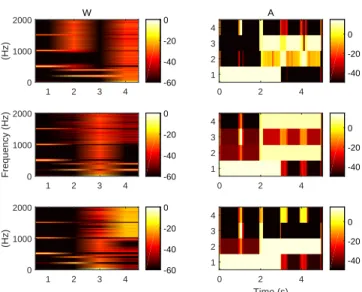
To illustrate how the HPNMF works (Algorithm 1), we use a simple synthetic signal. The test signal models a mix of harmonic and percussive components. The harmonic part is simulated by a sum of sine waves that overlap in time and frequency. The first signal simulates a C(3) with fun-damental frequency f0 = 131 Hz, the other one a B(4) with f0 = 492 Hz. To simulate the percussive part, we add 0.1 s of Gaussian white noise for the first two seconds. For the last two seconds, we add 0.3 s of Gaussian white noise filtered by a high-pass filter. The signal is 5 s long and the sampling rate is 4000 Hz. We compute the STFT with a 512 sample-long (0.128 s) Hann analysis window and a 50% overlap. The spectrogram of the signal is represented in Figure 1. As our input signal has four sources, we expect that one source can be represented by one component and therefore, that a model of rank 4 (k = 4) should adequately model the signals. More precisely, for the NMF and the PNMF we chose k = 4 and for the HPNMF the rank of the harmonic part is kH= 2 and the rank of the percussive part is kP = 2. The choice of the rank
of factorization is an important variable of the problem. In this case, we select it in order to illustrate the performance of the method. We will further discuss the importance of the choice of the rank of factorization in Section IV-D. We compare the HPNMF with the PNMF and the NMF using the KL distance with multiplicative update rules as stated in [46]. The three algorithms are initialized with the same random positive matrices Wini∈ Rn×k and Aini∈ Rk×m+ .
Time (s) Frequency (Hz) 0 0.5 1 1.5 2 2.5 3 3.5 4 4.5 5 0 200 400 600 800 1000 1200 1400 1600 1800 2000 −50 −40 −30 −20 −10 0 10
Fig. 1: Spectrogram of the synthetic test signal. The results of the decomposition are presented in Figure 2. The dictionary and activation matrices show the separation performance of the three methods. The NMF does not separate correctly the four components. By looking at the columns 2 and 3 of the dictionary matrix W in Figure 2, the filtered Gaussian white noise and the C(3) are separated in the same components which does not correspond to the expected result. For the PNMF, the orthogonal components do not succeed to represent the two noises correctly. They are extracted in the same component and the total reconstruction error of the PNMF is high. In this example, the HPNMF extracts the four components with the highest accuracy and is more efficient than the other methods. The two harmonic components are extracted in the orthogonal part (i.e., the columns 1 and 2 of the dictionary matrix) while the percussive components are extracted by the NMF part (columns 3 and 4). The HPNMF then outperforms the other two methods and shows the poten-tial of the proposed algorithm for harmonic/percussive source separation.
B. Protocol and Details of the Test Database of Real Signals We run several tests on the public SiSEC database from [47] to study the impact of the learned dictionaries in the HPNMF (Algorithm 2). This database is composed of polyphonic real-world music excerpts. Each music signal contains percussive and harmonic instruments as well as vocals. It consists of four recordings whose duration range from 14 to 24 s. Our goal is to perform a harmonic/percussive decomposition. Thus, following [10], we do not consider the vocal part and we build mixture signals only from the percussive and harmonic instruments. All the signals are sampled at 44.1kHz. We compute the STFT with a 1024 and 2048 sample-long Hann window with a 50% overlap. Four tests are run on these data: 1) The first test compares the HPNMF and the RegNMF in
Section IV-C. 1 2 3 4 0 1000 2000 (Hz) -60 -40 -20 0 0 2 4 Time (s) 1 2 3 4 -40 -20 0 W 1 2 3 4 0 1000 2000 (Hz) -60 -40 -20 0 A 0 2 4 1 2 3 4 -40 -20 0 1 2 3 4 0 1000 2000 Frequency (Hz) -60 -40 -20 0 0 2 4 1 2 3 4 -40 -20 0
Fig. 2: Results of the decomposition of the NMF (top), PNMF (middle) and HPNMF (bottom).
2) The second test aims at assessing the robustness of the HPNMF with respect to the rank of the PNMF part in Section IV-D.
3) The third test estimates which of the three divergences (Euc, KL and IS respectively) gives the best har-monic/percussive decomposition results in Section IV-E. 4) The last test shows the influence of the dictionary on the
separation performance in Section IV-F.
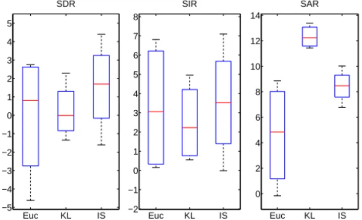
Note that the SiSEC database used for tuning the proposed method is different from the one in the evaluation phase in order to prevent any possible over-training. In order to evaluate and compare the results we then compute Signal to Distortion Ratio/Signal to Interference Ration/Signal to Artefact Ratio (SDR/SIR/SAR) that are common metrics for blind source separation with the BSS-Eval toolbox [48]. The SIR measures the rejection of interference between the two sources, the SAR measures the rejection of artefacts and finally the SDR measures the global separation quality.
C. Comparison Between the HPNMF and the Regularized NMF
Here the two methods are going to be tested using the same drum dictionary, with the same rank of factorization (the rank of factorization of the harmonic part is set to kH = 150) and the optimization is made with the IS divergence.
The HPNMF does not require further tuning whereas the two hyper-parameters of the regularized method (see Eq. (8)) need to be optimised on a development database. The develop-ment database was created using five songs from the Medley-dB [49]. The five songs were chosen in order to be acoustically homogeneous to the songs from the SiSEC database (2 pop songs, 2 rock songs, 1 rap song). This optimization process gives a set of values for the hyper-parameters that maximize the average SDR, SIR and SAR results. In our case we found that kT SM = 0.5 and kSSP = 0.2 were the most appropriate
set of hyper-parameters. However, it is not guaranteed that these fixed values maximize the score on each specific song. In Figure 3 each box-plot is made of a central line indicating the median of the data, upper and lower box edges indicating the 1st and 3rd quartiles while the whiskers indicate the minimum and maximum values. Figure 3 shows the results of the decomposition on the SiSEC database. The results of the HPNMF for the SDR and SIR are above the regularized NMF. The average SDR is about 0.8dB higher and the average SIR is more than 2dB greater.
Fig. 3: Decomposition results for the percussive (left bar)/harmonic (right bar) decomposition of the HPNMF and
the Regularized NMF on the SiSEC database. An explanation is that the parameters of the harmonic part on the RegNMF, although optimal on the development database, are not tuned to the test database. The values of the temporal regularity and spectral sparsity constraints are too low, and therefore, some of the percussive instruments are extracted in the harmonic part.
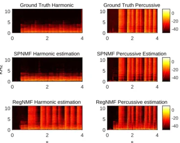
As an example, we display in Figure 4 the decomposition results between the RegNMF and the HPNMF. The harmonic estimation of the RegNMF is not accurate and some percussive components are present. The value for the parameters obtained on the development database are not optimal for this particular song. Here, the results of the percussive part are very similar between the two algorithms. As the dictionary used to decom-pose the data is the same for the two approaches, such results are to be expected. The RegNMF is overall less robust than the HPNMF.
D. Robustness with Respect to the Rank of the Harmonic Part In the HPNMF algorithm with a fixed drum dictionary, the only parameter is the rank of factorization of the harmonic part. In this experiment, we use the HPNMF algorithm with the fixed dictionary obtained from the STFT of a drum signal as described in Section III-E. The algorithms are implemented using the multiplicative update rules given in the appendix A, B and C and they are all initialized with the same random nonnegative matrices.
The average SDR values of the harmonic and percussive separation results are displayed in Figure 5 (results with
Ground Truth Harmonic
0 2 4
0 5 10
Ground Truth Percussive
0 2 4 0 5 10 -40 -20 0 SPNMF Harmonic estimation 0 2 4 0 5 10 KHz SPNMF Percussive Estimation 0 2 4 0 5 10 -40 -20 0
RegNMF Harmonic estimation
0 2 4
s
0 5 10
RegNMF Percussive estimation
0 2 4 s 0 5 10 -40 -20 0
Fig. 4: Comparison between the ground truth, the HPNMF and the RegNMF on the SiSEC database.
SIR/SAR exhibit similar behaviours and are therefore not displayed here). We can observe that when the rank of factor-ization is small (6 ≤ kH≤ 50), the Euclidean distance and the KL divergence do not give satisfactory results and it is only at kH>= 100 that they stabilize for both algorithms. With the IS divergence, the results seem to be more or less independent to the rank of factorization. This may be explained by the size and relative simplicity of the audio pieces of the SiSEC database. Indeed, the audio excerpts are short (≤ 30 seconds) and have a low rank harmonic content that is well represented with a few orthogonal basis functions.
0 100 200 300 400 500 Rank of factorization -2 -1 0 1 2 3 4 5 6 7 8 SDR (dB) Euclidean Kullback-Leiber Itakura-Saito
Fig. 5: Optimization of the rank of factorization with the three divergences (6 ≤ kH≤ 500).
Optimizing the HPNMF is a simple process because the method is robust to the rank of the harmonic part. For the rest of the article, the rank of factorization will be set to kH = 150 for all methods.
E. Influence of the Divergence
In this section we discuss the influence of the divergence in the results of the HPNMF algorithm. It has been estab-lished that the IS divergence is well suited for audio signal decomposition [50] as it is scale invariant. This means that the TF points with low energy of the spectrogram have the same relative importance as the high energy ones. This invariance is interesting for audio signals which have a wide dynamic range. Indeed music signals are composed of very localized components with low energy (transients) and quasi-sinusoidal parts of higher energy (tonal), which contribute both to the timbre and the perceived quality of the signal. However, it should be noted that it does not always lead to superior separation performance [10].
We here perform a comparison of the three divergences on the SiSEC database ( We also compare two different window lengths (1024 samples and 2048 samples) for the Fourier transform (see Figures 6 and 7).
Euc KL IS −10 −5 0 5 SDR Euc KL IS 1 2 3 4 5 6 7 8 9 10 11 SIR Euc KL IS −4 −2 0 2 4 6 8 10 12 14 16 SAR
Fig. 6: Average SDR, SIR and SAR of the estimated sources on the SiSEC database with a window size of 1024 samples.
Euc KL IS −5 −4 −3 −2 −1 0 1 2 3 4 5 SDR Euc KL IS −2 −1 0 1 2 3 4 5 6 7 8 SIR Euc KL IS 0 2 4 6 8 10 12 14 SAR
Fig. 7: Average SDR, SIR and SAR of the estimated sources on the SiSEC database with a window size of 2048 samples. The best results are obtained with the IS divergence and the window length of 2048 samples (see Figure 7) with +2dB in terms of SDR compared to the KL divergence and +1dB compared to the Euclidean distance. Similarly in terms of
SIR the results are around 1dB higher for the IS divergence compared to the other divergences.
Figure 6 shows that with a window of 1024 samples, the average separation scores are around 2dB below in terms of SDR and 1dB below in terms of SIR for the IS and KL divergence compared to the results of Figure 7. A smaller window size leads to a lower frequency resolution which lowers the separation scores as the percussive and harmonic components are not as well separated in the TF domain.
Thus, we will use the HPNMF algorithm with the IS divergence and a window size of 2048 samples for the STFT. F. Influence of the Dictionary
We discuss below the different methods used to construct the drum dictionary. As the dictionary is fixed, the estimation of the optimal learning parameters is crucial. In particular, it is important to find a good trade of for the size of the learning dataset to capture sufficient information to decompose any signal at a reasonable cost. Two types of audio recordings are available: the first type contains drum hits of the independent elements of the drum kit and the other type of audio files are drum phrases. For each drummer, we created three signals of different lengths (6 min, 12 min, 30 min) which gave us a total of 9 audio signals. Finally, we compute the STFT of these 9 signals and we execute a NMF on each of the spectrograms to obtain various dictionaries. The rank of the decomposition is chosen as 6 ≤ kP ≤ 500. In total, 108 dictionaries are created. Several tests are then carried out in order to evaluate the influence of:
• the dataset (drummer number 1, 2 or 3), • the length of the audio signal,
• the factorization rank.
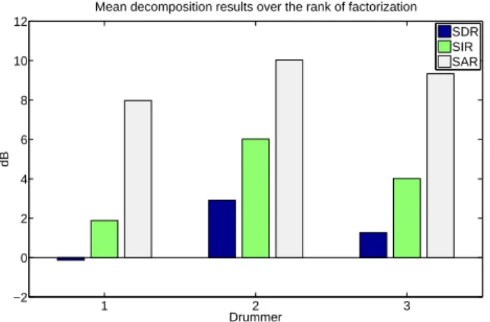
We show on the Figure 8 the SDR, SIR and SAR results averaged between the harmonic and percussive parts on all the factorization ranks for each drummer. We note that the results of the drummer 2 are the highest which may be explained by the fact that the drums sounds are here quite similar to the drums sounds found in the SiSEC recordings. The drummer 1 plays on a very small drum set the resulting dictionary does not contain enough information to well represent the instruments of the test signals. Conversely, the drummer 3 uses a large drum set with many elements that are not necessarily present in most recordings of the SiSEC database. The dictionary created is not sufficiently representative of the drum of the SiSEC songs.
In the remainder of this paper, all experiments are performed using the dictionaries built on the audio files of the drummer 2 dataset.
Figure 9 shows the influence of the length of the audio signals on the separation results. Above 6 min of training data, the quality of the decomposition decreases. In this case, it seems that when the training signals are too long, the dictio-nary created by the NMF become very specific to the training signal. In fact, the amount of information to decompose is too large and in order to minimize the reconstruction error (i.e., the value of the cost function), the NMF will favour the basis functions capturing the maximum energy possible. These
1 2 3 −2 0 2 4 6 8 10 12 dB Drummer
Mean decomposition results over the rank of factorization SDR SIR SAR
Fig. 8: Mean SDR SIR and SAR results averaged for each drummer on the SiSEC database.
6 12 30 0 2 4 6 8 10 12 dB Min
Mean decomposition results for the three differents lengths of signals SDR SIR SAR
Fig. 9: Mean SDR SIR and SAR results for the dictionaries learned with different signal lengths on the SiSEC database
(dictionary trained on drummer 2 data).
basis functions of the resulting dictionary do not contain drum-specific information, but rather atoms drum-specific to the training signal.
Finally, Figure 10 shows the results as a function of the rank of factorization. For kP > 100, the results in terms of SDR are close to 0dB. In this case the dictionary does not match the drums of the test songs and the harmonic and percussive sounds of the original signal are decomposed in the harmonic part of the HPNMF. This causes a high SAR because, although the decomposition is not satisfactory, the separated signals do not contain artifacts. In our tests, the optimal value of the rank of factorization is kP = 12. This value is specific of course to the records of the ENST-Drums [44] database and to our evaluation database (in this case, the SiSEC database).
For the rest of the article, we will use a dictionary con-structed using a 6 min long audio signal from the drummer 2 with kP = 12.
V. STATEOFTHEARTBENCHMARK
In this section, we compare the proposed method with the four state of the art methods presented in Section II-B on a large evaluation database. We first illustrate the database used for evaluation in Section V-A and then we describe the implementation of the state of the art methods used for
6 9 12 25 50 100 200 500 0 5 10 15 dB Rank of Factorization Mean decomposition results
SDR SIR SAR
Fig. 10: Mean SDR SIR and SAR results for various rank of factorization on the SiSEC database (dictionary trained on
drummer 2 data - 6 min long signals).
comparison in Section V-B. Section V-C details the results of the benchmark on the database while Section V-D presents the results on a sub-database. Finally, Section V-E outlines partial conclusions from the results.
A. Database
We use the Medley-dB [49] database that is composed of polyphonic real-world music excerpts. It contains 122 music signals, among which 89 of them contain percussive instru-ments. Because our goal is to perform a harmonic/percussive decomposition, the vocal part is omitted, following the same protocol as in [10]. All the signals are sampled at 44.1kHz.
In our tests, the training database of the HPNMF and the NMPCF are only composed of drums sounds. The database Medley-dB [49] contains a wide variety of percussive in-struments that are not in the training database ENST-Drums [44]. We will thus asses the robustness of the supervised methods when decomposing a signal that contains a percussive instrument that is not in the training database.
B. Implementation of the State of the Art Methods
The HPNMF with the fixed dictionary is bench-marked against the methods described in Section II-B: the CoNMF [10], the MF [9] the NMPCF [40] and the KAM [39]. We have re-implemented the CoNMF and the NMPCF and we have used the optimal parameters recommended by the authors in their respective articles. The MF and KAM implementations are taken from [51] and [39] respectively, and we used the standard parameters for a HPSS task.
C. Results
Table I shows the SDR, SIR and SAR results of the five methods on the selected 89 songs of the original Medley-dB database [49].
On average, the HPNMF and KAM obtain the highest separation scores compared to the other methods for the percussive, harmonic and mean SDR (≈ +1.5dB). The mean
HPNMF Harmonic Percussive Mean
SDR 4.5 -2.5 1.0
SIR 10.8 1.2 6.0
SAR 9.3 8.0 8.6
MF Harmonic Percussive Mean
SDR 3.5 -6.2 -1.3
SIR 7.5 0.5 4.0
SAR 8.9 -1.2 3.8
CoNMF Harmonic Percussive Mean
SDR 3.7 -4.8 -0.5
SIR 10.3 -3.3 3.5
SAR 6.3 8.1 7.2
NMPCF Harmonic Percussive Mean
SDR 3.5 -4.7 -0.6
SIR 8.9 -3.1 2.9
SAR 7.5 7.0 7.3
KAM Harmonic Percussive Mean
SDR 5.0 -3.0 1.0
SIR 8.2 6.6 7.4
SAR -0.1 13.6 6.7
TABLE I: SDR, SIR, SAR for percussive/left, harmonic/middle, mean/right separation results on the
database for the five methods.
SAR is +1.6dB higher for the HPNMF while the KAM achieves +1.4db mean SIR. The audio examples confirm the results as the separated sources from the KAM technique have a significant amount of artefacts. It should be noted that some songs of the database contain percussive instruments that are not present in the learning database ENST-Drums, such as the tambourine, the bongo, the gong and electronic drums. Because the dictionary is fixed, these percussive instruments are not correctly decomposed by the HPNMF. Some songs are well separated while others obtain much lower results since the percussive part is not well decomposed. These particular songs negatively impact the overall scores of our method.
The NMPCF, also based on trained data, is more robust than the HPNMF because the dictionary that extracts the drums is not fixed. It allows more flexibility and the results are more consistent even if some percussive instruments are not in the learning database. However, the mean score is lower than the proposed method. Moreover, the harmonic part in HPNMF is fully unconstrained and can capture percussive components which are not well described by the WP dictionary.
The results of the MF are lower than the other methods. A wide variety of harmonic instruments in the database have really strong transients and rich harmonic spectra (distorted electric guitar, glockenspiel etc.). Similarly, some percussive instruments have sparse basis functions localized in the low frequency range (bass drum, bongo, toms etc.), which can explain why the MF fails to extract these instruments in the appropriate harmonic/percussive parts. On average, it is able to correctly separate the percussive part (with relatively high SDR and the highest SIR), but it shows a very low SAR compared to the other methods. Similar outcomes have been observed in [10].
The CoNMF algorithm results are lower than those of the HPNMF. Some transients of the harmonic instruments are decomposed in the percussive part, and some percussive in-struments (mainly in the low frequency range) are decomposed in the harmonic part. The parameters used for the CoNMF are
not the optimal for the Medley-dB database. The value of the four parameters estimated in [10] are not tuned for a wide variety of audio signals.
Figure 11 shows the decomposition results on a specific song of the Medley-dB database. The parameters of the CoNMF are not tuned for this song and the algorithm does not extract the percussive and harmonic parts correctly. The NM-PCF and the MF still contain a significant amount of harmonic components in the percussive part. These two methods do not produce a clean separation. Finally, the HPNMF provide the best decomposition on this specific signal.
Harmonic Oracle 20 22 24 0 5 10 Percussive Oracle 20 22 24 0 5 10 HPNMF 20 22 24 0 5 10 HPNMF 20 22 24 0 5 10 CoNMF 20 22 24 0 5 10 CoNMF 20 22 24 0 5 10 Frequency (kHz) NMPCF 20 22 24 0 5 10 NMPCF 20 22 24 0 5 10 MF 20 22 24 0 5 10 MF 20 22 24 0 5 10 KAM 20 22 24 Time (s) 0 5 10 KAM 20 22 24 Time (s) 0 5 10
Fig. 11: Percussive (right)/Harmonic (left) ground truth and estimation results for the five methods (all the spectrogram
have the same amplitude range).
D. Results on a Genre Specific Database
The individual results on most of the songs of the database are similar to the average results. However, some interesting results were found on specific genres of music. Here we present the results on the 14 songs of the ”Electronic/Fusion” sub-database. These songs for the most part have a lot of silence and some solos played by only one instrument. Also, the electronic drum often repeats the same pattern during the
whole song resulting in a very redundant drum part. The SDR, SIR and SAR results on the sub-database are displayed in Table II.
The MF method gives competitive outcomes, with a low variance for the percussive estimation and a good overall mean. The MF obtains consistent results as well throughout the database and the decomposition on the genre specific database are significantly better than the ones on the whole database. It reflects the fact that the HPSS task from that musical genre is easier.
The results of the NMPCF are the lowest of the five meth-ods. The unconstrained harmonic part of the NMPCF extract most of the energy of the original signal and the information is unequally distributed in the harmonic and percussive layers. The CoNMF does not obtain satisfying results on the sub-database either. The parameters are estimated on a training database of another genre. Because of that, the value of the parameters are not set correctly and similarly to the NMPCF, the information is not distributed in the appropriate harmonic/percussive parts.
Finally, the KAM algorithm also under-performs on this genre specific database compared to HPNMF. More specifi-cally, the KAM method is particularly outperformed on silence segments and on solo-instrumental parts.
On the sub-database, the HPNMF clearly outperforms the other methods. Similarly to Section V-C, the percussive de-composition of the HPNMF has high variance because some of the instruments are not in the learning database. However, the mean of the percussive decomposition is significantly higher than the CoNMF and the NMPCF. Furthermore, the harmonic decomposition and the mean results of the HPNMF are clearly better than the ones of the other methods. The HPNMF is an effective algorithm to extract the redundant drum parts. Likewise, as the drum dictionary is fixed, it is unlikely the percussive part would be able to extract harmonic components. As the columns of WH are orthogonal, it is also unlikely for the harmonic part to extract percussive components. Contrary to the other algorithms, when the harmonic or percussive instruments are playing alone, the HPNMF does not extract any information in the percussive nor the harmonic parts.
E. Discussion
Each of the tested methods has its own advantages and drawbacks. The MF is the easiest and the fastest method to im-plement and it is relatively straightforward to tune. The results of the MF can be competitive when the harmonic instruments have smooth transients (i.e., sustained instruments such as the flute, the violin) and when the percussive instruments have flat spectra (i.e., cymbal, snare drum). However, when the harmonic instruments have strong transients (glockenspiel, piano) and the percussive instruments have sparse spectra (bass drum, bongo) the MF does not give good results.
The CoNMF is based on the same hypothesis than the MF and has the same issue. Fine tuning of the hyper-parameters can alleviate the problem mentioned above but it is a tedious process and is not possible in the case of blind source separation. Our tests on a large database show that the CoNMF
HPNMF Harmonic Percussive Mean
SDR 3.9 1.6 2.8
SIR 6.8 4.8 5.8
SAR 8.2 7.4 7.8
MF Harmonic Percussive Mean
SDR 1.2 -3.8 -1.3
SIR 2.7 3.7 3.2
SAR 8.5 -1.3 3.6
CoNMF Harmonic Percussive Mean
SDR 1.7 -1.6 0.1
SIR 4.7 -0.2 2.4
SAR 6.5 8.0 7.2
NMPCF Harmonic Percussive Mean
SDR 1.1 -1.4 -0.1
SIR 4.0 -0.1 1.9
SAR 5.9 8.0 7.0
KAM Harmonic Percussive Mean
SDR 1.5 -2.2 -0.3
SIR 3.6 6.5 5.0
SAR 9.8 1.5 5.7
TABLE II: SDR, SIR and SAR scores on the ”Electronic/Fusion” sub-database for the five methods.
is not robust enough for a wide variability of the analysed signals.
Contrary to the results obtained in [10], our evaluation on a larger dataset shows that the NMPCF algorithm gives competitive results compared to the MF and the constrained NMF. However, as it uses training to guide the decomposition process, it requires a wide variety of information to perform on a large scale test. If the training database cannot contain sufficient information, the results cannot be satisfying.
The KAM algorithm gives competitive results compared to the proposed method. However it is prone to excessive artefacts in the decomposition results which are more uncom-fortable to listen to2. Also the KAM is more computationally intensive than other methods an it require twice the time to process that same signal.
On a large scale test, the proposed method outperforms the other methods. It is able to extract the harmonic and the percussive instruments with higher scores for the SDR and SAR. Using prior dictionary learning with a physical model on the harmonic instruments thus helps to separate sources with much better accuracy even if similarly to [10] our method may suffer in the case of significant mismatch between the train and test subsets (e.g. in particular when some instruments are absent from the training subset).
VI. CONCLUSION
In this article, we have proposed a novel hybrid method built upon Nonnegative Matrix Factorisation NMF that decomposes the time frequency representation of an audio signal into a tonal part, estimated by a sparse and orthogonal nonnegative decomposition, and a transient part, estimated by a straight-forward NMF decomposition constrained by a pre-learned dictionary of smooth spectra.
An extensive evaluation on a large diverse database has demonstrated that the HPNMF is a very promising model for harmonic/percussive decomposition. Indeed, the HPNMF
outperforms four other state of the art methods on the medley-dB database [49]. A main advantage of the proposed method is that it is robust since it has very few hyperparameters to tune, and the optimization problem can be solved thanks to simple multiplicative update rules.
Another contribution of this work is that carrying out an evaluation on a large database allowed us to compare more accurately the performance of the four state-of-the-art methods on a large variety of music signals, and to get new insight about their potential for HPSS.
In future work, we plan to improve the dictionary learning process. We can say that the information from the drum dictionary built from the database ENST-Drums [44] is not sufficient to perform a harmonic/percussive source separation on a large scale. Depending on the style of music, some drums share similarities. A possible improvement would be to build genre specific drum dictionaries. In this way, the computation time would be reasonable as the amount of information could be reduced, and the templates of the dictionary could be a lot more focused on specific types of drums.
APPENDIX
A. Euclidean Distance
The euclidean distance gives us the problem: min
W1,W2,A2≥0
kV − W1W1TV + W2A2k2 The gradient with respect to W1 gives the update:
[∇W1D(V | ˜V )] − = 2V VTW 1 and [∇W1D(V | ˜V )] += 2V AT 2W T 2 W1+ W2A2VTW1+ V VTW1W1TW1+ W1W1TV VTW1 Similarly, the gradient with respect to W2 gives:
[∇W2D(V | ˜V )] −= V AT 2 and: [∇W2D(V | ˜V )] += 2W 1W1TV A T 2 + W2A2AT2 Finally, the gradient with respect to A2 gives:
[∇A2D(V | ˜V )] − = WT 2V and: [∇A2D(V | ˜V )] += 2WT 2W1W1TV + W T 2W2A2
B. Kullback Leiber Divergence
The Kullback Leiber divergence gives us the problem: min
W1,W2,A2≥0
V (log(V ) − log( ˜V )) + (V − ˜V ) The gradient with respect to W1 gives:
[∇W1D(V | ˜V )] − i,j= (ZV TW 1)i,j+ (V ZTW1)i,j with Zi,j = (W V
1W1TV +W2A2)i,j. The positive part of the
gradient is: [∇W1D(V | ˜V )] + i,j= X k (WTV )j,k+ ( X k Vi,k)( X a Wa,j)
Similarly, the gradient with respect to W2gives: [∇W2D(V | ˜V )] −= V AT 2 and: [∇W2D(V | ˜V )] += W 1W1TV A T 2 + W2A2AT2
Finally, the gradient with respect to A2 gives: [∇A2D(V | ˜V )] −= WT 2 V and: [∇A2D(V | ˜V )] += 2WT 2 W1W1TV + W T 2W2A2
C. Itakura Saito Divergence
The Itakura Saito divergence gives us the problem: min W1,W2,A2≥0 V ˜ V − log( V ˜ V) − 1. The gradient with respect to W1 gives:
[∇W1D(V | ˜V )] − i,j = (ZV TW 1)i,j+ (V ZTW1)i,j with Zi,j = (W V
1W1TV +W2A2)i,j. The positive part of the
gradient is: [∇W1D(V | ˜V )] + i,j= (φV T W1)i,j+ (V φTW1)i,j with φi,j = ( I W1W1TV + W2A2 )i,j
and I ∈ Rf ×t; ∀i, j Ii,j = 1.
Similarly, the gradient with respect to W2gives: [∇W2D(V | ˜V )] −= V AT 2 and: [∇W2D(V | ˜V )] += W 1W1TV A T 2 + W2A2AT2 Finally, the gradient with respect to A2 gives:
[∇A2D(V | ˜V )] −= WT 2 V and: [∇A2D(V | ˜V )] += 2WT 2 W1W1TV + W T 2W2A2
REFERENCES
[1] A. Ozerov, E. Vincent, and F. Bimbot, “A general flexible framework for the handling of prior information in audio source separation,” IEEE Transactions on Audio, Speech, and Language Processing, vol. 20, no. 4, pp. 1118–1133, 2012.
[2] J.-L. Durrieu, B. David, and G. Richard, “A musically motivated mid-level representation for pitch estimation and musical audio source separation,” IEEE Journal of Selected Topics in Signal Processing, vol. 5, no. 6, pp. 1180–1191, Oct. 2011.
[3] J. Salamon and E. Gomez, “Melody extraction from polyphonic music signals using pitch contour characteristics,” IEEE Transactions on Audio, Speech, and Language Processing, vol. 20, no. 6, pp. 1759–1770, Aug 2012.
[4] M. Ryynanen and A. Klapuri, “Automatic bass line transcription from streaming polyphonic audio,” in IEEE International Conference on Acoustics, Speech and Signal Processing (ICASSP), vol. 4, April 2007, pp. IV–1437–IV–1440.
[5] O. Gillet and G. Richard, “Transcription and separation of drum signals from polyphonic music,” IEEE Transactions on Audio, Speech, and Language Processing, vol. 16, no. 3, pp. 529–540, March 2008. [6] A. Roebel, J. Pons, M. Liuni, and M. Lagrangey, “On automatic drum
transcription using non-negative matrix deconvolution and itakura saito divergence,” in IEEE International Conference on Acoustics, Speech and Signal Processing (ICASSP), April 2015, pp. 414–418.
[7] S. B. Jebara, “Periodic/aperiodic decomposition for improving coherence based multi-channel speech denoising,” in 9th International Symposium on Signal Processing and Its Applications, Feb 2007, pp. 1–4. [8] B. Yegnanarayana, C. d’Alessandro, and V. Darsinos, “An iterative
algorithm for decomposition of speech signals into periodic and aperi-odic components,” IEEE Transactions on Speech and Audio Processing, vol. 6, no. 1, pp. 1–11, Jan 1998.
[9] D. Fitzgerald, “Harmonic/percussive separation using median filtering,” in International Conference on Digital Audio Effects (DAFx), 2010. [10] F. Canadas-Quesada, P. Vera-Candeas, N. Ruiz-Reyes, J. Carabias-Orti,
and P. Cabanas-Molero, “Percussive/harmonic sound separation by non-negative matrix factorization with smoothness/sparseness constraints,” EURASIP Journal on Audio, Speech, and Music Processing, vol. 2014, no. 1, pp. 1–17, 2014.
[11] J. Laroche, Y. Stylianou, and E. Moulines, “Hns: Speech modification based on a harmonic+noise model,” in IEEE International Conference on Acoustics, Speech and Signal Processing (ICASSP), vol. 2, April 1993, pp. 550–553 vol.2.
[12] B. Elie and G. Chardon, “Robust tonal and noise separation in presence of colored noise, and application to voiced fricatives,” in 22nd Inter-national Congress on Acoustics (ICA), Buenos Aires, Argentina, Sep. 2016.
[13] L. Daudet, “A review on techniques for the extraction of transients in musical signals,” in Computer Music Modeling and Retrieval. Springer, 2006, pp. 219–232.
[14] A. Klapuri, “Multipitch analysis of polyphonic music and speech signals using an auditory model,” IEEE Transactions on Audio, Speech, and Language Processing., vol. 16, no. 2, pp. 255–266, 2008.
[15] A. Eronen and A. Klapuri, “Musical instrument recognition using cepstral coefficients and temporal features,” in IEEE International Con-ference on Acoustics, Speech and Signal Processing (ICASSP), vol. 2, 2000, pp. II753–II756.
[16] M. Alonso, G. Richard, and B. David, “Accurate tempo estimation based on harmonic + noise decomposition,” EURASIP Journal on Advances in Signal Processing, vol. 2007, no. 1, p. 082795, 2006.
[17] J. Salamon and E. G´omez, “Melody extraction from polyphonic music signals using pitch contour characteristics,” Transactions on Audio, Speech, and Language Processing., vol. 20, no. 6, pp. 1759–1770, 2012. [18] F. Rigaud and M. Radenen, “Singing voice melody transcription using deep neural networks,” in International Conference on Music Informa-tion Retrieval (ISMIR), 2016.
[19] J. Paulus and T. Virtanen, “Drum transcription with non-negative spectrogram factorisation,” in European Signal Processing Conference (EUSIPCO), 2005, pp. 1–4.
[20] C. Wu and A. Lerch, “On drum playing technique detection in poly-phonic mixtures.” in International Conference on Music Information Retrieval (ISMIR), 2016, pp. 218–224.
[21] D. Lee and S. Seung, “Learning the parts of objects by nonnegative matrix factorization,” Nature, vol. 401, pp. 788–791, 1999.
[22] S. Ewert and M. M¨uller, “Score-informed source separation for music signals,” Multimodal music processing, vol. 3, pp. 73–94, 2012.
[23] N. Bertin, R. Badeau, and G. Richard, “Blind signal decompositions for automatic transcription of polyphonic music: NMF and K-SVD on the benchmark,” in IEEE International Conference on Acoustics, Speech and Signal Processing (ICASSP), vol. 1, 2007, pp. 65–68.
[24] R. Hennequin, R. Badeau, and B. David, “Time-dependent parametric and harmonic templates in non-negative matrix factorization,” in Interna-tional Conference on Digital Audio Effects (DAFx), 2010, pp. 246–253. [25] J. Durrieu, G. Richard, B. David, and C. F´evotte, “Source/filter model for unsupervised main melody extraction from polyphonic audio signals,” IEEE Transactions on Audio, Speech, Language Process., vol. 18, no. 3, pp. 564–575, 2010.
[26] S. A. Raczy´nski, N. Ono, and S. Sagayama, “Multipitch analysis with harmonic nonnegative matrix approximation,” in International Confer-ence on Music Information Retrieval (ISMIR), 2007.
[27] A. Cichocki, R. Zdunek, A. H. Phan, and S.-i. Amari, Nonnegative matrix and tensor factorizations: applications to exploratory multi-way data analysis and blind source separation. John Wiley & Sons, 2009. [28] X. Jaureguiberry, P. Leveau, S. Maller, and J. J. Burred, “Adaptation of source-specific dictionaries in non-negative matrix factorization for source separation,” in IEEE International Conference on Acoustics, Speech and Signal Processing (ICASSP), 2011, pp. 5–8.
[29] C.-W. Wu and A. Lerch, “Drum transcription using partially fixed non-negative matrix factorization,” in European Signal Processing Confer-ence (EUSIPCO), 2008.
[30] T. Virtanen, “Monaural sound source separation by nonnegative matrix factorization with temporal continuity and sparseness criteria,” IEEE Transactions on Audio, Speech, Language Processing., vol. 15, no. 3, pp. 1066–1074, 2007.
[31] A. Hayashi, H. Kameoka, T. Matsubayashi, and H. Sawada, “Non-negative periodic component analysis for music source separation,” in Signal and Information Processing Association Annual Summit and Conference (APSIPA), 2016 Asia-Pacific. IEEE, 2016, pp. 1–9. [32] S. Choi, “Algorithms for orthogonal nonnegative matrix factorization,”
in IEEE International Joint Conference on Neural Networks (IJCNN), 2008, pp. 1828–1832.
[33] Z. Yang and E. Oja, “Linear and nonlinear projective nonnegative matrix factorization,” IEEE Transactions on Neural Network., vol. 21, no. 5, pp. 734–749, 2010.
[34] F. Rigaud, M. Lagrange, A. R¨obel, and G. Peeters, “Drum extraction from polyphonic music based on a spectro-temporal model of percussive sounds,” in IEEE International Conference on Acoustics, Speech and Signal Processing (ICASSP), 2011, pp. 381–384.
[35] J. Park, J. Shin, and K. Lee, “Exploiting continuity/discontinuity of basis vectors in spectrogram decomposition for harmonic-percussive sound separation,” IEEE/ACM Transactions on Audio, Speech, and Language Processing, vol. 25, no. 5, pp. 1061–1074, 2017.
[36] A. Liutkus, D. Fitzgerald, Z. Rafii, B. Pardo, and L. Daudet, “Kernel additive models for source separation,” IEEE Transactions on Signal Processing, vol. 62, no. 16, pp. 4298–4310, 2014.
[37] A. Bregman, Auditory Scene Analysis, The perceptual Organization of Sound. MIT Press, 1990.
[38] W. S. Cleveland and S. J. Devlin, “Locally weighted regression: an approach to regression analysis by local fitting,” Journal of the American statistical association, vol. 83, no. 403, pp. 596–610, 1988.
[39] D. FitzGerald, A. Liukus, Z. Rafii, B. Pardo, and L. Daudet, “Har-monic/percussive separation using kernel additive modelling,” in 25th IET Irish Signals Systems Conference 2014 and 2014 China-Ireland International Conference on Information and Communications Tech-nologies (ISSC 2014/CIICT 2014), June 2014, pp. 35–40.
[40] M. Kim, J. Yoo, K. Kang, and S. Choi, “Nonnegative matrix partial co-factorization for spectral and temporal drum source separation,” Journal of Selected Topics in Signal Processing, vol. 5, no. 6, pp. 1192–1204, 2011.
[41] Z. Yuan and E. Oja, “Projective nonnegative matrix factorization for image compression and feature extraction,” Image Analysis, pp. 333– 342, 2005.
[42] C. Laroche, M. Kowalski, H. Papadopoulos, and G. Richard, “A structured nonnegative matrix factorization for source separation,” in European Signal Processing Conference (EUSIPCO), 2015.
[43] D. Lee and S. Seung, “Algorithms for non-negative matrix factoriza-tion,” in Annual Conference on Neural Information Processing Systems (NIPS), 2001, pp. 556–562.
[44] O.Gillet and G.Richard, “Enst-drums: an extensive audio-visual database for drum signals processing.” in International Conference on Music Information Retrieval (ISMIR), 2006, pp. 156–159.
[45] A. Liutkus and R. Badeau, “Generalized Wiener filtering with fractional power spectrograms,” in IEEE International Conference on Acoustics, Speech and Signal Processing (ICASSP), 2015.
[46] C. F´evotte, N. Bertin, and JL.Durrieu, “Nonnegative matrix factorization with the itakura-saito divergence: With application to music analysis,” Neural Computation, vol. 21, no. 3, pp. 793–830, 2009.
[47] S. Araki, A. Ozerov, V. Gowreesunker, H. Sawada, F. Theis, G. Nolte, D. Lutter, and N. Duong, “The 2010 signal separation evaluation campaign : audio source separation,” in International Conference on Latent Variable Analysis and Signal Separation (LVA/ICA), 2010, pp. 114–122.
[48] E. Vincent, R. Gribonval, and C. F´evotte, “Performance measurement in blind audio source separation,” IEEE Transactions on Audio, Speech, Language Process., vol. 14, pp. 1462–1469, 2006.
[49] R. Bittner, J. Salamon, M. Tierney, M. Mauch, C. Cannam, and J. Bello, “Medleydb: A multitrack dataset for annotation-intensive mir research,” in International Conference on Music Information Retrieval (ISMIR), 2014.
[50] R. M. Gray, A. Buzo, A. H. Gray Jr, and Y. Matsuyama, “Distortion measures for speech processing,” Transactions on Acoustics, Speech and Signal Processing., vol. 28, no. 4, pp. 367–376, 1980.
[51] J. Driedger and M. M¨uller, “Tsm toolbox: Matlab implementations of time-scale modification algorithms,” in International Conference on Digital Audio Effects (DAFx), 2014, pp. 249–256.