HAL Id: hal-01008739
https://hal.archives-ouvertes.fr/hal-01008739
Submitted on 25 Mar 2020HAL is a multi-disciplinary open access archive for the deposit and dissemination of sci-entific research documents, whether they are pub-lished or not. The documents may come from teaching and research institutions in France or abroad, or from public or private research centers.
L’archive ouverte pluridisciplinaire HAL, est destinée au dépôt et à la diffusion de documents scientifiques de niveau recherche, publiés ou non, émanant des établissements d’enseignement et de recherche français ou étrangers, des laboratoires publics ou privés.
Recent Advances in Material Homogenization
Hajer Lamari, Amine Ammar, Patrice Cartraud, Francisco Chinesta, Frédéric
Jacquemin, Grégory Legrain
To cite this version:
Hajer Lamari, Amine Ammar, Patrice Cartraud, Francisco Chinesta, Frédéric Jacquemin, et al.. Recent Advances in Material Homogenization. 13th ESAFORM Conference on Material Forming, 2010, Brechia, Italy. �10.1007/s12289-010-0913-y�. �hal-01008739�
____________________
* Hajer Lamari: GEM, Centrale nantes, 1 rue de la Noe, BP 92101, F-44321 Nantes cedex 3, France, [email protected]
RECENT ADVANCES IN MATERIAL HOMOGENIZATION
H. Lamari
1*, A. Ammar
2, P. Cartraud
1F. Chinesta
1, F. Jacquemin
3, G. Legrain
11
GEM, Centrale Nantes, 1 rue de la Noe, BP 92101, F-44321 Nantes cedex 3, France
2
Laboratoire de Rhéologie, 13 rue de la Piscine, BP 53, F-38041 Grenoble cedex 9, France
3
GEM, Université de Nantes, 58, rue Michel Ange, BP 420, F-44606 Saint Nazaire cedex, France
ABSTRACT: Heterogeneous materials involve different length scales in their mechanical properties. Obviously a
mechanical description taking into account all the microscopic details is impossible from a computational point of view except for parts of very small dimensions. The main aim of material homogenization is defining macroscopic homogeneous properties able to represent at the macroscopic scale the real material and allowing for ignoring the microscopic scale in the numerical representation.
KEYWORDS: Homogenization, Model reduction, Separated representations, Proper Generalized Decompositions,
Parametric models.
1 INTRODUCTION
The interest and issues of material homogenization are today well established. Two important recurrent issues concern the definition of homogenized properties when the microstructure evolves from one point to other at the macroscopic scale, that is, throughout the macroscopic part. This evolution of the microstructure needs the definition of a homogenized model at each node (or integration point) in the macroscopic part, even in the linear case. The second issue concerns precisely the eventual non-linearity of thermomechanical properties. In that case moreover, one should solve a homogenization problem at each location throughout the part as well as at each time step because the evolution of microscopic properties with the model solution itself. In this work we present a technique able to alleviate the difficulty related to the evolution of the microstructure in the macroscopic scale. This technique is based on the consideration of a representative volume element consisting of different cells whose properties will be introduced as extra-coordinates of the thermo-mechanical model. Thus, the original thermo-thermo-mechanical model is transformed into a multi-dimensional parametric model suffering the redoubtable curse of dimensionality illness. The use of the proper generalized decomposition – PGD - allows circumventing this difficulty [1,2]. Section 2 revisits the application of PGD on parametric models. Some preliminary results involving heterogeneous linear thermal behaviours, perfectly defined at the microscopic scale, will be presented and discussed in section 3.
2 THERMAL PARAMETRIC MODEL
In this section we illustrate the application of the Proper Generalized Decomposition for solving a parametric thermal model involving a single extra-coordinate, the thermal conductivity characterizing an isotropic homogenous medium. This procedure will be extended later for including many extra-coordinates.
Consider the heat transfer equation:
0
u
k u
f
t
(1)where
( , , )
x
t k
I
and for the sake of simplicity the source term is assumed constant, i.e.f
cte
. Because the conductivity is considered unknown, it is assumed as a new coordinate defined in the interval
. Thus, instead of solving the thermal model for different values of the conductivity parameter we prefer introducing it as a new coordinate. The price to be paid is the increase of the model dimensionality; however, as the complexity of the PGD scales linearly with the space dimension the consideration of the conductivity as a new coordinate allows for faster and cheaper solutions.The solution of Eq. (1) is searched under the form:
1, ,
i N i i i iu
t k
X
T t
K k
x
x
(2)In what follows we are assuming that the approximation at iteration n is already done:
1, ,
i n n i i i iu
t k
X
T t
K k
x
x
(3)and at present iteration we look for the next functional product
X
n1
x
T
n1
t
K
n1
k
that for alleviating the notation will be denoted by
R
x
S t W k
. Prior to solve the resulting nonlinear model related to the calculation of these three functions a model linearization is compulsory. The simplest choice consists in using an alternating directions fixed point algorithm. It proceeds by assuming
S t
andW k
given at the previous iteration of the non-linear solver and then computingR x
. From the just updatedR x
andW k
we can updateS t
, and finally from the just computedR x
andS t
we computeW k
. The procedure continues until reaching convergence. The converged functionsR x
,S t
andW k
allow defining the searched functions:
1 nX
x
R
x
,T
n1
t
S t
and
1 nK
k
W k
.We are illustrating each one of the just referred steps:
I. Computing
R x
fromS t
andW k
:We consider the global weak form of Eq. (1):
*
0
Iu
u
k u
f
d dt dk
t
x
(4)where the trial and test functions write respectively:
1, ,
i n i i i iu
t k
X
T t
K k
R
S t W k
x
x
x
(5) and
* *, ,
u
x
t k
R
x
S t W k
(6)Introducing (5) and (6) into (4) it results:
* * ( ) I n I S R S W R W k R S W d dt dk t R S W d dt dk
x x (7) with ( ) 1 1 i n i n n i i i i i i i i T X K k X T K f t
.Now, being known all the functions involving the time and the parametric coordinate, we can integrate Eq. (7) in their respective domains
I
. Integrating inI
and taking into account the notation2 2 2 1 1 1 2 2 2 2 3 3 3 4 4 4 5 5 5 I I I i i i i i i I i i i i i i I w W dk s S dt r R d dS w kW dk s S dt r R R d dt w W dk s S dt r R d dT w W K dk s S dt r R X d dt w kW K dk s S T dt r R X d
x x x x x (8)Eq. (7) reduces to:
* 1 2 2 1 * 4 4 5 5 3 3 1 1 i n i n i i i i i i i i R w s R w s R d R w s X w s X w s f d
x x (9) Eq. (9) defines an elliptic steady state boundary value problem that can be solved by using any discretization technique operating on the model weak form (finite elements, finite volumes …). Another possibility consists in coming back to the strong form of Eq. (9):1 2 2 1 4 4 5 5 3 3 1 1 i n i n i i i i i i i i w s R w s R w s X w s X w s f
(10)that could be solved by using any collocation technique (finite differences, SPH …).
II. Computing
S t
fromR x
andW k
:In the present case the test function writes:
* *
, ,
u
x
t k
S
t
R
x
W k
(11)Now, the weak form reads
* * (n) I I S S R W R W k R S W d dt dk t S R W d dt dk
x x (12) that integrated in the domain
and taking into account the notation (8) results:* 1 1 2 2 * 4 5 5 4 3 3 1 1 I i n i n i i i i i i i i I dS S w r w r S dt dt dT S w r w r T w r f dt dt
(13) Eq. (13) represents the weak form of the ODE defining the time evolution of the field S that can be solved by using any stabilized discretization technique (SU, Discontinuous Galerkin, …). The strong form of Eq. (13) reads:1 1 2 2 4 5 5 4 3 3 1 1 i n i n i i i i i i i i
dS
w r
w r S
dt
dT
w r
w r T
w r
f
dt
(14) than can be solved by using backward finite differences, or higher order Runge-Kutta schemes, among many other possibilities.III. Computing
W k
fromR x
andS t
:In the present case the test function writes:
* *
, ,
u
x
t k
W
t
R
x
S k
(15)Now, the weak form reads
* * (n) I I S W R S R W k R S W d dt dk t W R S d dt dk
x x (16) that integrated in
I
and taking into account the notation (8) results:
* 1 2 2 1 * 5 4 4 5 3 3 1 1 i n i n i i i i i i i i W r s W r s k W dk W r s K r s k K r s f dk
(17) Eq. (17) does not involve any differential operator. The strong form of Eq. (17) reads:
1 2 2 1 5 4 4 5 3 3 1 i n i i i i i ir s
r s
W
r s
r s
K
r s
f
(18)that represents an algebraic equation. Thus, the introduction of parameters as additional model coordinates has not a noticeable effect in the computational cost, but can increase the number of sums involved in finite sums decomposition (2).
There are other minimization strategies more robust and exhibiting faster convergence for building-up the PGD (see [3]).
3 NUMERICAL EXAMPLES
In this section we are focusing in the thermal models defined in heterogeneous materials. Imagine a composite material involving a matrix and a fibrous reinforcement. A typical representative volume showing the microstructure heterogeneity is depicted in figure 1.
Figure 1. Microstructure of a composite material
Now, in order to apply the PGD one should perform a separated representation of the thermal conductivity, allowing for an efficient thermal simulation, i.e.
1( )
( )
P i i x y ik
K x K
y
x
(19)This separated representation can be performed by applying the SVD (singular value decomposition) to the matrix containing as entries the image pixels.
However, because the irregular distribution of the inclusions the number of sums in (19) becomes very high. Different possibilities exist to alleviate this representation some of them are being analyzed at present. A first possibility lies in considering only a reduced number of the modes of the SVD. The computational cost is significantly reduced and sometimes the precision is not too much degraded. Figure 2 depicts the image reconstruction for different number of sums in (20).
Figure 2. Reconstructed microstructure for
P
23
(left) andP
46
in (19).Another possibility lies in the substitution of each cercle by a square parallel to the coordinate axes, whose area equals the one of the associated circle. Eq. (20) represents a generic rectangle:
x x
a,
b
y y
a,
b
x
(20)Now, we define the characteristic function:
,0
1
0
a bif
s
a
s
if
a
s
b
if
s
b
(21)Using this notation, the square defined in (20) can be represented in a separated form by:
, ,
a b a b
x x
x
y yy
.Obviously, if the representative volume contains P inclusions, each one represented by a square, the separated representation (19) will contain P sums.
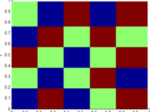
Obviously, all these approaches imply the solution of a thermal model for each representative volume (as soon as the microstrucvture evolve, the thermal conductivity is modified and then a new solution of the thermal model is required). If we consider a stochastic nature of the microstructure many realizations of the microstructure must be solved. One possibility for alleviating this task consists of considering the representative volume composed of a certain number of cells related to a grid of the representative volume as depicted in figure 3. Now, rather than solving a thermal model for each existing microstructure (represented by the different values of the thermal conductivity in each cell), we are introducing the thermal conductivity of each cell as an extra coordinate. In the example depicted in Fig. 3 the model will be defined in a space of dimension 27 (the x and y space coordinates and the
5 5
cells thermal conductivities).Figure 3. Cellular microstructure of the representative
volume element.
Thus, the solution is searched under the form:
1,1 5,5 1,1 1,1 5,5 5,5 1( , ,
,
,
)
( )
(
)
(
)
N i i i i iu x y k
k
X x Y y
K
k
K
k
L
L
(22)Thus, the thermal field for any possible microstructure only needs the solution of only one multidimensional problem, solution that can be performed efficiently by applying the PGD. As soon as the solution (22) is computed, the thermal field for any microstructure realization is obtained by substituting the known conductivities of each cell in Eq. (22). Thus, the thermal field related to the microstructure shown in Fig. 3 is depicted in Fig. 4 (a simple boundary condition
1,1 5,5
(
,
,
,
)
u
x
k
L
k
x
was enforced)Figure 4. Thermal field associated with the
microstructure depicted in Fig. 3.
4. CONCLUSIONS
This paper explores some possibilities related to the use of Proper Generalized Decomposition in the advanced simulation. This novel discretization technique allows the efficient solution of highly multidimensional models by circumventing the redoubtable curse of dimensionality that mesh based discretization techniques suffer.
As soon as an efficient solver for multidimensional models is available, many models of computational mechanics can be rewritten in higher dimensional spaces. Thus, one could for example compute the thermal field for any value of the thermal conductivity (as illustrated in this paper for homogeneous and heterogenous materials) simplifying inverse identification of optimization.
REFERENCES
[1] A. Ammar, B. Mokdad, F. Chinesta, R. Keunings, A new family of solvers for some classes of multidimensional partial differential equations encountered in kinetic theory modeling of complex fluids, J. Non-Newtonian Fluid Mech., 139: 153-176, 2006.
[2] A. Ammar, B. Mokdad, F. Chinesta, R. Keunings, A new family of solvers for some classes of multidimensional partial differential equations encountered in kinetic theory modeling of complex fluids. Part II: transient simulation using space-time separated representations, J. Non-Newtonian Fluid
Mech., 144: 98-121, 2007.
[3] F. Chinesta, A. Ammar, E. Cueto Recent Advances in the Use of the Proper Generalized Decomposition for Solving Multidimensional Models. Archives of Computational Methods in