HAL Id: hal-01857307
https://hal.archives-ouvertes.fr/hal-01857307
Submitted on 14 Aug 2018
HAL is a multi-disciplinary open access
L’archive ouverte pluridisciplinaire HAL, est
Real-time direct integration of reduced solid dynamics
equations
David González, Elías Cueto, Francisco Chinesta
To cite this version:
David González, Elías Cueto, Francisco Chinesta. Real-time direct integration of reduced solid
dy-namics equations. International Journal for Numerical Methods in Engineering, Wiley, 2014, 99 (9),
pp.633-653. �10.1002/nme.4691�. �hal-01857307�
Real-time direct integration of reduced solid dynamics equations
David Gonz´alez
1, El´ıas Cueto
1,∗, Francisco Chinesta
2,31Arag´on Institute of Engineering Research (I3A). Universidad de Zaragoza. Spain. 2Ecole Centrale de Nantes. France.´
3Institut Universitaire de France.
SUMMARY
A new method is developed here for the real-time integration of the equations of solid dynamics based on the use of POD-PGD approaches and direct time integration. The method is based upon the formulation of solid dynamics equations as a parametric problem, depending on their initial conditions. A sort of black-box integrator is obtained that takes the resulting displacement field of the current time step as input and (via POD) provides the result for the subsequent time step at feedback rates on the order of 1 kHz. To avoid the so-called curse of dimensionality produced by the large amount of parameters in the formulation (one per degree of freedom of the full model) a combined POD-PGD strategy is implemented. Examples are included that show the promising results of this technique.
KEY WORDS: Solid dynamics, PGD, POD, model order reduction, real-time simulation.
Contents
1 Introduction 2
2 Solid dynamics 4
3 Parametric, multidimensional, form of the problem 4
4 PGD approximation to parametric solid dynamics 5
4.1 High-dimensional approximation. . . 5
4.2 Example 1: Frame structure. . . 7
4.3 Example 2: Vibration of a clamped beam. . . 8
5 Parametrization of the space of initial conditions 10
5.1 A POD-PGD approach . . . 11
∗Correspondence to: El´ıas Cueto. Universidad de Zaragoza. Edificio Betancourt. Mar´ıa de Luna, s..n. E-50018 Zaragoza, Spain.
e-mail: [email protected]
6 Numerical Examples 12
6.1 Wave propagation on a block . . . 12
6.2 Including non-linear strain measures . . . 15
6.3 Palpation of a liver . . . 20
7 Conclusions 22
1. Introduction
Despite the well-known (and very often mentioned) growth in computer capabilities, some engineering problems still constitute today an intensive task. Structural dynamics is one of these problems, where the set of differential equations describing the system is usually discretized in space by finite elements (leading to an ODE in time) and then explicit or implicit methods in time are used to further discretize this ODE. This results in a system of very large number of degrees of freedom if fine enough meshes are employed in space, and (specially for explicit approaches) small-enough time steps are employed to avoid instability issues.
For this reason, structural dynamics has been one of the first fields of engineering practice where model order reduction has been employed. Classical modal analysis can be seen as a sort of model order reduction while, for instance, [32] seems to have been the first in employing eigenmodes of the structure with the purpose of reducing the number of degrees of freedom in non-linear applications. In essence, (projection-based) model order reduction consists in changing the original degrees of freedom of the model (i.e., finite element mesh nodal displacements) by an as much as possible reduced number of generalized variables that describe adequately the large-scale structures dominating the solution of the problem [29]. Recently, a number of works have pursued this same idea in the field of solid dynamics, see, to name a few, [38] [19] [21] [25] [45]. In these last works it is shown that model order reduction allows not only for a significant reduction of the number of spatial degrees of freedom, but also for larger time steps verifying stability constraints. However, in these references, an implicit simulation of 1.5 seconds of real time consumes 8540 seconds of computing time. Even if savings on the order of ten times have been reported for a judicious choice of the number of degrees of freedom, this is still far from real-time constraints.
Some applications are specially demanding for feedback responses of structural dynamics simulations. For instance, it is well known that haptic (force) peripherals require feedback responses on the order of 500 Hz to 1 kHz. This is equivalent to solve non-linear solid dynamics each millisecond, or one thousand times per second. To the best of our knowledge, only linear elastic models undergoing large deformations (Saint Venant-Kirchhoff models) have been solved under such an astringent requirement by employing either GPUs [43] or explicit algorithms combined with model reduction [44] [7] [6]. The extension of these techniques to account for the stability provided by implicit time integrators and general non-linear models seems to be difficult, even for reduced order models.
In this work a completely different (yet still based on some form of model order reduction) philosophy is employed. A computational vademecum [11] is developed that acts as a time integrator. This sort of black box is fed with the results of the previous time step, t, (in the form of the vector of nodal displacements of the model) and provides, under the severe feedback restrictions commented before, the solution at time t+4t, still providing the stability features of your preferred time integrator, implicit or not.
problem in a parametric framework. This means that the vector of displacements at time t is considered as parameters of the problem (in addition to being the initial conditions of the subsequent time step), the displacements at time t + 4t being the unknowns. Of course, the number of degrees of freedom in a nowadays problem of industrial interest is huge, so the number of parameters could be simply unaffordable. To alleviate this problem, a reduced order basis, obtained via Proper Orthogonal Decomposition (POD) [20] [27] [40] [42][41] is employed, thus guaranteeing the parametrization of the space of initial conditions with a minimum of degrees of freedom. Even with this efficient approach for the initial conditions, the number of parameters (initial conditions) usually reaches some tens.
The method is then structured in an off-line/on-line strategy. The parametric problem, depending on the initial conditions in the interval (t, t + 4t) is then solved off-line, and once for life, for any value of the parameters within a prescribed interval. This parametric problem can be solved by using your favorite time integrator, implicit or explicit, and the time step for these integrators need not to be the same 4t (can be smaller if, for some applications, the feedback response requirement is bigger than the stability constraints of the particular integrator used). Once this off-line phase of the method is computed (as already mentioned, only once for life), the on-line part can run under severe real-time constraints by simply feeding the “vademecum” with the results at the previous converged time step.
The only conceptual difficulty in this approach is to solve the parametric problem. Note that this problem considers every degree of freedom of the (reduced) model as a parameter. Thus, it is frequent to consider some tens of parameters for large (full) problems comprising thousands of finite element degrees of freedom. It is well-known that it is not possible to solve this kind of parametric problems by simply employing any mesh-based technique (finite elements, finite differences), since the number of degrees of freedom increases exponentially with the number of state space dimensions (equal to the number of spatial dimensions plus the number of parameters) [26].
To alleviate this curse of dimensionality, the authors, among others, have developed a technique coined as Proper Generalized Decomposition (PGD) [5] [4] [10] [12] [3] [16][15] that approximates the solution as a finite sum of separable functions. These functions are determined in the off-line part of the method by invoking a greedy algorithm (whose solution involves a non-linear problem, usually solved by simple fixed-point, alternate directions algorithm). The method, whose roots can be traced back to the space-time separation in the so-called radial loading technique within the LATIN method [22] [23] [24] [39][17], allows for an efficient solution of problems defined in high dimensional parameter spaces. In the PGD framework, the complexity of the problem scales linearly with the number of state space dimensions (parameters, actually), instead of exponentially.
With all these ingredients, that will be detailed in the sequel, the method here proposed provides with a sort of meta-model or surface response (computational vademecum, in words of [11]) of the system subjected to any type of force and initial conditions (taking values in a given interval).
The outline of the paper is as follows. In Section 2 we describe the basics of the formulation of the problem of solid dynamics here addressed. In Section3 the parametric form of the problem is introduced as a pre-requisite for the establishment of the off-line phase of the method. Section
4 develops the PGD-based formulation of the resulting multi-dimensional problem while Section5
explains how to obtain an efficient parametrization of the space of initial conditions. Finally, Section
6includes some numerical examples showing the potentiality of the proposed method. The paper is completed with some conclusions and comments on future works.
2. Solid dynamics
The strong form of the problem of solid dynamics is well-known, but it is reviewed here for completeness. We consider first the linear elastic case. Non linear strain measures will be analyzed in Section 6.2. For the former case the problem can be stated as: given f , g, h, u0 and ˙u0, find u : ¯Ω×]0, T ] → R3such that ρ ¨u = ∇ · σ + f in Ω×]0, T ] (1a) u = g on Γu×]0, T ] (1b) σn = h on Γt×]0, T ] (1c) u(x, 0) = u0(x) x ∈ Ω (1d) ˙ u(x, 0) = ˙u0(x) x ∈ Ω. (1e)
The corresponding weak form is: given f , g, h, u0 and ˙u0 find u(t) ∈ St = {u|u(x, t) = g(x, t), x ∈ Γu, u ∈ H1(Ω)}, t ∈ [0, T ], such that for all w ∈ V{u|u(x, t) = 0, x ∈ Γu, u ∈ H1(Ω)},
(w, ρ ¨u) + a(w, u) = (w, f ) + (w, h)Γ (2a)
(w, ρu(0)) = (w, ρu0) (2b)
(w, ρ ˙u(0)) = (w, ρ ˙u0), (2c) where we have used the so-called direct notation:
a(w, u) = Z Ω ∇sw : C : ∇su dΩ, (w, f ) = Z Ω wf dΩ, (w, h)Γ = Z Γt whdΓ.
This constitutes the main ingredient for a finite element semi-discretization of the problem, leading to an ODE to be discretized in time by your favorite time integrator, implicit or explicit. The method here proposed proceeds by stating the problem (2) in a parametric form. In this case, the parameters will be the initial conditions.
3. Parametric, multidimensional, form of the problem
The main modification in the standard approach to the problem given by Eqs. (1)-(2) is to reinterpret the parametric dependence of the problem on its initial conditions u0and ˙u0(assumed for the time being constant; the general case will be addressed later on) as being actually multi-dimensional:
where I = [u−0, u+0] and J = [ ˙u−0, ˙u+0] represent the considered intervals of variation of initial boundary conditions, u0and ˙u0. This makes it necessary to define a new (triply-) weak form where:
a(w, u) = Z I Z J Z Ω ∇sw : C : ∇su dΩd ˙u0du0, (w, f ) = Z I Z J Z Ω wf dΩd ˙u0du0, (w, h)Γ= Z I Z J Z Γt wh dΓd ˙u0du0.
With this modification in mind, one can proceed as in standard textbooks of finite elements and semi-discretize, with the help of appropriate finite-dimensional approximations to Stand V, Sthand Vh, respectively, the weak form so as to obtain the following problem: given f , g, h, u
0and ˙u0find uh(t) = vh+ gh∈ Sh
t (note that g(x, t) = u(x, t) on Γu) such that for every wh∈ Vh,
(wh, ρ¨vh) + a(wh, v) = (wh, f ) + (wh, h)Γ− (wh, ρ¨gh) − a(wh, gh), (5a) (wh, ρvh(0)) = (wh, ρu0) − (wh, ρgh(0)), (5b) (wh, ρ ˙vh(0)) = (wh, ρ ˙u0) − (wh, ρ ˙gh(0)). (5c)
This results in an absolutely general solution (thus the name computational vademecum coined in [11]) to the problem (2) for any initial conditions. A similar philosophy, but for simpler problems was implemented in [15]. It can also be viewed as a sort of response surface or meta-model obtained in an entirely computational way and in one execution of the algorithm. The method here developed computes off-line and once for life this general solution so as to be able to simply post-process during the on-line phase of the algorithm.
However, there remain some difficulties to be addressed, that will soon become apparent. The most important one is the high-dimensional nature of the problem (5). Once semi-discretized, Eqs. (5) involve u0and ˙u0 as parameters. When these initial conditions evolve in the domain they could be expressed by means of their respective nodal values at the finite element mesh. This means that the number of actual parameters is six times the number of nodes in the mesh (three for u0and three more for ˙u0at each nodal location). This is simply unaffordable for any known method to date (several tens or hundreds of thousands parameters for industrial applications).
In order to divide and conquer, we address first discrete problems in Section4 and then move to continuous problems discretized with the help of finite elements in Section6.
4. PGD approximation to parametric solid dynamics 4.1. High-dimensional approximation
To efficiently solve solid dynamics Eqs. (2), one possibility lies in considering space-time approximations to the problem, as in [22] [9]. Here, we follow a more standard, although multidimensional, PGD approximation [10] [12] to the problem given by Eqs. (5), by considering
direct time integration†, as: vh(x, t, u0, ˙u0) = "N X i=1 Fi(x) ◦ Gi(u0) ◦ Hi( ˙u0) # ◦ d(t), (6)
where the nodal coefficients d(t) carry out all the time-dependency of the solution and the symbol “◦” stands for the entry-wise Hadamard or Schur multiplication of vectors.
Functions F , G and H will be expressed in terms of low (here, three-) dimensional finite element basis functions. The computation of these basis is one of the more salient features of PGD, since they are obtained on the fly (although in the off-line phase of the method), a priori, without the need to prior computer experiments, typical of POD-based techniques. They are computed by means of a greedy algorithm in which one sum is computed at a time, while one product is computed in a fixed point, alternated directions algorithm (here the most classic PGD algorithm is employed very satisfactorily, see [39] for alternative formulations). Thus, having an approximation to vhconverged at iteration n, the (n + 1)-th term is obtained as
vn+1(x, t, u0, ˙u0) = " n X i=1 Fi(x) ◦ Gi(u0) ◦ Hi( ˙u0) + R(x) ◦ S(u0) ◦ T ( ˙u0) # ◦ d(t). Remark 1. Note that here n and n + 1 refer to the number of terms in the PGD separated representation, not to the time step.
In this framework, an admissible variation of vhis computed as
wh= R∗◦ S ◦ T + R ◦ S∗◦ T + R ◦ S ◦ T∗, where functional dependencies have been omitted for clarity.
If we inject the approximations to vhand whinto the weak form of the problem, Eqs. (5), we arrive at a semi-discrete problem that can be approximated in time using your favourite time integrator.
Still a more general expression than that of Eq. (6) can be envisaged so as to include the dependence of the response of the system with respect to any load history. Thus, we consider an approximation of the type: vh(x, t, u0, ˙u0, h0) = "N X i=1 Fi(x) ◦ Gi(u0) ◦ Hi( ˙u0) ◦ Ji(h0) # ◦ d(t),
where at each time instant t it is assumed that the modulus of the load h(t) (assumed constant through that time step and equal to its value at the beginning, h(0)), can take any value within a prescribed interval h0 ∈ [h−, h+]. This renders a completely general, multidimensional, expression for vh that includes its dependence on initial conditions as well as on the value of the applied load at each time interval. Knowing in advance the analytical expression of the load and particularizing it at each time instant allows to obtain the response of the structure for any load taking values within [h−, h+].
†The use of direct time integration is mandatory if the objective of real-time simulation is to provide the analyst with an
interactive tool. This is the case for many haptic applications, where space-time formulations as the one in [9] provide with the solution of the entire time interval considered in the simulation, and therefore need to know a priori the entire loading history.
The very last detail in the implementation is to search for an approximation not for the whole time interval of the problem, ]0, T ], but for ]0, 4t]:
v : ¯Ω×]0, 4t] × I × J × [h−, h+] → R3,
where 4t represents the necessary time to response prescribed by the particular envisaged application. For instance, for haptic feedback it has been already mentioned that a physical sensation of touch needs for some 500 Hz to 1 kHz feedback rate. This means that 4t = 0.001 seconds. This value 4t is not the necessary time step to achieve stability in the time integration chosen (that can be smaller if needed), although it can be coincident (and will be for all the examples shown hereafter).
In this way we obtain a completely general expression of v that can be particularized for any initial displacement and velocity fields. So to speak, a sort of black-box that, conveniently fed with the last time step results, provides with the displacement field at time t + 4t.
In what follows we show how the proposed technique behaves when applied to discrete problems. These problems posses analytical solutions that are employed to measure the influence of model reduction in the accuracy of the method.
4.2. Example 1: Frame structure
We consider here a simple example of validation with two degrees of freedom. It represents the frame structure depicted in Fig.1. Slabs are assumed perfectly rigid, of masses m2= 2m1= 4000 kg, while the stiffness of the columns is such that12EIL3 = 105N/m.
h(t)
u
1u
2m
1m
2EI, L
EI, L
Figure 1. Frame structure considered in Section4.2.
Consider now that the structure is subjected to a step load h(t) = 10000 N, applied for t > 0. Note that the frame has been modeled with the aid of one single beam representing both columns, discretized into two finite elements. Only the degrees of freedom relative to the displacements u1and u2are free. In Fig.2the response of the structure is shown by comparing the PGD results with those of the analytical solution. A forward-Euler explicit time integration algorithm has been employed. As can be noticed, results are almost indistinguishable. Eight modes (i.e., n = 8 in Eq. (4.1)) have been
considered in this case for almost a perfect agreement with the analytical solution, as noticed in Fig.2. In general, some error estimation must be available to determine the number of modes necessary for a prescribed error tolerance. In the framework of PGD some previous works have addressed this issue [3] [24] [31]. 0 1 2 3 4 5 6 −0.08 −0.07 −0.06 −0.05 −0.04 −0.03 −0.02 −0.01 0 0.01 Time [s] Displacement [m] U 1 Theoretical U2 Theoretical U 1 PGD−Explicit U2 PGD−Explicit
Figure 2. Response of the frame structure. PGD results vs. analytical solution.
Functions Fi, Gi, Hiand Ji, i = 1, . . . , 8 for this problem are depicted in Fig.3. The choice of the assumed limits of variation for each magnitude (intervals I, J ) is heuristic. If, during the simulation, any parameter escapes from its assumed interval of validity, a new simulation is started with bigger intervals. It has been noticed during this work, however, that uniformly-meshed intervals should be preferred in favor of a better convergence of the PGD algorithm.
4.3. Example 2: Vibration of a clamped beam
We consider now the problem of a doubly-clamped beam subjected to a force in its middle point as sketched in Fig.4. In IS units, the beam has an area of 2850 × 10−6, inertia moment 1.94 × 10⁻⁵, Young’s modulus of 2.2 × 10⁷, length L = 1, and mass density ρ = 325.
As mentioned before, one only ejecution of the program provides with the response of the system under virtually any load (at least those taking values within a prescribed interval). Thus, it could be evaluated in real-time for a load h(t) = 20 sin(2πt), rendering the response in Fig. 5. In it, the sensibility of the explicit (forward-Euler) algorithm to different time steps, from 0.05 to 0.005 seconds, is shown. It must be emphasized that in this approach load is considered constant within every time increment, but variable in the whole simulation.
The proposed algorithm is by no means restricted to explicit time integration. Any time integrator can be used. For instance, we compare in Fig.6the response of the beam computed by an explicit, forward-Euler algorithm and an Energy-Momentum conserving integrator proposed in [8]. The increase in accuracy can be noticed. Thus, energy conservation shows to be a question not only of the number
(a) (b)
(c) (d)
(e) (f)
Figure 3. Monodimensional functions used to approximate the response of the frame in Fig. 1subjected to a step load. (a) Fi(x). Note that the frame was modeled with the help of one single bar, discretized into two finite elements, and hence the nine degrees of freedom in the abscisa. Only the two non-clamped horizontal displacements are free (degrees of freedom 8 and 9 in the figure). (b) and (c) represent, respectively, the dependence of the solution on un1 and u
n−1
1 , where they have been assumed to lie in the interval [−3, 3]m/s. The same applies, but for degree of freedom u2, with (d) and (e). Finally, (f) represents functions Ji(h0). Even if the load is constant,
it has been assumed to vary between 1000 and 15000N . All amplitudes are expressed in IS units.
of modes retained in the model (for which an appropriate error estimation should be available) but, notably, the time integrator used. At the limit, the just developed PGD approach converges to the full finite element solution is sufficient number of modes are considered, as proved in many previous
h(t)
L
u(x)
x
y
Figure 4. Geometry of the doubly-clamped beam problem.
0 0.5 1 1.5 2 2.5 −0.015 −0.01 −0.005 0 0.005 0.01 Theoretical PGD − ∆ t = 0.005 PGD − ∆ t = 0.01 PGD − ∆ t = 0.05
Figure 5. Analysis of the influence of the time step in the explicit integration of the response of the beam in Section.4.3.
references [12] [10].
5. Parametrization of the space of initial conditions
So far discrete problems have been considered, with two and one degrees of freedom, respectively. Thus, initial conditions were composed by a vector of four components (two displacements plus two velocities) at most. When moving to large-scale continuous problems discretized by finite elements, initial conditions constitute a vector field in the domain Ω. After finite element discretization in space, both the unknown field v and initial conditions, u0 and ˙u0, will be represented by the usual vector of nodal values for these variables. Thus, complex meshes could imply maybe several hundreds of thousands of degrees of freedom (if not millions). The number of parameters in the formulation presented before for discrete problems becomes thus too high. PGD has shown success for problems up to dimension 100 [12] and maybe more, but it is not realistic to dream with efficient solutions for any number of dimensions.
0 1 2 3 4 5 6 −0.04 −0.03 −0.02 −0.01 0 0.01 0.02 0.03 Theoretical PGD Explicit PGD Energy−Momentum
Figure 6. Comparison of the results of the beam in Section. 4.3. Explicit vs. Energy-Momentum conserving integration proposed in [8].
Therefore it seems reasonable to somehow optimize the parametrization of the space of initial conditions. To this end an optimal (in the sense of POD) basis is here constructed, based upon the results for complete problems similar to the one at hand.
5.1. A POD-PGD approach
It is well-known that assuming the displacement or velocity fields to be interpolated by piece-wise polynomials constitutes a reasonable assumption, that is on the basis of the success of finite element methods. However, it is not the best choice if we known in advance some information about the behavior of the response of the system. This is on the root of the development of model order reduction techniques [20] [27] [28]. Instead, it is preferred to run some tests on similar geometries and loading conditions and to obtain the best (in some norm) global, Ritz-like, shape functions that best approximate the solution for these particular problems, in the hope to be also a good choice for the original problem. This rationale is on the basis of Proper Orthogonal Decomposition (POD) methods.
Here a mixed POD-PGD approach is envisaged: based upon the previous solution of similar problems and the use of POD decompositions, a suitable parametrization of the space of initial conditions is obtained. Results for a particular problem will be then projected onto this basis and re-injected into the (off-line, multi-dimensional) obtained PGD solution to advance in time. We thus obtain a sort of response surface, meta-model or computational vademecum, to be evaluated on-line, that takes as input parameters the projection of the previous time step displacement and velocity field onto the reduced basis parametrization of initial conditions for the subsequent time step. A sketch of the proposed method is shown in Fig.7.
!"#$%&'()
*+%,-.+/-0'$./'1,2$
u=u(x,u
n,u
n-1)
u
n3$u
n-1! u
n+1,u
n$
4$!2/5,6(/-$/-7/$
78,$2,*&6,*$90.+.$
u
n, u
n-1, f
u
n+1Figure 7. Sketch of the proposed algorithm. A POD basis is employed for the parametrization of the space of initial conditions of the problem (for forward Euler schemes, for instance, this means in practice that the solution
deepens on the displacement at time stepsn and n− 1, respectively).
6. Numerical Examples
To show how the proposed technique behaves for some engineering problems we consider two problems. The first represents the propagation of a wave on a solid block, while the second represents the palpation of a human liver during an endoscopic surgery procedure [33] [36] [34].
6.1. Wave propagation on a block
To show the performance of the proposed technique, we have analyzed an example of the propagation of a wave within a solid block of a continuous elastic material. The block is5× 5× 10 m, with Young’s
modulus2.66× 105kN/m2, Poisson’s ratio0.33, density ρ = 2.0 t/m3( P-wave velocityc
1= 443.9
m/s, data is obtained from [46]). The block is discretized with a very poor tetrahedral mesh involving 45 nodes, as shown in Fig.8. In this example we do not care about the accuracy of the model itself, but rather to compare with state of the art numerical techniques.
The block is subjected to an impulsive loadingh(t) = 4.0· H(t) kN/m2 on the top face, where
H(t) stands for the Heaviside function. At all other surfaces, the normal displacements are restraint to
zero.
following parameters:α =−0.05, β = 14(1− α)2andγ = 1
2− α. This same solution is employed to extract the POD modes that will parameterize the space of initial conditions, see Fig.9. The simulation employed a fixed time step of t = 0.00125 s, which corresponds more or less to the desired feedback rates for haptic devices and also provides good results for this particular problem. The displacement field at a typical time increment (in this case, the 201-th one) is shown in Fig.10.
Figure 8. FE model for the problem of D-wave propagation. Points A and B are used to represent the solution in Figs.15and16.
(a) (b) (c)
Figure 9. Three most important POD modes employed to parameterize the space of initial conditions for the wave propagation problem.
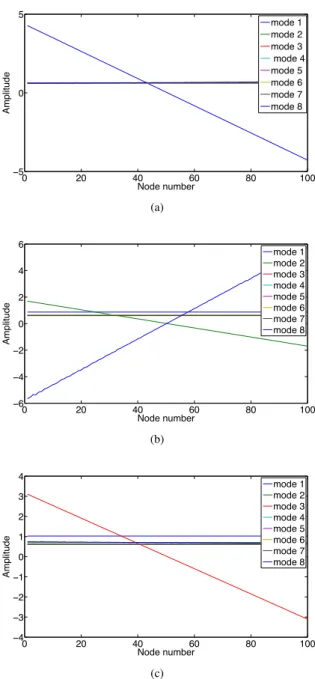
The eight first spatial modes of this PGD solution are represented in Fig.11. Modes function of initial conditions (in fact, modesGi(un) and Hi(un−1), since we are employing forward-Euler integration
Figure 10. Displacement field for the 201-th time step in the wave problem.
in the PGD loop) are represented in Figs.12and13respectively. Modes depending on the value of the external load are depicted in Fig.14.
Remark 2. Note that the discretization of the space of initial conditions must be done with an appropriate mesh. Too-coarse discretizations have led in our experience to meaningless results due to interpolation errors. For instance, in the wave propagation problem, results showing important, non-physical tractions where only compressive forces were applied have been found. It is important to estimate well the maximum amplitude that initial conditions could reach during the simulation (so as to avoid to perform extrapolations), but also a judicious choice of the meshes. Here, 100 nodes have been considered for the mesh (see Figs.12and13).
In Figs.15and16a comparison is made between the reference solution and the solution obtained with a 3-degree-of-freedom solution and one employing 8 degrees of freedom, respectively, for the parametrization of the space of initial conditions. Both employed an explicit, forward Euler, time integration.
It is noteworthy to mention that these results, for a chosen time step of t = 0.00125 s. are obtained between0.000992 and 0.001325 s. This enables the use of this technique for real-time haptic response purposes, where feedback rates between0.5−1.0 kHz are needed for a realistic touch sensation. These
results are obtained by using Matlab running on a Windows-operated HP laptop. While the complete simulation took approximately 8 seconds, the same simulation in the Abaqus software takes 16 minutes and 35 seconds (thus making it 125 times faster than the mentioned commercial software).
If, on the contrary, we employ an energy-momentum conserving scheme such as that by Bathe [8] results improve very much, and a great stability is conserved even for large integration times (10 seconds in the example depicted in Fig.17).
(a) (b) (c)
(d) (e) (f)
(g) (h)
Figure 11. Eight most important spatial modesFi(x) for the PGD solution of the wave propagation problem. Contour levels represent the value of they component of the modes.
6.2. Including non-linear strain measures
Extending the before presented technique to non-linear (hyper-)elastodynamics does not incorporate any conceptual difficulty, albeit some details deserve a comment. In [35] and [37] the authors have presented and analyzed two different approaches for the efficient linealisation of hyperelastic constitutive models in the context of quasi-static PGD models. Notably, these works present an explicit and an implicit (respectively) approach to this problem that do not imply the need to re-construct the full tangent stiffness matrix of the complete model. This constitutes an active field of research in the framework of model order reduction methods, since non-linearities usually destroy all the gains
0 20 40 60 80 100 −5 0 5 Node number Amplitude mode 1 mode 2 mode 3 mode 4 mode 5 mode 6 mode 7 mode 8 (a) 0 20 40 60 80 100 −6 −4 −2 0 2 4 6 Node number Amplitude mode 1 mode 2 mode 3 mode 4 mode 5 mode 6 mode 7 mode 8 (b) 0 20 40 60 80 100 −4 −3 −2 −1 0 1 2 3 4 Node number Amplitude mode 1 mode 2 mode 3 mode 4 mode 5 mode 6 mode 7 mode 8 (c)
Figure 12. Eight most important PGD modes Gi(un) for the wave propagation problem. Note that the function is three-dimensional, so that its components are depicted in (a), (b) and (c), respectively.
obtained in reducing the model, if tangent matrices need to be assembled.
Here, an explicit approach, similar to that in [35] has been implemented. We consider again the problem of the wave propagation in Section6.1and, without modifying the POD basis employed to
0 20 40 60 80 100 −4 −2 0 2 4 Node number Amplitude mode 1 mode 2 mode 3 mode 4 mode 5 mode 6 mode 7 mode 8 (a) 0 20 40 60 80 100 −15 −10 −5 0 5 10 15 Node number Amplitude mode 1 mode 2 mode 3 mode 4 mode 5 mode 6 mode 7 mode 8 (b) 0 20 40 60 80 100 −200 −100 0 100 200 Node number Amplitude mode 1 mode 2 mode 3 mode 4 mode 5 mode 6 mode 7 mode 8 (c)
Figure 13. Eight most important PGD modes Hi(un−1) for the wave propagation problem. Note that the function is three-dimensional, so that its components are depicted in (a), (b) and (c), respectively.
parameterize the space of initial conditions, nor any of the data of the problem, consider a Kirchhoff-Saint Venant constitutive equation for the block. We are thus considering a linear and a non-linear term
0 2 4 6 8 10 12 14 −15 −10 −5 0 5 10 15 Node Amplitude mode 1 mode 2 mode 3 mode 4 mode 5 mode 6 mode 7 mode 8
Figure 14. Eight most important PGD modes Ji(h0) for the wave propagation problem.
8.8 9 9.2 9.4 9.6 −15 −10 −5 0 x 10−5 Time [s] Amplitude [m] HHT, point A HHT, point B PGD, point A PGD, point B
Figure 15. Wave propagation problem. Solution obtained with a three-degree-of-freedom parametrization of the space of initial conditions.
for the Green-Lagrange strain tensor, E, in the form
E =1 2(F
TF − 1) = γ
l(u) + γnl(u, u), where F = ∇u + I is the gradient of deformation tensor and
γl(u) = 1 2(∇(u T) + ∇(u)), (7a) γnl(u, u) = 1 2∇(u T)∇(u). (7b)
8.8 9 9.2 9.4 9.6 9.8 10 −20 −10 0 x 10−5 Time [s] Amplitude [m] HHT, point A HHT, point B PGD, point A PGD, point B
Figure 16. Wave propagation problem. Solution obtained with an eight-degree-of-freedom parametrization of the space of initial conditions and an explicit integration in time.
8 8.5 9 9.5 10 −20 −10 0 x 10−5 Time [s] Amplitude [m] HHT, point A HHT, point B PGD, point A PGD, point B
Figure 17. Wave propagation problem. Solution obtained with an eight-degree-of-freedom parametrization of the space of initial conditions and employing the energy momentum conserving scheme by Bathe [8].
the second Piola-Kirchhoff stress tensor S can thus be obtained by
S = ∂Ψ ∂E,
that is a symmetric tensor and is related to the first Piola-Kirchhoff stress tensor, P , by P = F S. The Kirchhoff-Saint Venant model is characterized by the energy function given by
Ψ = λ 2(tr(E))
where λ and µ are Lame’s constants. The second Piola-Kirchhoff stress tensor can be obtained by
S = ∂Ψ(E)
∂E = C : E, in which C is the fourth-order constitutive (elastic) tensor.
Although it is very well known that Kirchhoff-Saint Venant model shows instabilities in compression, it provides with a very neat formulation to compare with the linear, small strains case. In Fig.18 a comparison is made between the already obtained (via HHT time integration scheme) reference, linear solution and the one considering non-linear strain measures (the so-called Kirchhoff-Saint Venant already described). As expected, non-linear strains, when considering all the remaining parameters of the problem unchanged, only provides with some bigger displacements in the solution, but an overall similar behavior of the block. Considering hyperelastic models does not imply any further delay in the response feedback given by the method here presented, since the number of on-line operations is exactly the same as for the case of linear elastic models. Of course, the off-line part of the method is somewhat more involved, but it is solved only once and stored, as repeatedly mentioned.
8.8 9 9.2 9.4 9.6 9.8 10 −20 −10 0 x 10−5 Time [s] Amplitude [m] HHT, point A HHT, point B K−SV, point A K−SV, point B
Figure 18. Wave propagation problem. Comparison of the (linear elastic) HHT reference solution with the Kirchhoff-Saint Venant one. Note that the inclusion of non-linear strain measures induces higher displacements, as expected, but an overall similar response in the problem. Solution obtained with one only mode in the POD
basis of the space of initial conditions.
6.3. Palpation of a liver
As mentioned before, computational surgery is one of the fields where real-time requirements are more astringent [13] [1]. Surgery planning provides results corresponding to large periods after the operation in a reasonable amount of time so as to allow the surgeon to take decisions in the operation room. But, notably, minimally invasive surgery simulation and training systems, equipped with haptic (force feedback) devices require us to provide responses at kHz rates.
The liver is the biggest gland in the human body, after the skin. As in [37], liver geometry has been obtained from the SOFA project [2] and post-processed in order to obtain a mesh composed by 2853 nodes and 10519 tetrahedra, whose geometry is shown in Fig.19. The anterior surface of the liver
Figure 19. Geometry of the finite element model for the liver.
is considered free, while the posterior one was assumed to be supported over different organs (it is connected to the diaphragm by the coronary ligament, for instance). The inferior vena cava travels along the posterior surface, and the liver is frequently assumed clamped a that location. Although the assumed boundary conditions are not strictly correct from a physiological point of view, our main interest is to show that the model can be solved under real-time constraints with reasonable accuracy. Here, the human liver is considered, for simplicity, as a linear elastic material withE = 0.17 MPa and ν = 0.48 [14].
Simulating a palpation, a ramp load of5 N is applied at a particular point of the liver surface during a period of0.25 seconds, and then released during other 0.25 seconds. The liver is then left vibrating free. Even if the liver tissue is well-known to posses some kind of viscoelastic properties, these have been neglected. The purpose of this example is not to obtain an extremely realistic simulation from a physiological point of view, but to show the performance of the technique. In particular, the influence of the number of modes chosen to parametrize the space of initial conditions on the long-term behaviour of the solution. To this end, a reference solution has been computed by employing an HHT time integrator and standard finite elements. POD modes have been extracted from this reference solution to construct the basis for the combined PGD-POD integrator. Other approaches, such as non-linear manifold learning [30] could also be employed and most likely would improve these results, but for the time being POD is considered as a suitable method to construct the basis.
It can be noticed that, in the idealized situation of absence of any type of damping, after the load release, the liver continues vibrating indefinitely. A PGD-POD solution has been computed by employing 1, 3 and 7 modes in the basis of the space of initial conditions. It can be noticed, from Fig.
20that increasing the number of modes, as expected, provides converging results towards the reference solution. In fact, it can be noticed how the reduction in the number of degrees of freedom, very much like in classical model order reduction, eliminates high frequencies from the solution (those with the lowest content in energy) and therefore oscillations around the reference solution can be observed. The richer the basis is, the smaller the amplitude of these oscillations and the smaller their period.
0 0.5 1 1.5 2 −0.4 −0.35 −0.3 −0.25 −0.2 −0.15 −0.1 −0.05 0 0.05 Time [s] Displacement [cm] 1 mode 3 modes 7 modes Reference 1 1.02 1.04 1.06 1.08 1.1 −0.01 0 0.01
Figure 20. Response of the liver for a peak load. Reference (FE) results, and PGD results with basis composed by 1, 3 and 7 modes.
7. Conclusions
In this paper a combined PGD-POD technique has been presented for the solution of solid dynamics problems. By formulating the problem as a parametric one, where initial conditions are the parameters, the proposed method is able to generate a sort of “black-box” integrator that takes displacement values at previous time steps as inputs and gives the solution for the current one. Within this black box any time integrator can be used. The technique here presented is aimed at solving the parametric problem, not at proposing new integrators.
This appealing approach presents, however, some difficulties. One is the enormous amount of degrees of freedom generated if every nodal displacement representing initial conditions is taken as a parameter of the formulation. To this end, an optimal bests, from the POD point of view, is used by utilizing results of similar problems computed off-line. But even then a parametric problem should be solved that may involve tens of parameters. To overcome the curse of dimensionality provoked by this fact, a PGD approach has been employed.
Thus, by computing off-line a general solution (very much like the spirit of a response surface or meta-model, but computed without the need for prior computer experiments) a kind of computational vademecum is obtained that can be emptied on-line at extremely high feedback rates, on the order of one kHz.
Previous works of the authors have shown how to include within this general formulation parameters such as load position, value and orientation, and how to efficiently solve non-linearities arising from material constitutive equations [35] [37]. This work on the dynamics of the problem somehow closes one fundamental aspect: that related with the interactivity of the simulation with the user, thus
configuring a true dynamic data driven application system (DDDAS).
Some fundamental aspects remain open, however. For instance, within the computational surgery applications, surgery cutting is a fundamental aspect to achieve realism in the simulation. Within this framework, an algorithm should be developed able to predict the response of the organ to a surgical cut placed at any point of the model and with arbitrary length. This constitutes one of our current efforts of research.
REFERENCES
1. I. Alfaro, D. Gonzalez, F. Bordeu, A. Leygue, A. Ammar, E. Cueto, and F. Chinesta. Real-time in silico experiments on gene regulatory networks and surgery simulation on handheld devices. Journal of Computational Surgery, in press, 2013. 2. J´er´emie Allard, St´ephane Cotin, Franc¸ois Faure, Pierre-Jean Bensoussan, Franc¸ois Poyer, Christian Duriez, Herv´e Delingette, and Laurent Grisoni. SOFA an Open Source Framework for Medical Simulation. In Medicine Meets Virtual Reality (MMVR’15), Long Beach, USA, February 2007.
3. A. Ammar, F. Chinesta, P. Diez, and A. Huerta. An error estimator for separated representations of highly multidimensional models. Computer Methods in Applied Mechanics and Engineering, 199(25-28):1872 – 1880, 2010.
4. A. Ammar, B. Mokdad, F. Chinesta, , and R. Keunings. A new family of solvers for some classes of multidimensional partial differential equations encountered in kinetic theory modeling of complex fluids. part ii: transient simulation using space-time separated representations. J. Non-Newtonian Fluid Mech., 144:98–121, 2007.
5. A. Ammar, B. Mokdad, F. Chinesta, and R. Keunings. A new family of solvers for some classes of multidimensional partial differential equations encountered in kinetic theory modeling of complex fluids. J. Non-Newtonian Fluid Mech., 139:153–176, 2006.
6. Jernej Barbiˇc and Doug James. Time-critical distributed contact for 6-DoF haptic rendering of adaptively sampled reduced deformable models. In Metaxas, D and Popovic, J, editor, SYMPOSIUM ON COMPUTER ANIMATION 2007: ACM SIGGRAPH/ EUROGRAPHICS SYMPOSIUM PROCEEDINGS, pages 171–180, 1515 BROADWAY, NEW YORK, NY 10036-9998 USA, 2007. ACM SIGGRAPH; Eurog Assoc, ASSOC COMPUTING MACHINERY. Symposium on Computer Animation, San Diego, CA, AUG 03-04, 2007.
7. Jernej Barbiˇc and Doug L. James. Real-time subspace integration for St. Venant-Kirchhoff deformable models. ACM Transactions on Graphics (SIGGRAPH 2005), 24(3):982–990, August 2005.
8. K. J. Bathe. Conserving energy and momentum in nonlinear dynamics: A simple implicit time integration scheme. Computers and Structures, 85:437–445, 2007.
9. L. Boucinha, A. Gravouil, and A. Ammar. Space-time proper generalized decompositions for the resolution of transient elastodynamic models. Computer Methods in Applied Mechanics and Engineering, 255(0):67 – 88, 2013.
10. F. Chinesta, A. Ammar, and E. Cueto. Recent advances in the use of the Proper Generalized Decomposition for solving multidimensional models. Archives of Computational Methods in Engineering, 17(4):327–350, 2010.
11. F. Chinesta, A. Leygue, F. Bordeu, J.V. Aguado, E. Cueto, D. Gonzalez, I. Alfaro, A. Ammar, and A. Huerta. PGD-Based Computational Vademecum for Efficient Design, Optimization and Control. Archives of Computational Methods in Engineering, 20(1):31–59, 2013.
12. Francisco Chinesta, Pierre Ladeveze, and Elias Cueto. A short review on model order reduction based on proper generalized decomposition. Archives of Computational Methods in Engineering, 18:395–404, 2011.
13. El´ıas Cueto and Francisco Chinesta. Real time simulation for computational surgery. a review. Advanced Modeling and Simulation in Engineering Sciences, submitted, 2013.
14. H. Delingette and N. Ayache. Soft tissue modeling for surgery simulation. In N. Ayache, editor, Computational Models for the Human Body, Handbook of Numerical Analysis (Ph. Ciarlet, Ed.), pages 453–550. Elsevier, 2004.
15. D. Gonzalez, F. Masson, F. Poulhaon, E. Cueto, and F. Chinesta. Proper generalized decomposition based dynamic data driven inverse identification. Mathematics and Computers in Simulation, 82:1677–1695, 2012.
16. D. Gonz´alez, A. Ammar, F. Chinesta, and E. Cueto. Recent advances on the use of separated representations. International Journal for Numerical Methods in Engineering, 81(5), 2010.
17. Ch. Heyberger, P.-A. Boucard, and D. Neron. A rational strategy for the resolution of parametrized problems in the {PGD} framework. Computer Methods in Applied Mechanics and Engineering, 259(0):40 – 49, 2013.
18. H. M. Hilber, T. J. R. Hughes, and R. L. Taylor. Improved numerical dissipation for time integration algorithms in structural dynamics. Earthquake Engineering and Structural Dynamics, 5:283–292, 1977.
19. S. R. Idelsohn and R. Cardona. A reduction method for nonlinear structural dynamics analysis. Computer Methods in Applied Mechanics and Engineering, 49:253–279, 1985.
20. K. Karhunen. Uber lineare methoden in der wahrscheinlichkeitsrechnung. Ann. Acad. Sci. Fennicae, ser. Al. Math. Phys., 37, 1946.
21. P. Krysl, S. Lall, and J.E. Marsden. Dimensional model reduction in non-linear finite element dynamics of solids and structures. Int. J. Numer. Meth. in Engng., 51:479–504, 2001.
22. P. Ladeveze. Nonlinear Computational Structural Mechanics. Springer, N.Y., 1999.
23. P. Ladeveze, J.-C. Passieux, and D. Neron. The latin multiscale computational method and the proper generalized decomposition. Computer Methods in Applied Mechanics and Engineering, 199(21-22):1287 – 1296, 2010.
24. Pierre Ladeveze and Ludovic Chamoin. On the verification of model reduction methods based on the proper generalized decomposition. Computer Methods in Applied Mechanics and Engineering, 200(23-24):2032–2047, 2011.
25. Sanjay Lall, Petr Krysl, and Jerrold E Marsden. Structure-preserving model reduction for mechanical systems. Physica D: Nonlinear Phenomena, 184(1-4):304–318, 2003.
26. R. B. Laughlin and David Pines. The theory of everything. Proceedings of the National Academy of Sciences, 97(1):28–31, 2000.
27. M. M. Lo`eve. Probability theory. The University Series in Higher Mathematics, 3rd ed. Van Nostrand, Princeton, NJ, 1963.
28. E. N. Lorenz. Empirical Orthogonal Functions and Statistical Weather Prediction. MIT, Departement of Meteorology, Scientific Report Number 1, Statistical Forecasting Project, 1956.
29. M. Meyer and H. G. Matthies. Efficient model reduction in non-linear dynamics using the Karhunen-Lo`eve expansion and dual-weighted-residual methods. Computational Mechanics, 31(1-2):179–191, 2003.
30. Daniel Mill´an and Marino Arroyo. Nonlinear manifold learning for model reduction in finite elastodynamics. Computer Methods in Applied Mechanics and Engineering, 261-262(0):118 – 131, 2013.
31. J. P. Moitinho de Almeida. A basis for bounding the errors of proper generalised decomposition solutions in solid mechanics. International Journal for Numerical Methods in Engineering, 94(10):961–984, 2013.
32. R.E. Nickell. Nonlinear dynamics by mode superposition. Computer Methods in Applied Mechanics and Engineering, 7(1):107 – 129, 1976.
33. S. Niroomandi, I. Alfaro, E. Cueto, and F. Chinesta. Real-time deformable models of non-linear tissues by model reduction techniques. Computer Methods and Programs in Biomedicine, 91(3):223 – 231, 2008.
34. S. Niroomandi, I. Alfaro, E. Cueto, and F. Chinesta. Accounting for large deformations in real-time simulations of soft tissues based on reduced-order models. Computer Methods and Programs in Biomedicine, 105(1):1–12, 2012.
35. S. Niroomandi, D. Gonz´alez, I. Alfaro, F. Bordeu, A. Leygue, E. Cueto, and F. Chinesta. Real-time simulation of biological soft tissues: a pgd approach. International Journal for Numerical Methods in Biomedical Engineering, 29(5):586–600, 2013.
36. Siamak Niroomandi, Iciar Alfaro, Elias Cueto, and Francisco Chinesta. Model order reduction for hyperelastic materials. International Journal for Numerical Methods in Engineering, 81(9):1180–1206, 2010.
37. Siamak Niroomandi, Ic´ıar Alfaro, David Gonz´alez, El´ıas Cueto, and Francisco Chinesta. Model order reduction in hyperelasticity: a proper generalized decomposition approach. International Journal for Numerical Methods in Engineering, 96(3):129–149, 2013.
38. A. NOOR and J. PETERS. Reduced basis technique for nonlinear analysis of structures. American Institute of Aeronautics and Astronautics, 2013/10/16 1979.
39. Anthony Nouy. A priori model reduction through Proper Generalized Decomposition for solving time-dependent partial differential equations. Computer Methods in Applied Mechanics and Engineering, 199(23-24):1603–1626, 2010. 40. H. M. Park and D. H. Cho. The use of the Karhunen-Lo`eve decomposition for the modeling of distributed parameter
systems. Chemical Engineering Science, 51(1):81–98, 1996.
41. A. Radermacher and S. Reese. Proper orthogonal decomposition-based model reduction for nonlinear biomechanical analysis. International Journal of Materials Engineering Innovation, 4(4):149–165, 2013.
42. L. Sirovich. Turbulence and the dynamics of coherent structures part I: coherent structures. Quaterly of applied mathematics, XLV:561–571, 1987.
43. Z.A. Taylor, M. Cheng, and S. Ourselin. High-speed nonlinear finite element analysis for surgical simulation using graphics processing units. Medical Imaging, IEEE Transactions on, 27(5):650 –663, may 2008.
44. Z.A. Taylor, S. Crozier, and S. Ourselin. A reduced order explicit dynamic finite element algorithm for surgical simulation. Medical Imaging, IEEE Transactions on, 30(9):1713 –1721, sept. 2011.
45. Z.A. Taylor, S. Ourselin, and S. Crozier. A reduced order finite element algorithm for surgical simulation. In Engineering in Medicine and Biology Society (EMBC), 2010 Annual International Conference of the IEEE, pages 239 –242, 31 2010-sept. 4 2010.
46. Otto von Estorff and Christian Hagen. Iterative coupling of fem and bem in 3d transient elastodynamics. Engineering Analysis with Boundary Elements, 30(7):611 – 622, 2006.


![Figure 6. Comparison of the results of the beam in Section. 4.3. Explicit vs. Energy-Momentum conserving integration proposed in [8].](https://thumb-eu.123doks.com/thumbv2/123doknet/8274669.278627/12.892.247.612.200.454/figure-comparison-section-explicit-momentum-conserving-integration-proposed.webp)