HAL Id: hal-01816528
https://hal.archives-ouvertes.fr/hal-01816528
Submitted on 15 Jun 2018
HAL is a multi-disciplinary open access
archive for the deposit and dissemination of
sci-entific research documents, whether they are
pub-lished or not. The documents may come from
teaching and research institutions in France or
L’archive ouverte pluridisciplinaire HAL, est
destinée au dépôt et à la diffusion de documents
scientifiques de niveau recherche, publiés ou non,
émanant des établissements d’enseignement et de
recherche français ou étrangers, des laboratoires
non-stationary determinantal point processes
Frédéric Lavancier, Arnaud Poinas, Rasmus Waagepetersen
To cite this version:
Frédéric Lavancier, Arnaud Poinas, Rasmus Waagepetersen. Adaptive estimating function inference
for non-stationary determinantal point processes. Scandinavian Journal of Statistics, Wiley, 2021, 48
(1), pp.87-107. �10.1111/sjos.12440�. �hal-01816528�
Adaptive estimating function inference for
non-stationary determinantal point processes
FR ´ED ´ERIC LAVANCIER1,* ARNAUD POINAS2,** RASMUS WAAGEPETERSEN3,†
1
Laboratoire de Math´ematiques Jean Leray – BP 92208 – 2, Rue de la Houssini`ere – F-44322 Nantes Cedex 03 – France. Inria, Centre Rennes Bretagne Atlantique, France.
E-mail:*[email protected]
2IRMAR – Campus de Beaulieu - Bat. 22/23 – 263 avenue du G´en´eral Leclerc – 35042 Rennes – France
E-mail:**
3
Department of Mathematical Sciences – Aalborg University - Fredrik Bajersvej 7G – DK-9220 Aalborg – Denmark
E-mail:†[email protected]
Estimating function inference is indispensable for many common point process models where the joint intensities are tractable while the likelihood function is not. In this paper we es-tablish asymptotic normality of estimating function estimators in a very general setting of non-stationary point processes. We then adapt this result to the case of non-stationary determi-nantal point processes which are an important class of models for repulsive point patterns. In practice often first and second order estimating functions are used. For the latter it is common practice to omit contributions for pairs of points separated by a distance larger than some trun-cation distance which is usually specified in an ad hoc manner. We suggest instead a data-driven approach where the truncation distance is adapted automatically to the point process being fit-ted and where the approach integrates seamlessly with our asymptotic framework. The good performance of the adaptive approach is illustrated via simulation studies for non-stationary determinantal point processes.
Keywords: asymptotic normality, determinantal point processes, estimating functions, joint
in-tensities, non-stationary, repulsive.
1. Introduction
A common feature of spatial point process models (except for the Poisson process case) is that the likelihood function is not available in a simple form. Numerical approximations of the likelihood function are available [see e.g. 12,13, for reviews] but the approaches are often computationally demanding and the distributional properties of the approxi-mate maximum likelihood estiapproxi-mates may be difficult to assess. Therefore much work has focused on establishing computationally simple estimation methods that do not require knowledge of the likelihood function.
In this paper we focus on estimation methods for point processes which have known joint intensity functions. This includes many cases of Cox and cluster point process mod-els [12,7,1] as well as determinantal point processes [11,17,16,8]. These classes of models are quite different since realizations of Cox and cluster point processes are aggregated while determinantal point processes produce regular point pattern realizations.
Knowledge of an nth order joint intensity enables the use of the so-called Campbell formulae for computing expectations of statistics given by random sums indexed by n-tuples of distinct points in a point process. Unbiased estimating functions can then be constructed from such statistics by subtracting their expectations. So far mainly the cases of first and second order joint intensities have been considered where the first order joint intensity is simply the intensity function. However, consideration of higher order estimating functions may be worthwhile to obtain more precise estimators or to identify parameters in complex point process models.
Theoretical results have been established in a variety of special cases of first and second order estimating functions for Cox and cluster processes [15,5,22,6,23] and for the closely related Palm likelihood estimators [20,18,19]. The common general structure of the estimating functions on the other hand calls for a general theoretical set-up which is the first contribution of this paper. Our set-up also covers third or higher order estimating functions and combinations of such estimating functions.
The literature on statistical inference for determinantal point processes is quite limited with theoretical results so far only available in case of minimum contrast estimation for stationary determinantal point processes [3]. Based on the general set-up our second main contribution is to provide a detailed theoretical study of estimating function estimators for general non-stationary determinantal point processes.
Specializing to second-order estimating functions, a common approach [5, 20] is to restrict the random sum to pairs of R-close points for some user-specified R ą 0. This may lead to faster computation and improved statistical efficiency. The properties of the resulting estimators depend strongly on R but only ad hoc guidance is available for the choice of R. Moreover, it is difficult to account for ad hoc choices of R when establishing theoretical results. Our third contribution is a simple intuitively appealing adaptive choice of R which leads to a theoretically tractable estimation procedure and we demonstrate its usefulness in simulation studies for determinantal point processes as well as an example of a cluster process.
2. Estimating functions based on joint intensities
A point process X on Rd, d ě 1, is a locally finite random subset of Rd. For B Ď Rd, we let N pBq denote the random number of points in X X B. That X is locally finite means that N pBq is finite almost surely whenever B is bounded. The so-called joint intensities of a point process are described in Section2.1. In this paper we mainly focus on determinantal point processes, detailed in Section 3. A prominent feature of determinantal point processes is that they have known joint intensity functions of any order.
2.1. Joint intensity functions and Campbell formulae
For integer n ě 1, the joint intensity ρpnqof nth order is defined byE ‰ ÿ u1,...,unPX 1u1PB1,...,unPBn “ ż ˆn i“1Bi ρpnqpu1, . . . , unqdu1¨ ¨ ¨ dun (1)
for Borel sets Bi Ď Rd, i “ 1, . . . , n, assuming that the left hand side is absolutely
continuous with respect to Lebesgue measure on Rd. The ‰ over the summation sign means that the sum is over pairwise distinct points in X. Of special interest are the cases n “ 1 and n “ 2 where the intensity function ρ “ ρp1q and the second order joint
intensity ρp2qdetermine the first and second order moments of the count variables N pBq,
B Ď Rd. The pair correlation function gpu, vq is defined as
gpu, vq “ ρ
p2qpu, vq ρpuqρpvq
whenever ρpuqρpvq ą 0 (otherwise we define gpu, vq “ 0). The product ρpuqgpu, vq can be interpreted as the intensity of X at u given that v P X. Hence gpu, vq ą 1 (ă 1) means that presence of a point at v increases (decreases) the likeliness of observing yet another point at u. The Campbell formula
E ‰ ÿ u1,...,unPX f pu1, . . . , unq “ ż f pu1, . . . , unqρpnqpu1, . . . , unqdu1¨ ¨ ¨ dun
follows immediately from the definition of ρpnqfor any non-negative function f : pRd
qn Ñ r0, 8r.
2.2. A general asymptotic result for estimating functions
Consider a parametric family of distributions tPθ: θ P Θu of point processes on Rd, where
Θ is a subset of Rp
. We assume a realization of the point process X with distribution Pθ˚,
θ˚P IntpΘq, is observed on a window W
nĂ Rd. We estimate the unknown parameter θ˚
by the solution ˆθn of enpθq “ 0 where
enpθq “ ¨ ˚ ˚ ˝ ř‰ u1,¨¨¨ ,uq1PXXWnf1pu1, ¨ ¨ ¨ , uq1; θq ´ ş Wnq1f1pu; θqρ pq1qpu; θqdu .. . ř‰ u1,¨¨¨ ,uqlPXXWnflpu1, ¨ ¨ ¨ , uql; θq ´ ş Wnqlflpu; θqρ pqlqpu; θqdu ˛ ‹ ‹ ‚
for l given functions fi: pRdqqiˆ Θ Ñ Rki such that
ř
iki“ p.
A basic assumption for the following theorem (verified in AppendixA) is that a central limit theorem is available for enpθ˚q (assumption (X3)). In addition to this, a number of
technical assumptions (F1) through (F3) (or (F3’)), (X1) and (X2) regarding existence and differentiability of joint intensities as well as differentiability of the fi are needed.
All the conditions are listed in AppendixA.
Theorem 2.1. Under Assumptions (F1) through (F3) (or (F3’)), (X1) and (X2), with
a probability tending to one as n Ñ 8, there exists a sequence of roots ˆθn of the estimating
equations enpθq “ 0 for which
ˆ
θnÝÑ θP ˚.
Moreover, if (X3) holds true, then
|Wn|Σ´1{2n Hnpθ˚qpˆθn´ θ˚q
L
ÝÑ N p0, Ipq.
where Σn“ Varpenpθ˚qq, Hnpθ˚q is defined in (F3), and Ip is the p ˆ p identity matrix.
2.3. Second order estimating functions
Referring to the previous section, much attention has been devoted to instances of the case l “ 1, q1“ 2 and k1“ p. In this case we obtain a second-order estimating function
of the form enpθq “ ‰ ÿ u,vPXXWn f pu, v; θq ´ ż W2 n f pu, v; θqρp2q pu, v; θqdudv. (2)
[5] noted that for computational and statistical efficiency it may be advantageous to use only close pairs of points rather than all pairs of points. Thus in (2) it is common practice to introduce an indicator1}u´v}ďRfor some constant 0 ă R or choose f so that
f pu, vq “ 0 whenever }u ´ v} ą R. We discuss a method for choosing R in Section2.4.
The general form (2) includes e.g. the score functions of second-order composite likeli-hood [5,22] and Palm likelihood functions [20,18,19] as well as score functions of mini-mum contrast object functions based on non-parametric estimates of summary statistics as the K or the pair correlation function. For the second-order composite likelihood of [5], f pu, v; θq “ ∇θρ p2qpu, v; θq ρp2qpu, v; θq ´ ş W2∇θρp2qpu, v; θqdudv ş W2ρp2qpu, v; θqdudv while f pu, v; θq “ ∇θρ p2qpu, v; θq ρp2qpu, v; θq
for the second-order composite likelihood proposed in [22]. The score of the Palm likeli-hood as generalized to the inhomogeneous case in [19] is obtained with
f pu, v; θq “ ∇θρ p2q pu,v;θq ρpu;θq ρp2qpu, v; θq{ρpu; θq´ 1 N pW q ´ 1 ż W ∇θ ˆ ρp2qpu, w; θq ρpu; θq ˙ dw.
[19] also regarded the second-order composite likelihood proposed in [22] as a general-ization of the stationary case Palm likelihood but the interpretation as a second-order composite likelihood given in [22] is more straightforward.
Considering a class of estimating functions of the form (2) a natural question is what is the optimal choice of f ? [4] provides a solution to this problem where an approximation of the optimal f is obtained by solving numerically a certain integral equation. This yields a statistically optimal estimation procedure but is computationally demanding and requires specification of third and fourth order joint intensities. When computational speed and ease of use is an issue, there is still scope for simpler methods. Moreover, given several (simple) estimation methods, it is possible to combine them adaptively in order to build a final estimator that achieves better properties than each initial estimator, see [9,10].
2.4. Adaptive version
Consider second-order composite likelihood using only R close pairs. The weight function
f is then of the form
fRpu, v; θq “1}u´v}ďR
∇θρp2qpu, v; θq
ρp2qpu, v; θq . (3)
The performance of the parameter estimates can depend strongly on the chosen R. Sim-ulation studies such as in [19] and [4] usually compare results for several values of R corresponding to different multiples of some parameter associated with ‘range of corre-lation’. For a cluster process this parameter could e.g. be the standard deviation of the distribution for dispersal of offspring around parents. For a determinantal point process the parameter would typically be a correlation scale parameter in the kernel of the de-terminantal point process, see Section3. In practice these parameters are not known and among the quantities that need to be estimated. [5] suggested to choose an R that min-imizes a goodness of fit criterion for the fitted point process model while [23] suggested to choose R by inspection of a non-parametric estimate of the pair correlation function. Both approaches imply extra work and ad hoc decisions by the user and it becomes very complex to determine the statistical properties of the resulting parameter estimates.
A typical behaviour of many pair correlation functions is that gpu, v; θq converges to a limiting value of 1 when }u ´ v} increases and |gpu, v; θq ´ 1| ď |gpu, u; θq ´ 1| where the upper bound does not depend on u. If gpu, v; θq “ 1 for }u ´ v} ą r0 then counts of
points are uncorrelated when they are observed in regions separated by a distance of r0.
Following the idea that R should depend on some range property of the point process we therefore suggest to replace the constraint }u ´ v} ă R in (3) by the constraint
|gpu, v; θq ´ 1| |gpu, u; θq ´ 1| ą ε,
for a small ε. If e.g. ε “ 1% this means that we only consider pairs of points pu, vq so that the difference between gpu, v; θq and the limiting value 1 is within 1% of the maximal
value |gpu, u; θq ´ 1|. Note that this choice of pairs of points is adaptive in that it depends on θ.
We then modify the function fR to be
fadappu, v; θq “ w ˆ εgpu, u; θq ´ 1 gpu, v; θq ´ 1 ˙ ∇θρp2qpu, v; θq ρp2qpu, v; θq (4)
where w is some weight function of bounded support r´1, 1s. Later on, when establishing asymptotic results, we will also assume that w is differentiable. A common example of admissible weight function is wprq “ e1{pr2´1q for ´1 ď r ď 1, while wprq “ 0 otherwise.
The user needs to specify a value of ε but in contrast to the original tuning parameter
R, ε has an intuitive meaning independent of the underlying point process. We choose
ε “ 1%. In the simulation study in Section 4.1 we also consider ε “ 5% in order to
investigate the sensitivity to the choice of ε.
3. Asymptotic results for determinantal point
processes
A point process X is a determinantal point process (DPP for short) with kernel K : Rdˆ RdÑ R if for all n ě 1, the joint intensity ρpnqexists and is of the form
ρpnq
pu1, . . . , unq “ detrKspu1, . . . , unq
for all tu1, . . . , unu Ă Rd, where rKspu1, . . . , unq is the matrix with entries Kpui, ujq.
The intensity function is thus ρpuq “ Kpu, uq, u P Rd. If a determinantal point process with kernel K exists it is unique. General conditions for existence are presented in [8]. In particular, if K admits the form
Kpu, vq “aρpuqρpvqCpu ´ vq
for a function C : Rd
Ñ R with Cp0q “ 1, then a sufficient condition for existence of a DPP with kernel K is that ρ is bounded and that C is a square integrable continuous covariance function with spectral density bounded by 1{}ρ}8. The normalization Cp0q “
1 ensures that ρ is the intensity of the DPP.
We now consider a parametric family of DPPs on Rd with kernels K
θ where θ P Θ
and Θ Ď Rp [see 8, 2, for examples of such families]. Henceforth, we assume that K θ is
symmetric and the DPP with kernel Kθ exists for all θ P Θ.
[8] provide an expression for the likelihood of a DPP on a bounded window and dis-cuss likelihood based inference for stationary DPPs. However, the expression depends on a spectral representation of K which is rarely known in practice and must be ap-proximated numerically. Letting n denote the number of observed points, the likelihood further requires the computation of an n ˆ n dense matrix which can be time consuming for large n. As an alternative, [2] consider minimum contrast estimation based on the pair correlation function or Ripley’s K-function, but only for stationary DPPs. In the
following, we consider general non-stationary DPPs and the estimator ˆθn obtained by
solving enpθq “ 0 where en is given by (2).
We establish in Section3.1 using Theorem2.1the asymptotic properties of the esti-mate ˆθn where en is given by (2) for a wide class of test functions f . In Section3.2, we
focus on a particular case of the DPP model, where the parameter θ “ pβ, ψq can be separated into a parameter β only appearing in the intensity function and a parameter ψ only appearing in the pair correlation function. Following [23], it is natural to consider a two-step estimation procedure where in a first step β is estimated by a Poisson likelihood score estimating function, and in a second step the remaining parameter ψ is estimated by a second order estimating function as in (2), where β is replaced by ˆβnobtained in the
first step. The asymptotic properties of this two-step procedure again follow as a special case of Theorem2.1.
3.1. Second order estimating functions for DPPs
We assume a realization of a DPP X with kernel Kθ˚, θ˚ P IntpΘq, is observed on
a window Wn Ă Rd. We estimate the unknown parameter θ˚ by the solution ˆθn of
enpθq “ 0 where enpθq is given by (2) for a given Rp-valued function f . Therefore, we are
in a special case of the set-up in Section2.2with l “ 1, q1“ 2, k1“ p and we assume that f1“ f satisfies the assumptions (F1) through (F3) (or (F3’)) listed in AppendixA. The
condition (F1) in this case demands that θ ÞÑ f pu, v; θq is twice continuously differentiable in a neighbourhood of θ˚ and for θ in this neighbourhood, the derivatives are bounded
with respect to pu, vq uniformly in θ. Moreover, from (F2), there exists R ą 0 such that for all θ in a neighbourhood of θ˚,
f pu, v; θq “ 0 if }u ´ v} ą R. (5)
Concerning (F3) (or (F3’)), this condition controls the asymptotic behaviour of the ma-trix Hnpθq given by Hnpθq “ 1 |Wn| ż W2 n
f pu, v; θq∇θρp2qpu, v; θqTdudv,
where we recall that in this setting
ρp2qpu, v; θq “ Kθpu, uqKθpv, vq ´ Kθpu, vq2. (6)
The assumptions (F3) and (F3’) are technical and needed for the identifiability of the estimation procedure. When Hn is a symmetric matrix, assumption (F3) seems simpler
to verify than (F3’). As an important example, when f is defined as in (4), we prove in Lemmas3.2and3.3that (F3) is generally satisfied even if X is not stationary.
Finally, as shown in the proof of Theorem3.1 below, the assumptions (X1) through (X3) in Theorem 2.1become:
(D1) θ ÞÑ Kθpu, vq is twice continuously differentiable in a neighborhood of θ˚, for all
u, v P Rd. Moreover, the first and second derivative of K
θ with respect to θ are
bounded with respect to u, v P Rd uniformly in θ in a neighborhood of θ˚.
(D2) The kernel Kθ˚ satisfies, for some ε ą 0,
sup
}u´v}ąr
Kθ˚pu, vq “ opr´pd`εq{2q.
(D3) lim infnλminp|Wn|´1Σnq ą 0 where Σn:“ Varpenpθ˚qq.
(W) Dε ą 0 s.t. |BWn‘ pR ` εq| “ op|Wn|q, where B in this context denotes the boundary
of a set, R is defined in (5), and |Wn| Ñ 8, as n Ñ 8.
Let us briefly comment on these assumptions. (D1) is a standard regularity assump-tion. Condition (D2) is not restrictive since all standard parametric kernel families satisfy
sup}u´v}ąrKθpu, vq “ Opr´pd`1q{2q, including the most repulsive stationary DPP [see
8, 2]. Condition (D3) ensures that the asymptotic variance in the central limit theorem below is not degenerated. Finally, Assumption (W) makes specific the fact that Wn is
not too irregularly shaped and tends to infinity in all directions. It is for instance fulfilled if Wn is a Cartesian product of d intervals whose lengths tends to infinity.
Theorem 3.1. Under Assumptions (D1) and (D2), if assumptions (F1) through (F3)
(or (F3’)) are satisfied for f1 “ f , with a probability tending to one as n Ñ 8, there
exists a sequence of roots ˆθn of the estimating equations enpθq “ 0 for which
ˆ
θnÝÑ θP ˚.
If moreover (W) and (D3) holds true, then
|Wn|Σ´1{2n Hnpθ˚qpˆθn´ θ˚q
L
ÝÑ N p0, Ipq.
Proof. We deduce from (6) that (D1) implies (X1). Moreover, it was shown in [14] that (X2) is a consequence of (D2) and that (X3) is a consequence of (D2), (D3) and (W). Thus, we can conclude by applying Theorem (2.1) in the case l “ 1 and q1“ 2.
In the case of a stationary X and f given by (4), the following lemma shows that (F3) is satisfied under mild assumptions that are violated only in degenerate cases. For instance, if p “ 1, the main assumption boils down to ∇θρp2qp0, t; θ˚q ‰ 0 for some t ‰ 0
such that |Kθ˚ptq| ą
?
εKθ˚p0q.
Lemma 3.2. Assume (W) and (D2), suppose X is stationary and let f be as in (4).
Let h : Rd Ñ MppRq be defined by hptq “ wˆ εKθ˚p0q 2 Kθ˚ptq2 ˙ ∇θρp2qp0, t; θ˚q∇θρp2qp0, t; θ˚qT ρp2qp0, t; θ˚q .
Assume that w is positive on r0, 1r. If h is integrable at the origin and if spant∇θρp2qp0, t; θ˚q :
|Kθ˚ptq| ą
?
Proof. By definition of w and (D2), there exists R ą 0 such that hptq “ 0 when }t} ě R. By Lemma A.1, Hnpθ˚q converges towards the positive semi-definite matrix Hpθ˚q “
ş
}t}ăRhptqdt. In this case, proving (F3) is equivalent to showing that φ
THpθ˚qφ “ 0 only
if φ “ 0. For this, let A be the set of t such that |Kθ˚ptq| ą
?
εKθ˚p0q, φ P Rp and
note that since wpεKθ˚p0q2{Kθ˚ptq2q ą 0 for t P A and hptq is continuous and positive
semi-definite, φTHpθ˚qφ “ 0 ô @t P A, φT hptqφ “ 0 ô @t P A, ∇θρp2qp0, t; θ˚qTφ “ 0 ô φ P´spant∇θρp2qp0, t; θ˚q : t P Au ¯K .
By assumption spant∇θρp2qp0, t; θ˚q : t P Au “ Rp whereby φ “ 0, which concludes the
proof.
Similarly, we can show that even in the non-stationary case, condition (F3) is satis-fied for the function in (4) but under slightly stronger assumptions on ∇θρp2qpu, v; θ˚q.
Namely, we demand that all functions v ÞÑ ∇θρp2qpu, v; θ˚q are not contained in a single
hyperplane of Rp nor confined around 0. This is similar in essence to what we have
as-sumed in the previous corollary but with the need of a uniform condition with respect to u. Functions that do not satisfy these requirements are arguably degenerate.
Lemma 3.3. Assume (W), (D2) and that Kθ˚ is bounded. Let f be as in (4) and define
h : RdÑ MppRq by
hpu, vq “ wˆ εKθ˚pu, uqKθ˚pv, vq
Kθ˚pu, vq2
˙ ∇θρp2qpu, v; θ˚q∇θρp2qpu, v; θ˚qT
ρp2qpu, v; θ˚q .
Assume that w is positive on r0, 1r. If supu}hpu, .q} is integrable and if there exists µ ą 1
and δ ą 0 such that for all u P Rd
and for all unit vectors φ of Rp there exists a subset
A of tv : Kθ˚pu, vq2ą µεKθ˚pu, uqKθ˚pv, vqu of positive Lebesgue measure |A| ą 0 and
satisfying
@v P A, |φT∇θρp2qpu, v; θ˚q| ą δ
then (F3) is satisfied.
Proof. By definition of w, (D2) and the fact that Kθ˚ is bounded, there exists R ą 0
such that hpu, vq “ 0 when }v ´ u} ě R. The integral in (F3) writes
Hnpθ˚q “
ż
W2
n
hpu, vq1}u´v}ďRdvdu “
ż
WaR
n
ż
Wn
hpu, vq1}u´v}ďRdvdu ` εn
where εn“ ż WnzWnaR ż Wn
By (W), we have }εn} |Wn| ď |WnzW aR n | |Wn| ż }v´u}ăR sup uPRd }hpu, vq}dv ď |BWn‘ R| |Wn| ż }v´u}ăR sup uPRd }hpu, vq}dv Ñ 0,
and for all φ,
φT
ˆż
WnaR
ż
Wn
hpu, vq1}u´v}ďRdudv
˙ φ “ ż WnaR ˜ ż }u´v}ďR φThpu, vqφdv ¸ du.
By our assumption on ∇θρp2q, there exists a set A of positive Lebesgue measure such
that
@v P A, ∇θρp2qpu, v; θ˚q P spantφu X Bp0, δqC
and wˆ εKθ˚pu, uqKθ˚pv, vq
Kθ˚pu, vq2 ˙ ą inf xPr0,1{µswpxq. Hence for }φ} “ 1, 1 |Wn| φT ˆż WnaR ż Wn
hpu, vq1}u´v}ďRdudv
˙ φ ě infxPr0,1{µswpxq |Wn|}ρp2qp., .; θ˚q}8 ż WnaR ˆż A |φT∇θρp2qpu, v; θ˚q|2dv ˙ du ě|W aR n ||A|δ2infxPr0,1{µswpxq |Wn|}ρp2qp., .; θ˚q}8 Ñ|A|δ 2inf xPr0,1{µswpxq }ρp2qp., .; θ˚q} 8 ą 0
and since the limit does not depend on φ, (F3) is satisfied.
3.2. Two-step estimation for a separable parameter
We consider a family of kernelsKθpu, vq “
a
ρpu; βqCpu, v; ψqaρpv; βq,
where θ :“ pβT, ψTqT P Θ Ă Rp`q with β P Rp and ψ P Rq, ρp.; βq are non-negative functions, and Cp¨, ¨; ψq are correlation functions, in particular Cpu, u; ψq “ 1 for any ψ. Note that in this case the DPP with kernel Kθhas intensity ρp.; βq and its pair correlation
function is gpu, v; ψq “ 1 ´ C2
As in the preceding section, we assume a DPP X with kernel Kθ˚, θ˚ P IntpΘq, is
observed on a window Wn Ă Rd. In the spirit of [23], we estimate θ˚ in two steps. First,
β˚ is estimated as the solution ˆβ
n of snpβq “ 0 where snpβq “ ÿ uPXXWn ∇βρpu; βq ρpu; βq ´ ż Wn ∇βρpu; βqdu
is the score function for a Poisson point process. Then, we estimate ψ˚ by the solution
ˆ ψn of unpp ˆβn, ψq “ 0 where unpθq “ ‰ ÿ u,vPXXWn f pu, v; θq ´ ż W2 n f pu, v; θqρp2q pu, v; θqdudv
for a given Rq-valued function f and where ρp2qpu, v; θq “ ρp2qpu, v; β, ψq “ ρpu; βqρpv; βqp1´ C2pu, v; ψqq in this case. Here and in the following for convenience of notation e.g. identify
unpβ, ψq with unpθq when θ “ pβT, ψTqT.
This two-step procedure is a particular estimating equation procedure, since ˆθn :“
p ˆβT
n, ˆψTnqT is obtained as the solution of enpθq “ 0 where enpθq “ psnpβqT, unpβ, ψqTqT.
Thus, this is a particular case of the setting in Section2.2where l “ 2, q1“ 1, q2 “ 2,
f1“ ∇βρpu; βq{ρpu; βq and f2“ f .
We assume in the following theorem the same conditions on the DPP X as in the previous section. Similarly, we assume that (F1) through (F3) (or (F3’)) are satisfied for
f1 and f2. In this particular case, the matrix Hn involved in (F3) simply writes
Hnpβ, ψq “ ˆ H1,1 n pβ, ψq 0 H2,1 n pβ, ψq Hn2,2pβ, ψq ˙ where Hn1,1pβq “ 1 |Wn| ż Wn ∇βρpu; βq∇βρpu; βqT ρpu; βq du, Hn2,1pβ, ψq “ 1 |Wn| ż W2 n
f pu, v; β, ψq∇βρp2qpu, v; β, ψqTdudv,
Hn2,2pβ, ψq “ 1 |Wn|
ż
W2
n
f pu, v; β, ψq∇ψρp2qpu, v; β, ψqTdudv.
Since it is a non symmetric matrix, condition (F3’) is more applicable than (F3). Mild conditions ensuring (F3’) in the stationary case are provided in Lemma3.5.
Theorem 3.4. Under Assumptions (D1) and (D2), if assumptions (F1) through (F3)
(or (F3’)) are satisfied for f1 “ ∇βρpu; βq{ρpu; βq and f2 “ f , then with a probability
tending to one as n Ñ 8, there exists a sequence of solutions ˆθn “ p ˆβTn, ˆψnTqT to the
estimating equation psnpβqT, unpβ, ψqTqT “ 0 for which
ˆ
If moreover (W) and (D3) hold true, then |Wn|Σ´1{2n Hnpθ˚qpˆθn´ θ˚q
L
ÝÑ N p0, Ip`qq.
Proof. The proof follows the same lines as the proof of Theorem3.1.
The next lemma is similar to Lemma 3.2. The main technical condition is not re-strictive. When q “ 1 it boils down to ∇ψp1 ´ C2p0, t; ψ˚qq ‰ 0 for some t such that
Cp0, t; ψ˚
q ě?εCp0, 0; ψ˚
q.
Lemma 3.5. Assume that for all θ, Kθpu, vq only depends on u ´ v, in which case
ρpu; βq “ β with β ą 0 and Cpu, v; ψq “ Cp0, v ´ u; ψq with ψ P Rq. Then the output of
the first step is ˆβn“ N pX X Wnq{|Wn|. In the second step, assume
f pu, v; β, ψq “w ˆ εgpu, u; ψq ´ 1 gpu, v; ψq ´ 1 ˙ ∇ψρp2qpu, v; β, ψq ρp2qpu, v; β, ψq “w ˆ ε Cp0, 0; ψq 2 Cp0, v ´ u; ψq2 ˙ ∇ψp1 ´ C2p0, v ´ u; ψqq 1 ´ C2p0, v ´ u; ψq and let hptq “ w ˆ εCp0, 0; ψq 2 Cp0, t; ψq2 ˙ ∇ψp1 ´ C2p0, t; ψ˚qq∇ψp1 ´ C2p0, t; ψ˚qqT 1 ´ C2p0, t; ψ˚q .
If h is integrable at the origin and if spant∇ψp1´C2p0, t; ψ˚qq : Cp0, t; ψ˚q ě
?
εCp0, 0; ψ˚qu “
Rq, then (F3’) is satisfied under (W), (D1) and (D2).
Proof. By definition of w and (D2), there exists R ą 0 such that hptq “ 0 when }t} ě R. Since Kθpu, vq and f are invariant by translation then Hnpθq converges by LemmaA.1.
In particular, we have Hn1,1pβq Ñ 1 β, Hn2,2pβ, ψq Ñ β2 ż }t}ďR hpt; ψqdt, Hn2,1pβ, ψq Ñ 2β ż }t}ďR w ˆ εCp0, 0; ψq 2 Cp0, t; ψq2 ˙ ∇ψp1 ´ C2p0, t; ψqqdt.
The limit of Hnpθq is continuous by (D1). In this case, proving (F3’) is equivalent to
showing that the limit of Hnpθ˚q is invertible. Since this matrix is block triangular and
β ą 0 then it is invertible if and only if the limit of Hn2,1pθ˚q is invertible. This is done
4. Simulation study
In this section we use simulation studies to investigate the performance of our adaptive estimating function and to compare two-step estimation with simultaneous estimation.
4.1. Performance of adaptive estimating function
In order to assess the adaptive test function (4) against the truncated test function (3) with a prescribed R, we consider a DPP model in R2 with a Bessel-type kernel
Kpu, vq “aρpuqρpvqJ1p2}u ´ v}{αq
}u ´ v}{α ,
where J1 denotes the Bessel function of the first kind, ρ is the intensity and α controls
the range of interaction of the DPP. For existence, ρ and α must satisfy
α2}ρ}8ď
1
π. (7)
This relation shows the tradeoff between the expected number of points and the strength of repulsiveness that we can obtain. This model is a particular instance of the Bessel-type DPP introduced in [2]. It covers a large range of repulsiveness, from the Poisson point process (when α is close to 0) to the most repulsive DPP (when α “ 1{aπ}ρ}8).
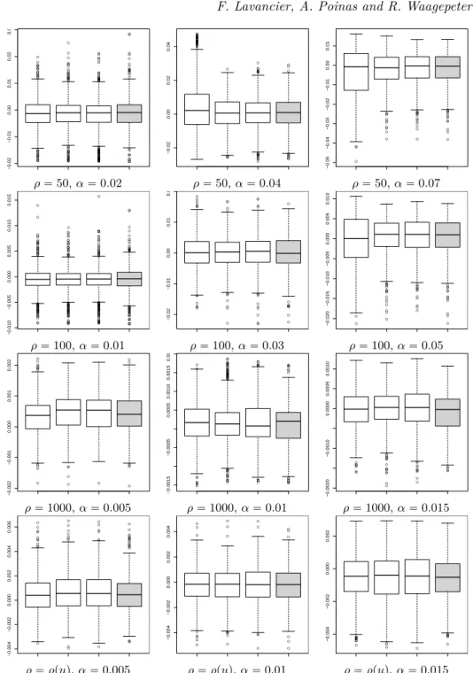
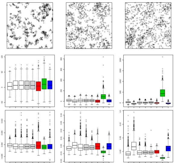
For this model, we consider three constant values of ρ, ρ P t50, 100, 1000u, correspond-ing to homogeneous DPPs, and an inhomogeneous situation where ρpuq “ ρpx, yq “ 20 expp4xq when u P r0, 1s2. The latter case corresponds to a log-linear intensity function involving two parameters. For each ρ, three values of α are considered: a small one, a medium one, and a last one close to the maximal possible value satisfying (7). Exam-ples of point patterns simulated on r0, 1s2 are displayed in Figure1. All simulations are carried out using R [21], in particular the library spatstat [1].
We estimate ρ and α by a two-step procedure as studied in Section3.2from realisations of the DPP on W “ r0, 1s2. The alternative global approach of Section3.1is discussed in
the next section. In the first step, the parameters arising in ρ are estimated by the score function for a Poisson point process. This gives ˆρ “ N pX X W q{|W | in the homogeneous
cases. In the second step, we consider the estimating equation based on (3) where θ is
α in this setting and when R P t0.05, 0.1, 0.25u, and based on the adaptive test function
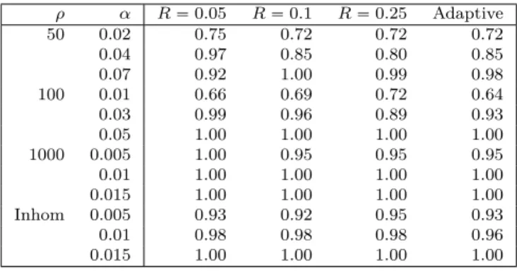
(4) with ε “ 0.01 and the weight function w given at the end of Section2.4. This yields four different estimators of α. The root mean square errors (RMSEs) of these estimators and the mean computation time estimated from 1000 replications are summarised in Table1. Boxplots are displayed in Figure S1in the supplementary material. Note that the codes have not been optimised, but the same computational strategy has been used for all methods, making the comparison of the mean computation time meaningful.
The Bessel-type kernel and the aforementioned test functions used in the two-step estimation procedure fulfill the assumptions of Theorem 3.4 and Lemma 3.5 (for the homogeneous case), ensuring nice asymptotic properties of the estimators considered
in this section. This is confirmed by the estimated RMSE’s reported in Table 1, that decrease when the intensity ρ increases [which mimics the effect of an increasing window since rescaling the window by a factor 1{k is equivalent to change ρ into k2ρ and α into
α{k, see (2.4) in8]. Moreover, these RMSE’s show that the best choice of R in the test
function (3) clearly depends on the range of interaction of the underlying process. This emphasizes the importance of a data-driven approach to choosing R since the range is unknown in practice. Fortunately, the performance of the adaptive method is, except for the case ρ “ 100, α “ 0.01, always better than the worst choice of R and very close to the best R. For the exceptional case, the small differences in performance can be explained by Monte Carlo error. Further, use of the adaptive method implies only little or no extra computional effort. In presence of many points, the adaptive version is in fact much faster to compute than the estimator based on (3) with the choice of a too large R, see for instance the results for ρ “ 1000 and R “ 0.25.
Table S2 in the supplementary material shows the root mean square errors of the adaptive estimator using ε “ 0.05. The RMSEs obtained with ε “ 0.05 are bigger than those obtained with ε “ 0.01. Nevertheless, the adaptive method with ε “ 0.05 still performs well in the sense that it usually performs better than the worst R and usually almost as good as the best R. Because the above estimation methods sometimes fail to converge, we also report in Table S1in the supplementary material the percentages of times each method has converged in our simulation study. These percentages are similar for all methods. Note that the results in Table 1 and in Figure S1 are based on 1000 simulations where all four methods have converged.
4.2. Two-step versus simultaneous
Most models used in spatial statistics involve a separable parameter θ “ pβ, ψq where β only appears in the intensity function and ψ only appears in the pair correlation func-tion. This makes the two-step procedure described in Section3.2available, as exploited in the previous simulation study. However a simultaneous second order estimating equation approach might be a better alternative. It is not easy to compare the respective perfor-mance of the two approaches through the asymptotic variances obtained in Section 3.1
and Section3.2. In this section, we show through an example why the two-step procedure seems preferable.
We consider a stationary model with parameter θ “ pρ, ψq, where ρ is the intensity and the pair correlation function writes gpu, v; θq “ gpr; ψq with r “ }u ´ v}. In this case the two-step procedure, based on the observation X X W and using the adaptive test function (4), provides ˆρ “ N pX X W q{|W | and ˆψ is the root of
e2pψq “ ÿ rij w ˆ ε gp0; ψq ´ 1 gprij; ψq ´ 1 ˙ ∇ψgprij; ψq gprij; ψq ´ N pX X W q2 ż W w ˆ εgp0; ψq ´ 1 gpr; ψq ´ 1 ˙ ∇ψgpr; ψqdF prq. (8)
● ● ● ● ● ● ● ● ● ● ● ● ● ● ● ● ● ● ● ● ● ● ● ● ● ● ● ● ● ● ● ● ● ● ● ● ● ● ● ● ● ● ● ● ● ● ● ● ● ● ● ● ● ● ● ● ● ● ● ● ● ● ● ● ● ● ● ● ● ● ● ● ● ● ● ● ● ● ● ● ● ● ● ● ● ● ● ● ● ● ● ● ● ● ● ● ● ● ● ● ● ● ● ● ● ● ● ● ● ● ● ● ● ● ● ● ● ● ● ● ● ● ● ● ● ● ● ● ● ● ● ● ● ● ● ● ● ● ● ● ● ● ● ● ● ● ● ● ● ρ “ 50, α “ 0.02 ρ “ 50, α “ 0.04 ρ “ 50, α “ 0.07 ● ● ● ● ● ● ● ● ● ● ● ● ● ● ● ● ● ● ● ● ● ● ● ● ● ● ● ● ● ● ● ● ● ● ● ● ● ● ● ● ● ● ● ● ● ● ● ● ● ● ● ● ● ● ● ● ● ● ● ● ● ● ● ● ● ● ● ● ● ● ● ● ● ● ● ● ● ● ● ● ● ● ● ● ● ● ● ● ● ● ● ● ● ● ● ● ● ● ● ● ● ● ● ● ● ● ● ● ● ● ● ● ● ● ● ● ● ● ● ● ● ● ● ● ● ● ● ● ● ● ● ● ● ● ● ● ● ● ● ● ● ● ● ● ● ● ● ● ● ● ● ● ● ● ● ● ● ● ● ● ● ● ● ● ● ● ● ● ● ● ● ● ● ● ● ● ● ● ● ● ● ● ● ● ● ● ● ● ● ● ● ● ● ● ● ● ● ● ● ● ● ● ● ● ● ● ● ● ● ● ● ● ● ● ● ● ● ● ● ● ● ● ● ● ● ● ● ● ● ● ● ● ● ● ● ● ● ● ● ● ● ● ● ● ● ● ● ● ● ● ● ● ● ● ● ● ● ● ● ● ● ● ● ● ● ● ● ● ● ● ● ● ● ● ● ● ● ● ● ● ● ● ● ● ● ● ● ● ● ● ● ● ● ● ● ● ● ● ● ● ● ● ● ● ● ● ● ● ● ● ● ● ● ● ● ● ● ● ● ρ “ 100, α “ 0.01 ρ “ 100, α “ 0.03 ρ “ 100, α “ 0.05 ● ● ● ● ● ● ● ● ● ● ● ● ● ● ● ● ● ● ● ● ● ● ● ● ● ● ● ● ● ● ●● ● ● ● ● ● ● ● ● ● ● ● ● ● ● ● ● ● ● ● ● ● ● ● ● ● ● ● ● ● ● ● ● ● ● ● ● ● ● ● ● ● ● ● ● ● ● ● ● ● ● ● ● ● ● ● ● ● ● ● ● ● ● ● ● ● ● ● ● ● ● ● ● ● ● ● ● ● ● ● ● ● ● ● ● ● ● ● ● ● ● ● ● ● ● ● ● ● ● ● ● ● ● ● ● ● ● ● ● ● ● ● ● ● ● ● ● ● ● ● ● ● ● ● ● ● ● ● ● ● ● ● ● ● ● ● ● ● ● ● ● ● ● ● ● ● ● ● ● ● ● ● ● ● ● ● ● ● ● ● ● ● ● ● ● ● ● ● ● ● ● ● ● ● ● ● ● ● ● ● ● ● ● ● ● ● ● ● ● ● ● ● ● ● ● ● ● ● ● ● ● ● ● ● ● ● ● ● ● ● ● ● ● ● ● ● ● ● ● ● ● ● ● ● ● ● ● ● ● ● ● ● ● ● ● ● ● ● ● ● ● ● ● ● ● ● ● ● ● ● ● ● ● ● ● ● ● ● ● ● ● ● ● ● ● ● ● ● ● ● ● ● ● ● ● ● ● ● ● ● ● ● ● ● ● ● ● ● ● ● ● ● ● ● ● ● ● ● ● ● ● ● ● ● ● ● ● ● ● ● ● ● ● ● ● ● ● ● ● ● ● ● ● ● ● ● ● ● ● ● ● ● ● ● ● ● ● ● ● ● ● ● ● ● ● ● ● ● ● ● ● ● ● ● ● ● ● ● ● ● ● ● ● ● ● ● ● ● ● ● ● ● ● ● ● ● ● ● ● ● ● ● ● ● ● ● ● ● ● ● ● ● ● ● ● ● ● ● ● ● ● ● ● ● ● ● ● ● ● ● ● ● ● ● ● ● ● ● ● ● ● ● ● ● ● ● ● ● ● ● ● ● ● ● ● ● ● ● ● ● ● ● ● ● ● ● ● ● ● ● ● ● ● ● ● ● ● ● ● ● ● ● ● ● ● ● ● ● ● ● ● ● ● ● ● ● ● ● ● ● ● ● ● ● ● ● ● ● ● ● ● ● ● ● ● ● ● ● ● ● ● ● ● ● ● ● ● ● ● ● ● ● ● ● ● ● ● ● ● ● ● ● ● ● ● ● ● ● ● ● ● ● ● ● ● ● ● ● ● ● ● ● ● ● ● ● ● ● ● ● ● ● ● ● ● ● ● ● ● ● ● ● ● ● ● ● ● ● ● ● ● ● ● ● ● ● ● ● ● ● ● ● ● ● ● ● ● ● ● ● ● ● ● ● ● ● ● ● ● ● ● ● ● ● ● ● ● ● ● ● ● ● ● ● ● ● ● ● ● ● ● ● ● ● ● ● ● ● ● ● ● ● ● ● ● ● ● ● ● ● ● ● ● ● ● ● ● ●● ● ● ● ● ● ● ● ● ● ● ● ● ● ● ● ● ● ● ● ● ● ● ● ● ● ● ● ● ● ● ● ● ● ● ● ● ● ● ● ● ● ● ● ● ● ● ● ● ● ● ● ● ● ● ● ● ● ● ● ● ● ● ● ● ● ● ● ● ● ● ● ● ● ● ● ● ● ● ● ● ● ● ● ● ● ● ● ● ● ● ● ● ● ● ● ● ● ● ● ● ● ● ● ● ● ● ● ● ● ● ● ● ● ● ● ● ● ● ● ● ● ● ● ● ● ● ● ● ●● ● ● ● ● ● ● ● ● ● ● ● ● ● ● ● ● ● ● ● ● ● ● ● ● ● ● ● ● ● ● ● ● ● ● ● ● ● ● ● ● ● ● ● ● ● ● ● ● ● ● ● ● ● ● ● ● ● ● ● ● ● ● ● ● ● ● ● ● ● ● ● ● ● ● ● ● ● ● ● ● ● ● ● ● ● ● ● ● ● ● ● ● ● ● ● ● ● ● ● ● ● ● ● ● ● ● ● ● ● ● ● ● ● ● ● ● ● ● ● ● ● ● ● ● ● ● ● ● ● ● ● ● ● ● ● ● ● ● ● ● ● ● ● ● ● ● ● ● ● ● ● ● ● ● ● ● ● ● ● ● ● ● ● ● ● ● ● ● ● ● ● ● ● ● ● ● ● ● ● ● ● ● ● ● ● ● ● ● ● ● ● ● ● ● ● ● ● ● ● ● ● ● ● ● ● ● ● ● ● ● ● ● ● ● ● ● ● ● ● ● ● ● ● ● ● ● ● ● ● ● ● ● ● ● ● ● ● ● ● ● ● ● ● ● ● ● ● ● ● ● ● ● ● ● ● ● ● ● ● ● ● ● ● ● ● ● ● ● ● ● ● ● ● ● ● ● ● ● ● ● ● ● ● ● ● ● ● ● ● ● ● ● ● ● ● ● ● ● ● ● ● ● ● ● ● ● ● ● ● ● ● ● ● ● ● ● ● ● ● ● ● ● ● ● ● ● ● ● ● ● ● ● ● ● ● ● ● ● ● ● ● ● ● ● ● ● ● ● ● ● ● ● ● ● ● ● ● ● ● ● ● ● ● ● ● ● ● ● ● ● ● ● ● ● ● ● ●● ● ● ● ● ● ● ● ● ● ● ● ● ● ● ● ● ● ● ● ● ● ● ● ● ● ● ● ● ● ● ● ● ● ● ● ● ● ● ● ● ● ● ● ● ● ● ● ● ● ● ● ● ● ● ● ● ● ● ● ● ● ● ● ● ● ● ● ● ● ● ● ● ● ● ● ● ● ● ● ● ● ● ● ● ● ● ● ● ● ● ● ● ● ● ● ● ● ● ● ● ● ● ● ● ● ● ● ● ● ● ● ● ● ● ● ● ● ● ● ● ● ● ● ● ● ● ● ● ● ● ● ● ● ● ● ● ● ● ● ● ● ● ● ● ● ● ● ● ● ● ● ● ● ● ● ● ● ● ● ● ● ● ● ● ● ● ● ● ● ● ● ● ● ● ● ● ● ● ● ● ● ● ● ● ● ● ● ● ● ● ● ● ● ● ● ● ● ● ● ● ● ● ● ● ● ● ● ● ● ● ● ● ● ● ● ● ● ● ● ● ● ● ● ● ● ● ● ● ● ● ● ● ● ● ● ● ● ● ● ● ● ● ● ● ● ● ● ● ● ● ● ● ● ● ● ● ● ● ● ● ● ● ● ● ● ● ● ● ● ● ● ● ● ● ● ● ● ● ● ● ● ● ● ● ● ● ● ● ● ● ● ● ● ● ● ● ● ● ● ● ● ● ● ● ● ● ● ● ● ● ● ● ● ● ● ● ● ● ● ● ● ● ● ● ● ● ● ● ● ● ● ● ● ● ● ● ● ● ● ● ● ● ● ● ● ● ● ● ● ● ● ● ● ● ● ● ● ● ● ● ● ● ● ● ● ● ● ● ● ● ● ● ● ● ● ● ● ● ● ● ● ● ● ● ● ● ● ● ● ● ● ● ● ● ● ● ● ● ● ● ● ● ● ● ● ● ● ● ● ● ● ● ● ● ● ● ● ● ● ● ● ● ● ● ● ● ● ● ● ● ● ● ● ● ● ● ● ● ● ● ● ● ● ● ● ● ● ● ● ● ● ● ● ● ● ● ● ● ● ● ● ● ● ● ● ● ● ● ● ● ● ● ● ● ● ● ● ● ● ● ● ● ● ● ● ● ● ● ● ● ● ● ● ● ● ● ● ● ● ● ● ● ● ● ● ● ● ● ● ● ● ● ● ● ● ● ● ● ● ● ● ● ● ● ● ● ● ● ● ● ● ● ● ● ● ● ● ● ● ● ● ● ● ● ● ● ● ● ● ● ● ● ● ● ● ● ● ● ● ● ● ● ● ● ● ● ● ● ● ● ● ● ● ● ● ● ● ● ● ● ● ● ● ● ● ● ● ● ● ● ● ● ● ● ● ● ● ● ● ● ● ● ● ● ● ● ● ● ● ● ● ● ● ● ● ● ● ● ● ● ● ● ● ● ● ● ● ● ● ● ● ● ● ● ● ● ● ● ● ● ● ● ● ● ● ● ● ● ● ● ● ● ● ● ● ● ● ● ● ● ● ● ● ● ● ● ● ● ● ● ● ● ● ● ● ● ● ● ● ● ● ● ● ● ● ● ● ● ● ● ● ● ● ● ● ● ● ● ● ● ● ● ● ● ● ● ● ● ● ● ● ● ● ● ● ● ● ● ● ● ● ● ● ● ● ● ● ● ● ● ● ● ● ● ● ● ● ● ● ● ● ● ● ● ● ● ● ● ● ● ● ● ● ● ● ● ● ● ● ● ● ● ● ● ● ● ● ● ● ● ● ● ● ● ● ● ● ● ● ● ● ● ● ● ● ● ● ● ● ● ● ● ● ● ● ● ● ● ● ● ● ● ● ● ● ● ● ● ● ● ● ● ● ● ● ● ● ● ● ● ● ● ● ● ● ● ● ● ● ● ● ● ● ● ● ● ● ● ● ● ● ● ● ● ● ● ● ● ● ● ● ● ● ● ● ● ● ● ● ● ● ● ● ● ● ● ● ● ● ● ● ● ● ● ● ● ● ● ● ● ● ● ● ● ● ● ● ● ● ● ● ● ● ● ● ● ● ● ● ● ● ● ● ● ● ● ● ● ● ● ● ● ● ● ● ● ● ● ● ● ● ● ● ● ● ● ● ● ● ● ● ● ● ● ● ● ● ● ● ● ● ● ● ● ● ● ● ● ● ● ● ● ● ● ● ● ● ● ● ● ● ● ● ● ● ● ● ● ● ● ● ● ● ● ● ● ● ● ● ● ● ● ● ● ● ● ● ● ● ● ● ● ● ● ● ● ● ● ● ● ● ● ● ● ● ● ● ● ● ● ● ● ● ● ● ● ● ● ● ● ● ● ● ● ● ● ● ● ● ● ● ● ● ● ● ● ● ● ● ● ● ● ● ● ● ● ● ● ● ● ● ● ● ● ● ● ● ● ● ● ● ● ● ● ● ● ● ● ● ● ● ● ● ● ● ● ● ● ● ● ● ● ● ● ● ● ● ● ● ● ● ● ● ● ● ● ● ● ● ● ● ● ● ● ● ● ● ● ● ● ● ● ● ● ● ● ● ● ● ● ● ● ● ● ● ● ● ● ● ● ● ● ● ● ● ● ● ● ● ● ● ● ● ● ● ● ● ● ● ● ● ● ● ● ● ●● ● ● ● ● ● ● ● ● ● ● ● ● ● ● ● ● ● ● ● ● ● ● ● ● ● ● ● ● ● ● ● ● ● ● ● ● ● ● ● ● ● ● ● ● ● ● ● ● ● ● ● ● ● ● ● ● ● ● ● ● ● ● ● ● ● ● ● ● ● ● ● ● ● ● ● ● ● ● ● ● ● ● ● ● ● ● ● ● ● ● ● ● ● ● ● ● ● ● ● ● ● ● ● ● ● ● ● ● ● ● ● ● ● ● ● ● ● ● ● ● ● ● ● ● ● ● ● ● ● ● ● ● ● ● ● ● ● ● ● ● ● ● ● ● ● ● ● ● ● ● ● ● ● ● ● ● ● ● ● ● ● ● ● ● ● ● ● ● ● ● ● ● ● ● ● ● ● ● ● ● ● ● ● ● ● ● ● ● ● ● ● ● ● ● ● ● ● ● ● ● ● ● ● ● ● ● ● ● ● ● ● ● ● ● ● ● ● ● ● ● ● ● ● ● ● ● ● ● ● ● ●● ● ● ● ● ● ● ● ● ● ● ● ● ● ● ● ● ● ● ● ● ● ● ● ● ● ● ● ● ● ● ● ● ● ● ● ● ● ● ● ● ● ● ● ● ● ● ● ● ● ● ● ● ● ● ● ● ● ● ● ● ● ● ● ● ● ● ● ● ● ● ● ● ● ● ● ● ● ● ● ● ● ● ● ● ● ● ● ● ● ● ● ● ● ● ● ● ● ● ● ● ● ● ● ● ● ● ● ● ● ● ● ● ● ● ● ● ● ● ● ● ● ● ● ● ● ● ● ● ● ● ● ● ● ● ● ● ● ● ● ● ● ● ● ● ● ● ● ● ● ● ● ● ● ● ● ● ● ● ● ● ● ● ● ● ● ● ● ● ● ● ● ● ● ● ● ● ● ● ● ● ● ● ● ● ● ● ● ● ● ● ● ● ● ● ● ●● ● ● ● ● ● ● ● ● ● ● ● ● ● ● ● ● ● ● ● ● ● ● ● ● ● ● ● ● ● ● ● ● ● ● ● ● ● ● ● ● ● ● ● ● ● ● ● ● ● ● ● ● ● ● ● ● ● ● ● ● ● ● ● ● ● ● ● ● ● ● ● ● ● ● ● ● ● ● ● ● ● ● ● ● ● ● ● ● ● ● ● ● ● ● ● ● ● ● ● ● ● ● ● ● ● ● ● ● ● ● ● ● ● ● ● ● ● ● ● ● ● ● ● ● ● ● ● ● ● ● ● ● ● ● ● ● ● ● ● ● ● ● ● ● ● ● ● ● ● ● ● ● ● ● ● ● ● ● ● ● ● ● ● ● ● ● ● ● ● ● ● ● ● ● ● ● ● ● ● ● ● ● ● ● ● ● ● ● ● ● ● ● ● ● ● ● ● ● ● ● ● ● ● ● ● ● ● ● ● ● ● ● ● ● ● ● ● ● ● ● ● ● ● ● ● ● ● ● ● ● ● ● ● ● ● ● ● ● ● ● ● ● ● ● ● ● ● ● ● ● ● ● ● ● ● ● ● ● ● ● ● ● ● ● ● ● ● ● ● ● ● ● ● ● ● ● ● ● ρ “ 1000, α “ 0.005 ρ “ 1000, α “ 0.01 ρ “ 1000, α “ 0.015 ● ● ● ● ● ● ● ● ● ● ● ● ● ● ● ● ● ● ● ● ● ● ● ● ● ● ● ● ● ● ● ● ● ● ● ● ● ● ● ● ● ● ● ● ● ● ● ● ● ● ● ● ● ● ● ● ● ● ● ● ● ● ● ● ● ● ● ● ● ● ● ● ● ● ● ● ● ● ● ● ● ● ● ● ● ● ● ● ● ● ● ● ● ● ● ● ● ● ● ● ● ● ● ● ● ● ● ● ● ● ● ● ● ● ● ● ● ● ● ● ● ● ● ● ● ● ● ● ● ● ● ● ● ● ● ● ● ● ● ● ● ● ● ● ● ● ● ● ● ● ● ● ● ● ● ● ● ● ● ● ● ● ● ● ● ● ● ● ● ● ● ● ● ● ● ● ● ● ● ● ● ● ● ● ● ● ● ● ● ● ● ● ● ● ● ● ● ● ● ● ● ● ● ● ● ● ● ● ● ● ● ● ● ● ● ● ● ● ● ● ● ● ● ● ● ● ● ● ● ● ● ● ● ● ● ● ● ● ● ● ● ● ● ● ● ● ● ● ● ● ● ● ● ● ● ● ● ● ● ● ● ● ● ● ● ● ● ● ● ● ● ● ● ● ● ● ● ● ● ● ● ● ● ● ● ● ● ● ● ● ● ● ● ● ● ● ● ● ● ● ● ● ● ● ● ● ● ● ● ● ● ● ● ● ● ● ● ● ●● ● ● ● ● ● ● ● ● ● ● ● ● ● ● ● ● ● ● ● ● ● ● ● ● ● ● ● ● ● ● ● ● ● ● ● ● ● ● ● ● ● ● ● ● ● ● ● ● ● ● ● ● ● ● ● ● ● ● ● ● ● ● ● ● ● ● ● ● ● ● ● ● ● ● ● ● ● ● ● ● ● ● ● ● ● ● ● ● ● ● ● ● ● ● ● ● ● ● ● ● ● ● ● ● ● ● ● ● ● ● ● ● ● ● ● ● ● ● ● ● ● ● ● ● ● ● ● ● ● ● ● ● ● ● ● ● ● ● ● ● ● ● ● ● ● ● ● ● ● ● ● ● ● ● ● ● ● ● ● ● ● ● ● ● ● ● ● ● ● ● ● ● ● ● ● ● ● ● ● ● ● ● ● ● ● ● ● ● ● ● ● ● ● ● ● ● ● ● ● ● ● ● ● ● ● ● ● ● ● ● ● ● ● ● ● ● ● ● ● ● ● ● ● ● ● ● ● ● ● ● ● ● ● ● ● ● ● ● ● ● ● ● ● ● ● ● ● ● ● ● ● ● ● ● ● ● ● ● ● ● ● ● ● ● ● ● ● ● ● ● ● ● ● ● ● ● ● ● ● ● ● ● ● ● ● ● ● ● ● ● ● ● ● ● ● ● ● ● ● ● ● ● ● ● ● ● ● ● ● ● ● ● ● ● ● ● ● ● ● ● ● ● ● ● ● ● ● ● ● ● ● ● ● ● ● ● ● ● ● ● ● ● ● ● ● ● ● ● ● ● ● ● ● ● ● ● ● ● ● ● ● ● ● ● ● ● ● ● ● ● ● ● ● ● ● ● ● ● ● ● ● ● ● ● ● ● ● ● ● ● ● ● ● ● ● ● ● ● ● ● ● ● ● ● ● ● ● ● ● ● ● ● ● ● ● ● ● ● ● ● ● ● ● ● ● ● ● ● ● ● ● ● ● ● ● ● ● ● ● ● ● ● ● ● ● ● ● ● ● ● ● ● ● ● ● ● ● ● ● ● ● ● ● ● ● ● ● ● ● ● ● ● ● ● ● ● ● ● ● ● ● ● ● ● ● ● ● ● ● ● ● ● ● ● ● ● ● ● ● ● ● ● ● ● ● ● ● ● ● ● ● ●
ρ “ ρpuq, α “ 0.005 ρ “ ρpuq, α “ 0.01 ρ “ ρpuq, α “ 0.015
Figure 1.Examples of point patterns simulated from a Bessel-type DPP on r0, 1s2 for different values of ρ and α. For the last row, ρpx, yq “ 20 expp4xq.
ρ α R “ 0.05 R “ 0.1 R “ 0.25 Adaptive Rˆ 50 0.02 rmse: 5.84 5.83 6.29 5.97 0.047 (0.15) (0.17) (0.19) (0.18) (0.020) time: 0.43 0.48 0.68 0.64 0.04 rmse: 15.60 9.18 9.19 9.25 0.106 (0.44) (0.20) (0.22) (0.21) (0.037) time: 0.48 0.50 0.68 0.73 0.07 rmse: 13.32 8.25 8.22 8.15 0.147 (0.33) (0.23) (0.24) (0.24) (0.050) time: 0.50 0.45 0.59 0.72 100 0.01 rmse: 2.44 2.45 2.58 2.63 0.024 (0.08) (0.08) (0.09) (0.09) (0.009) time: 0.44 0.57 1.22 0.70 0.03 rmse: 5.34 5.12 5.28 5.27 0.064 (0.13) (0.13) (0.14) (0.13) (0.019) time: 0.40 0.47 0.98 0.70 0.05 rmse: 5.78 4.43 4.50 4.53 0.139 (0.12) (0.12) (0.10) (0.12) (0.022) time: 0.52 0.56 1.16 0.95 1000 0.005 rmse: 0.67 0.88 0.83 0.72 0.015 (0.02) (0.02) (0.02) (0.02) (0.003) time: 3.83 19.04 110.07 9.38 0.01 rmse: 0.57 0.59 0.61 0.56 0.028 (0.01) (0.02) (0.01) (0.01) (0.005) time: 2.68 10.40 60.79 6.84 0.015 rmse: 0.47 0.46 0.52 0.47 0.026 (0.01) (0.01) (0.01) (0.01) (0.002) time: 2.53 9.81 55.78 7.75 Inhom 0.005 rmse: 1.58 1.65 1.66 1.61 0.014 (0.04) (0.04) (0.04) (0.04) (0.005) time: 0.89 2.50 10.30 1.19 0.01 rmse: 1.34 1.36 1.36 1.32 0.025 (0.03) (0.03) (0.03) (0.03) (0.008) time: 0.76 1.86 7.66 1.22 0.015 rmse: 1.43 1.47 1.48 1.40 0.030 (0.03) (0.03) (0.03) (0.03) (0.006) time: 0.86 1.90 7.46 1.40
Table 1. Estimated root mean square errors (ˆ103) and mean computation time (in seconds) of ˆα for a Bessel-type DPP on r0, 1s2, for different values of ρ and α. The 3 first estimators use
the test function (3) with R “ 0.05, R “ 0.1 and R “ 0.25 respectively, while the last estimator is the adaptive version based on (4). The standard errors of the RMSE estimations are given in parenthesis. The last column gives the averages of ”practical ranges” (i.e. maximal
solution to |gprq ´ 1| “ 0.01) used for the adaptive estimator, along with their standard deviations in parenthesis. For each value of ρ and α, these quantities are computed from 1000
Here F denotes the cumulative distribution function of R “ }U ´ V } where U and V are independent variables uniformly distributed on W and triju is the set of all pairwise
distances of X X W . On the other hand, by a simultaneous procedure using the same test function, we get that ˆψ is the root of
epψq “ÿ rij w ˆ ε gp0; ψq ´ 1 gprij; ψq ´ 1 ˙ ∇ψgprij; ψq gprij; ψq ´ ř rijw ´ ε gp0;ψq´1 gprij;ψq´1 ¯ ş w´ε gp0;ψq´1 gprij;ψq´1 ¯ gpr; ψqdF prq ż w ˆ ε gp0; ψq ´ 1 gprij; ψq ´ 1 ˙ ∇ψgpr; ψqdF prq, (9) while ˆρ is given by ˆ ρ2“ 1 |W |2 ř rijw ´ ε gp0; ˆψq´1 gprij; ˆψq´1 ¯ ş w´ε gp0; ˆψq´1 gprij; ˆψq´1 ¯ gpr; ˆψqdF prq . (10)
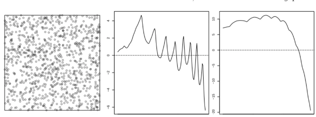
The more complicated expression of (9) in comparison with (8) implies that epψq can be highly irregular in ψ. FigureS2in the supplementary material shows an example for one realisation of a DPP with a Gaussian kernel with range ψ. For this example epψq exhibits many different roots, although the dataset contains a fairly large number of points (about 1000). The consequence is an extreme sensitivity to the initial parameter when we try to solve epψq “ 0. In contrast e2pψq “ 0 has one clear solution. This
advocates the use of the two-step approach.
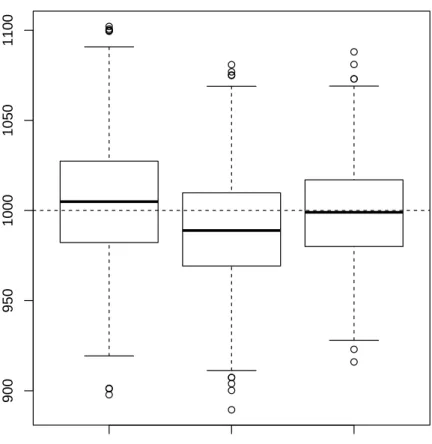
Due to the aforementioned very strong sensitivity to the initial value of ψ, conclusions from comparison of the simultaneous estimate of ψ with the two-step estimate of ψ can be quite arbitrary. However, we report in FigureS3in the supplementary material the distribution of estimates of ρ from 1000 simulations of a Bessel-type DPP with
ρ “ 1000 and ψ “ α “ 0.01, using either (10) from the simultaneous approach or ˆρ “
N pX XW q{|W | from the two-step approach. For the simultaneous method we either chose
the true value α “ 0.01 as the starting point for the numerical solution of epαq “ 0 to get ˆ
α, or fixed ˆα at the true value, i.e. ˆα “ 0.01, in (10). The estimate ˆρ “ N pX X W q{|W |
is unequivocally better than (10) in terms of root mean square error, even when the true value of α is used for ˆα in (10). This confirms our recommendation.
The simultaneous estimation approach in this example is covered by our theoretical results in Sections3.1and3.2. It shows that while our consistency result guarantees the existence of a consistent sequence of parameter estimates (roots) there could also exist other non-consistent sequences.
5. Discussion
In this paper we provide a very general asymptotic framework for estimating function inference for spatial point processses with known joint intensities. Specific asymptotic results are obtained for determinantal point processes.
The performance of second order estimating functions depends strongly on a tuning parameter that controls which pairs of points are used in the estimation. Our adaptive choice of this tuning parameter is intuitively appealing, easy to implement and performs well in the simulation studies considered. It moreover seamlessly integrates with the asymptotic results where the use of the adaptive method poses no extra theoretical difficulties. Though we focus in this paper on determinantal point processes, the adaptive method is applicable for any spatial point process with known pair correlation function. As an example we provide in Section3of the supplementary material a simulation study in case of a cluster process.
Appendix A: Assumptions and proof of Theorem
2.1
Our general Theorem2.1depends on a number of assumptions. The setting is the same as in Section2.2. We moreover define diampxq as the largest distance between two coor-dinates of x. The assumptions (F1) through (F3) are mainly related to the test functions
fi, while for X we assume (X1) through (X3).
(F1) For all i “ 1, . . . , l and for all x P pRdqqi, θ ÞÑ f
ipx; θq is twice continuously
differentiable in a neighbourhood of θ˚. Moreover, the first and second derivative
of fi with respect to θ are bounded with respect to x P pRdqqi uniformly in θ
belonging to this neighbourhood.
(F2) There exists a constant R ą 0 such that for all θ in a neighbourhood of θ˚, all
functions x ÞÑ fipx; θq vanish when diampxq ą R.
Define the matrices Hnpθq by
Hnpθq “ ¨ ˚ ˝ H1 npθq .. . Hl npθq ˛ ‹ ‚,
where for all i
Hnipθq :“ 1 |Wn|
ż
Wnqi
fipx; θq∇θρpqiqpx; θqTdx.
(F3) The matrices Hnpθ˚q satisfy
lim inf nÑ8 ˆ inf }φ}“1 φTHnpθ˚qφ ˙ ą 0.
(F3’) There exists a neighbourhood of θ˚ such that for all n high enough and all θ in
this neighbourhood, Hnpθq is invertible and }Hnpθq´1} is uniformly bounded with
respect to n and θ, where } ¨ } stands for any matrix norm. (X1) For all θ in a neighbourhood of θ˚ and all q
i, i “ 1, . . . , l, the intensity functions
continuously differentiable in a neighbourhood of θ˚, for all x P pRd
qqi. Finally, the
first and second derivative of ρpqiq with respect to θ are bounded with respect to
x P pRd
qqi uniformly in θ belonging to this neighbourhood.
(X2) For all qi, i “ 1, . . . , l, the intensity functions ρpqiqp¨; θ˚q, ¨ ¨ ¨ , ρp2qiqp¨; θ˚q of X are
well-defined. Moreover, the intensity functions ρpqiqp¨; θ˚q, ¨ ¨ ¨ , ρp2qi´1qp¨; θ˚q are
bounded and for all bounded sets W Ă Rd there exists a constant C
0ą 0, so that
ş
Wϕipx1qdx1ă C0, i “ 1, . . . , l where ϕi is the function
ϕi: x1ÞÑ sup diampxqăR sup diampyqăR sup y1PW ρp2qiqpx 1, x2, ¨ ¨ ¨ , xqi, y1, ¨ ¨ ¨ , yqi; θ ˚ q ´ ρpqiqpx1, x2, ¨ ¨ ¨ , x qi; θ ˚qρpqiqpy1, ¨ ¨ ¨ , y qi; θ ˚q
with R coming from (F2).
(X3) X satisfies the central limit theorem Σ´1{2n enpθ˚q
L
ÝÑ N p0, Ipq,
where en is defined in Section 2.2and Σn“ Varpenpθ˚qq.
Assumptions (F1) and (F2) are basic regularity conditions on the fi’s. Similarly (X1)
and (X2) ensure that the intensity functions of X exist and are sufficiently regular. The technical assumptions are in fact (F3) (or (F3’)) and (X3). While the latter strongly de-pends on the underlying point process (see [23] for Cox processes and [14] for DPPs), the former can be simplified in some cases. For example, if Hnpθ˚q are symmetrical matrices
for all n then (F3) writes lim infnλminpHnpθ˚qq ą 0 where λminpHnpθ˚qq denotes the
smallest eigenvalue of Hnpθ˚q. If the matrices Hnpθ˚q are not symmetrical, Assumption
(F3’) will be preferred since (F3) does not translate well for non-symmetrical matrices. Furthermore, if X is stationary and all fi’s are invariant by translation, then Hnpθq
con-verges towards a matrix Hpθq explicitly given in Lemma A.1 below, thus Assumption (F3) simply becomes inf}φ}“1φTHpθ˚qφ ą 0 and (F3’) is satisfied whenever Hpθ˚q is
invertible by continuity of Hpθq.
Lemma A.1. Assume (W), (X1), (F2) and let θ P Rp. Suppose that all ρpqiqp¨; θq’s and
fip¨; θq’s are invariant by translation, i.e. fipu1, u; θq “ fip0, u ´ u1; θq where we denote
by u the vector pu2, ¨ ¨ ¨ , uqiq. If u ÞÑ fip0, u; θq is integrable for all i such that qi ě 2,
then Hnpθq converges to a matrix Hpθq. In particular, for all i we have
lim nÑ8H i npθq “ ż }t}ďR fip0, t; θq∇θρpqiqp0, t; θqTdt.
This lemma is verified in Section B. We now turn to the proof of the theorem. To prove the consistency of ˆθn and get its rate of convergence we apply the following result,
Theorem A.2 ([23]). Suppose that enpθq is continuously differentiable with respect to θ and define Jnpθq :“ ´ d dθTenpθq :“ ´ ˆ B Bθj enpθqi ˙ 1ďi,jďp . Suppose that for all α ą 0
sup θPMα npθ˚q › › › › 1 |Wn| pJnpθq ´ Jnpθ˚qq › › › › P ÝÑ 0, (11) where Mnαpθ˚q :“ # θ P Θ : }θ ´ θ˚} ď aα |Wn| + , and suppose that there exists l ą 0 such that
P ˆ 1 |Wn| inf }φ}“1 φTJnpθ˚qφ ă l ˙ Ñ 0. (12)
Assume, moreover, that the class of random vectors
# 1 a |Wn| enpθ˚q : n P N +
is stochastically bounded. Then, for all ε ą 0, there exists d ą 0 such that
PpDθˆn : enpˆθnq “ 0 and |Wn|}ˆθn´ θ˚} ă dq ą 1 ´ ε (13)
for a sufficiently large n.
We now verify the assumptions of Theorem A.2. There is no loss in generality by assuming that all fi are symmetric functions. Otherwise we can just replace fipxq by
its symmetrized version pqi!q´1řuPπpxqfipuq where πpxq denotes the set of all vectors
obtained by permuting the components of x. This does not change the value of enpθq and
each symmetrized function still satisfies Assumptions (F1) through (F3). We will use at several places the following result.
Lemma A.3. Let X be a point process satisfying Assumption (X2). Consider any i P t1, ¨ ¨ ¨ , lu, any bounded set W Ă Rd, and any symmetric bounded function g : pRd
qqi Ñ
Rki vanishing when two of its components are at a distance greater than R for a given
constant R ą 0. Then › › › › › › Var ¨ ˝ ‰ ÿ x1,¨¨¨ ,xqiPXXW gpx1, ¨ ¨ ¨ , xqiq ˛ ‚ › › › › › › “ Op|W |q.
Proof. Since g is a symmetric function, then gpx1, ¨ ¨ ¨ , xqiq does not depend on the order
of the xi. Thus, for any set of qipoints S “ tx1, ¨ ¨ ¨ , xqiu, we can write gpSq for the value
of g at an arbitrary order of the points in S and we write
‰ ÿ x1,¨¨¨ ,xqiPXXW gpx1, ¨ ¨ ¨ , xqiq “ qi! ÿ SĂXXW gpSq1|S|“qi. We start by expanding E“`řSĂXXWgpSq1|S|“qi ˘ `ř SĂXXWg T pSq1|S|“qi ˘‰ as qi ÿ k“0 E » — — – ÿ S,T ĂXXW |S|“|T |“qi,|SXT |“k gpSqgTpT q fi ffi ffi fl “ qi ÿ k“0 E » — — – ÿ U ĂXXW |U |“2qi´k ÿ S1ĂSĂU |S1|“k,|S|“qi gpSqgTpS1Y pU zSqq fi ffi ffi fl “ qi ÿ k“0 1 p2qi´ kq! ż W2qi´k ÿ S1ĂSĂtx1,¨¨¨ ,x2qi´ku |S1|“k,|S|“qi gpSqgTpS1Y ptx1, ¨ ¨ ¨ , x2qi´kuzSqqρ p2qi´kq px; θ˚qdx “ qi ÿ k“0 `qi k ˘`2qi´k qi ˘ p2qi´ kq! ż W2qi´k gpx1, ¨ ¨ ¨ , xqiqg T px1, ¨ ¨ ¨ , xk, xqi`1, ¨ ¨ ¨ , x2qi´kqρ p2qi´kqpx; θ˚qdx. (14) By Assumption (X2), the functions ρpqiq, ¨ ¨ ¨ , ρp2qi´1q are all bounded. Moreover, as a
consequence of our assumptions on g, each component of each term for k ě 1 in (14) is bounded by 1 qi!pqi´ kq! ˆqi k ˙ ż W2qi´k }g}28}ρp2qi´kq} 81t0ď|xi´x1|ďR, @iudx
which is Op|W |q. However, for k “ 0, the term is Op|W |2
q. Instead of controlling this term alone, we consider its difference with the remaining term in the variance we are looking at, that is
1 pqi!q2 ż W2qi gpxqgTpyqρp2qiqpx, y; θ˚qdxdy ´ E « ÿ SĂXXW gpSq1|S|“qi ff E « ÿ SĂXXW gpSq1|S|“qi ffT “ 1 pqi!q2 ż W2qi