Title
:
software
Auteurs:
Authors
:
Maxime Ouellet, François Gauthier, Ettore Merlo, Neset Sozen et
Martin Gagnon
Date: 2012
Type:
Rapport / ReportRéférence:
Citation
:
Ouellet, M., Gauthier, F., Merlo, E., Sozen, N. & Gagnon, M. (2012). Mapping features to source code in dynamically configured avionics software (Rapport technique n° EPM-RT-2012-02).
Document en libre accès dans PolyPublie
Open Access document in PolyPublie URL de PolyPublie:
PolyPublie URL: http://publications.polymtl.ca/2796/
Version: Version officielle de l'éditeur / Published versionNon révisé par les pairs / Unrefereed Conditions d’utilisation:
Terms of Use: Tous droits réservés / All rights reserved
Document publié chez l’éditeur officiel
Document issued by the official publisher Maison d’édition:
Publisher: École Polytechnique de Montréal
URL officiel:
Official URL: http://publications.polymtl.ca/2796/
Mention légale:
Legal notice:
Ce fichier a été téléchargé à partir de PolyPublie, le dépôt institutionnel de Polytechnique Montréal
This file has been downloaded from PolyPublie, the institutional repository of Polytechnique Montréal
MAPPING FEATURES TO SOURCE CODE IN
DYNAMICALLY CONFIGURED AVIONICS SOFTWARE
Maxime Ouellet, François Gauthier, Ettore Merlo, Neset Sozen,
Martin Gagnon
Département de Génie informatique et génie logiciel
École Polytechnique de Montréal
CMC Electronics Inc
EPM-RT-2012-02
MAPPING FEATURES TO SOURCE CODE IN
DYNAMICALLY CONFIGURED AVIONICS SOFTWARE
Maxime Ouellet
1, François Gauthier
1, Ettore Merlo
1,
Neset Sozen
1,2, Martin Gagnon
21
Département de génie informatique et génie logiciel
École Polytechnique de Montréal
2
CMC Electronics Inc.
2012
Maxime Ouellet, François Gauthier, Ettore Merlo, Neset Sozen, Martin Gauthier
Tous droits réservés
Dépôt légal :
Bibliothèque nationale du Québec, 2012 Bibliothèque nationale du Canada, 2012
EPM-RT-2012-02
Mapping features to source code in dynamically configured avionics software
par : Maxime Ouellet, François Gauthier, Ettore Merlo, Neset Sozen, Martin Gauthier Département de génie informatique et génie logiciel
École Polytechnique de Montréal
Toute reproduction de ce document à des fins d'étude personnelle ou de recherche est autorisée à la condition que la citation ci-dessus y soit mentionnée.
Tout autre usage doit faire l'objet d'une autorisation écrite des auteurs. Les demandes peuvent être adressées directement aux auteurs (consulter le bottin sur le site http://www.polymtl.ca/) ou par l'entremise de la Bibliothèque :
École Polytechnique de Montréal
Bibliothèque – Service de fourniture de documents Case postale 6079, Succursale «Centre-Ville» Montréal (Québec)
Canada H3C 3A7
Téléphone : (514) 340-4846 Télécopie : (514) 340-4026
Courrier électronique : biblio.sfd@courriel.polymtl.ca
Ce rapport technique peut-être repéré par auteur et par titre dans le catalogue de la Bibliothèque :
Mapping features to source code in dynamically configured
avionics software
Maxime Ouellet
1, Franc¸ois Gauthier
1, Ettore Merlo
1, Neset Sozen
1,2, Martin Gagnon
2 1Computer and Software Engineering Department, ´Ecole Polytechnique de Montr´eal, Canada2CMC Electronics Inc., Saint-Laurent, Quebec, Canada
SUMMARY
Mapping software features to the code that implements them is an important activity for program comprehension and software reengineering. In this paper, we present a novel automated approach to locate features in source code based on static analysis and model checking. This approach focuses on dynamically configured software in which the activation of specific features is controlled by configuration variables. The main advantages of a static approach to feature location are its affordability and applicability to large systems containing hundreds of features. Our methodology is applied to an industrial Flight Management System from the avionics industry. Results show that a static approach to feature mapping is feasible and can locate complex features whose implementation is spread across multiple files and functions.
1. INTRODUCTION
Model-driven engineering allows companies to model software and then generate their systems from models. For companies whose products share a common base, Software Product Line (SPL) models can improve reuse of software assets by benefiting from inter-product commonalities. In order to reuse software assets, companies may want to consider their existing legacy systems while building their new SPL models. This is especially true in the avionics industry, where complex algorithms implementing specific features must be reused in future generations of software. An approach that can help with this perspective is to map implemented features to the legacy code that implements them, thus allowing the reengineering team to quickly find which algorithms to reuse.
System properties and characteristics that are relevant to stakeholders and understandable by both customers and developers, are often referred to as features the product has or delivers. Features can be used to describe commonalities, differences, and variability between systems [1]. They are typically divided into functional and non-functional features. Functional features include services, which are marketable units or units of increment in a product line, and operations, which are internal product functions needed to provide services. Nonfunctional features include distinguishable system characteristics that are not naturally, easily, or intuitively identified in terms of services or operations, such as presentation, capacity, usage, cost, and other quality attributes such as safety, reliability, scalability, performance and portability [2].
In this paper, we refer to the implementation of a feature as the set of source code statements participating in the realization of such a feature. The relation between a feature and its implementation is called feature mapping, while locating features is the process of computing such a feature mapping.
Avionic systems usually have to support a wide range of aircraft, so they are sometimes implemented as dynamically configured software. With this type of system, the products for all supported aircrafts are located within the same implementation, and features are activated or deactivated through conditions in the code. Locating features in dynamically configured software
is important, since the implementation of a specific feature may be distributed across multiple files and multiple functions, making features hard to locate efficiently across large software. Knowing where specific features are implemented is also interesting in the context of software evolution. Software systems may evolve due to bug fixes, the need to improve the software or some environment changes, such as new standards. In all these cases, identifying sections of source code that implement a feature can be of great help to the developers, as concluded in [3].
Different approaches to locate features in source code have been proposed, as described in section 2.1. However, none can easily be applied to dynamically configured real-time software that exists in the avionics industry. Since real-time avionics software must be executed on specialized hardware with limited accessibility, approaches that include dynamic analysis are expensive to apply, both in time and money. Static feature location techniques are therefore of great interest for this industry because of their affordability. The code instrumentation necessary for dynamic analysis may also alter timing specifications of those systems. Moreover, even if dynamic analysis of the software were possible, the number of features and the complexity of decades old legacy software make dynamic analysis difficult to accomplish, since those techniques require the development of specialized test cases to be developed for each feature.
This article proposes an automated feature mapping technique for dynamically configured software based on static analysis and model checking. Our research objectives are to (1) define an automated feature mapping technique based on static analysis, and (2) evaluate this technique on an industrial software program.
This paper is organized as follows. Section 2 lists the research related to our work. Section 3 gives the necessary background for our approach. Section 4 introduces the goal of our methodology and the necessary conditions. Section 5 describes our methodology of our feature location technique. Section 6 presents the results from applying our methodology to an industrial system, the FMS. Section 7 discusses the results and section 8 concludes the paper.
2. RELATED RESEARCH
This section presents research related to our work. We first discuss existing approaches to locate features in source code. We then provide a quick overview of the model checking technique used in our methodology.
2.1. Locating features in source code
The pioneers of the feature location field are Wilde et al. [4, 5] with their dynamic approach called the software reconaissance method, which is based on the execution of test cases. The target program must first be instrumented so that each test case produces an execution trace of the executed blocks or decisions. Then, for a desired featuref, a set of test cases usingfand another set that does not usef must be built and executed. By comparing the traces of the two sets, it becomes possible to identify which blocks have been executed only when using the feature. Other research [6, 7] has suggested similar approaches using more specialized heuristics to improve the results.
Approaches based on executing test cases require some knowledge of the software, since test cases using specific features must be developed. While this might be rather simple for relatively small software, building all the necessary test cases for large and complex industrial software that contains hundreds of features can be very time consuming. Moreover, executing those tests for real-time sytems that run on specialized hardware, as is the case in the avionics industry, could be complicated because of hardware availability and the time required to run all the necessary test cases.
A semi-automatic method to locate features using the Abstract System Dependency Graph (ASDG) has been proposed by Chen and Rajilich [8]. The ASDG basically consists of the functions of the systems and its global variables, linked together by edges that represent function calls and data flow between functions and global variables. Using a tool that allows the user to navigate the ASDG, the user selects a starting point in the ASDG and navigates the graph to find all the
components related to a feature’s implementation. The method requires the user navigating the ASDG to have experience with the target software. This makes it hard to apply to large systems, since a programmer would need significant experience with the entire software to be able to navigate it. Moreover, the ASDG must be navigated at least once for each desired feature, which implies that a lot of worker-hours would be required to locate many features.
Wilde and Rajilich have compared their approaches in [9]. They conclude that even though both software reconnaissance and dependency graph search are effective, the software reconnaissance method is generally faster, while the dependency graph is more flexible since it is human-guided. However, the efficiency of both methods depends on the implementation of the software. Results tend to show that Wilde’s method is better for locally comprehensible code, while Rajilich’s approach is better for well modularized code.
Some methods also exist to map features and concepts to source code using information retrieval (IR) [10, 11]. These methods are based on previous work [12, 13] on the retrieval of source code to documentation traceability. Methods based on IR use the names of functions and their arguments in the source code to link them to features. Using a description of these features in natural language, they build a corpus of keywords related to each feature and then link those keywords to the functions of the system. Post-processing by specialized algorithms further enhances the precision of the function-to-feature mapping. However, for methods based on IR to work properly, the name of each function of the software must be significant, which is not always the case in legacy avionics software. Those methods also can’t identify any feature implementation at a finer granularity than function level: this means that it would not be possible to detect cases where features are implemented only in specific sections of functions.
Eisenbarth et al. [14, 15, 16] combined static and dynamic analysis to locate features and determine the interactions between them. They first used a dynamic approach using execution traces, similar to Wilde and Scully’s method, to identify features. Concept analysis was then used to detect interrelations between features. Their technique has been tested on several systems, including a large industrial software program of 1.2 million LOCs.
A technique using a Scenario-based Probabilistic Ranking (SPR) of events executed when running a program under specific scenarios has been developed by Antoniol and Gu´eh´eneuc [17, 18]. Their approach, specialized for object-oriented systems, compares traces of execution of a program under different scenarios related to a feature, and then uses probabilities to identify the sections of the software pertinent to the feature. Using those results, they build micro-architectures, which are subsets of the program architecture, which allow users to relate features to the classes that implement them.
Several studies have combined two or more feature location techniques with good results [11, 19, 20, 21, 22, 23]. IR-based approaches have often been combined with those based on static and dynamic analysis. In general, it has been found that using multiple techniques and merging their results improves feature location accuracy. A visualization tool implementing several feature location techniques is also available as an Eclipse plugin [24].
2.2. Model extraction and model checking
Our approach was inspired in part by previous work in security analysis [25, 26], where a linear model checking approach was used to extract the access control models of PHP applications. This approach suggests detecting application-dependent security patterns in the source code before building a control flow graph (CFG) annotated with those patterns. The annotated CFG is then converted into multiple model checking automata, one per security pattern. The result of the model checking of each automaton reveals the access control model of the application; that is, the capabilities that are required to execute each statement of an application.
Interestingly, our analysis shares a similar goal from a semantic point of view: we want to identify blocks of statements that are controlled by the same properties. Hence, we were able to reuse the approach presented in [25, 26] practically without modification. This section presents a summary of this technique.
The model extraction uses an annotated CFG and transforms it into an automatonAsuitable for model checking:
A = (QA, LA, TA, q0, VA, GA, AA) (1)
whereQAis a finite set of states;LAis a finite set of labels applied on the states;TA⊆ QA× QA
is a set of transitions; q0 is the initial state; VA is a set of variables used in “guards” and
“assignments”; GA is a set of “guards” that are logical propositions overVA and are associated
with transitions; and AA is a set of assignments that modify the value of variables and are also
associated with transitions.
The model extraction is performed by operations that include the rewriting of intra-procedural and inter-procedural nodes, and the identification of property granting edges. The intra-procedural nodes VCF G and edges ECF G are directly rewritten in the automaton A into the corresponding
statesQAand transitionsTA. A labelstmtxis applied on each state to indicate which statement in
the source code this state corresponds to. The label is formed asstmtxwithxas a unique identifier.
Beside states and transitions, inter-procedural nodes and edges will also produce variablesVA,
guardsGA, and assignmentsAA. The variables with guards and assignments are used to reproduce
the logic of inter-procedural analysis as explained in [25].
Inter-procedural representations in the automaton take time and add complexity; nevertheless, they are essential. Intra-procedural analysis deals only with events that occur inside the scope of a function, but a property affects all statements executed after it even if they are located in other functions.
Thus, some functions that do not grant properties are still affected by properties granted by their calling function. Therefore, intra-procedural analysis alone is not precise enough.
Although, in principle, we could have done the same analysis with static analyses by using an algorithm that operates directly on the CFG, as demonstrated by [27], we preferred to use model checking because of the formal reasoning it offers. Optimized and specialized inter-procedural static analyses are hard to devise and it may be difficult to assess their soundness and complexity. Making an inter-procedural automaton for model checking is at least as difficult as doing an inter-procedural static analysis, but we found reasoning about the formally specified automaton easier than reasoning about an algorithm that operates on a CFG.
Software model checking [28] is the algorithmic analysis of programs to prove properties of their executions. While originating from logic and theorem proving fields, it has now evolved as a hybrid technique, simultaneously making use of analyses traditionally classified as theorem proving, model checking, or dataflow analysis [29].
A well-known limitation of model checking techniques is known as the combinatorial ”state explosion problem”. Various techniques have been developed over the years to circumvent this problem and analyze increasingly larger software. Among them, we find bounded, symbolic and abstract model checking as well as a large variety of state-space exploration and graph refinement algorithms.
The model checker used in [25, 26] solves the reachability problem of states in automata representing a single property. For the application under study in this paper, we identified 2436 properties, which means that building an automaton representing all the properties of that system would require model checking the effect of all 22436 combinations of properties! We therefore
analyzed the effect of each 2436 properties independently by producing one automaton for each property.
In the context of this paper, source code related to each feature will be derived from the reachability results produced by the model checker for each automaton.
3. BACKGROUND
This section introduces the concept of dynamically configured software and explains the specificities of reengineering for avionics.
1: stmt1 2: if config1 then 3: stm2 4: else 5: stmt3 6: end if 7: stmt4
Figure 1. Sample code for dynamically configured software
3.1. Dynamically Configured Software
A dynamically configured software program is a system with multiple features that are activated or deactivated through various forms of configuration variables. There is a one-to-one relationship between features and configuration variables: each configuration variable controls the execution of exactly one feature. In this kind of systems, configuration variables are usually set to specific values at the software startup. In some systems, a user interface may also allow to toggle features on or off at runtime. Dynamic configurations are typically used to implement multiple customizable products in the same source code.
Configuration variables of a dynamically configured software may take different forms. In typical cases, where a feature can only be on or off, those variables will be of the boolean type to represent the status of their related feature. The boolean type is easy to implement, since it is bounded only to two possible values: true or false.
More complex cases can occur when a feature has parameters that can take multiple values: for example, a feature that controls screen resolution could potentially be set to multiple different values. In those cases, the configuration variable controlling such a feature could be implemented as an enum. Each valid value of the enum variable can then represent one possible parameter value of the feature. Like the boolean type, the enum type is also bounded to a specific number of possible values.
Figure 1 shows an example of a typical source code section that could be found in dynamically configured software. The condition found at line 2 modifies the control flow of the software based on the value of the configuration variableconf ig1. This variable controls a specific feature of the software. Thus, if this feature is activated, the code in line 3 will be executed, whereas if the feature is deactivated, the code in line 5 will be executed. Code at lines 1 and 7 will be executed in both cases.
3.2. Software Reengineering for Avionics
Avionics systems have the particularity of having an exceptionally long lifetime. This can be explained by the fact that their life expectancy is directly linked to the aircraft on which they are deployed.
Because of their age, a lot of avionics software all over the world needs to be reengineered. Many programs are still written in a mix of C and assembly language and while new features have been added over time, some code that was written a few decades ago is still being used in new software releases. New standards, such as DO-178C, have recently been issued to allow avionics software to use more modern technology, such as object-oriented programming. Moreover, in order to remain competitive, companies need to modernize their software while preserving their key algorithms. For those reasons, software reengineering is currently a hot topic in this industry.
Since avionics software programs must comply with standards and undergo stringent testing procedures, they have a few particularities which make them interesting targets for static analysis:
• Many avionics companies prevent the use of some hard-to-analyze C constructs or only allow their use for specific situations. This includes dynamic function pointers and statements such as goto and longjmp;
• Software tests ensure that every line of code can potentially be executed, so there is no dead code. This helps enhance the precision of static analysis. Indeed, static analysis usually approximates that all branches of a control flow statement (e.g an if statement) are executable. In the context of avionics software, the absence of dead code guarantees that all branches are executable.
4. FEATURE MAPPING 4.1. Goal
Our objective is to map features to source code in interprocedural avionics software by combining static analysis and model checking. Our technique works on dynamically configured software and each of its steps is fully automated. It focuses mainly on software systems for which existing approaches that use dynamic analysis cannot be used.
Our goal is to map features by identifying the set of code statements that implements each feature of a software. Another goal is to locate code statements related to a combination of features, which implies analysis based on sets of features. This problem is intrinsically combinatorial, especially considering that the number of features in a single program can be quite high. Our methodology resolves those complexity issues by analyzing each feature independently and then merging results. 4.2. Necessary Conditions
Our feature location approach applies specifically to dynamically configured software. For our methodology to be applicable, some conditions must be satisfied:
• The system must not contain dead code, since static analysis would not be able to determine that some code is unreachable, and thus unreliable results could be obtained for dead code. • The execution of features must be controlled by a boolean variable or another data type that
can be bounded to specific values.
5. METHODOLOGY
The proposed feature location methodology is composed of five steps. For any system for which the methodology is applicable, each step is completely automatic. We assume that the program source code is available and that a parser is available for the programming language of the software. The five steps are the following:
1. Identify dynamic configuration variables pertinent to the features;
2. Find and analyze control statements that use the identifed configuration variables;
3. Generate an annotated inter-procedural control flow graph (CFG) of the source software; 4. Extract transitive and inter-procedural configuration-controlled statements using the
CFG and model checking;
5. Map features to source code using the CFG and the model checking results.
Figure 2 presents the feature location process and its related artefacts. The following subsections detail each of the steps of our methodology.
5.1. Identify Dynamic Configuration Variables
The execution of a feature in dynamically configured software is controlled by its associated configuration variable. Hence, to locate features in the source code, those configuration variables must first be identified, so that their use can then be detected by analyzing the source code. Because our analysis is done using the configuration variables, it is also fundamental to know which variable is related to which feature, either by having a definition for each variable or simply by having
Identify dynamic
configuration variables Find control statements annotated CFGGenerate the
Extract configuration-controlled statements Map features to source code Configuration variables Annotated CFG Model checking results
Figure 2. Feature Location Process
enum MyConfigVar { CONF1, CONF2, CONF3 }
MyConfigVar.CONF1 MyConfigVar.CONF2 MyConfigVar.CONF3
Figure 3. Decomposition of an enum variable in multiple configuration variables
meaningful variable names. This knowledge will later be used to establish the relationships between a feature, its configuration variable and the set of code statements controlled by the variable.
The way to obtain this information will differ for each system, depending on its implementation. In many cases, the documentation of the system provides a list of configuration variables together with the files that initialize them. Otherwise, some manual intervention would be needed to extract those variables from the source code.
While typical configuration variables are of the boolean type, some may be of another data type. For our analysis to be applicable, those data types must be bounded and discrete, so that the cardinality of the set of possible values for the variable is finite. Such data types usually represent a feature with parameters that can take multiple values. Our methodology requires each feature of the system to be considered as boolean: a feature can only be activated or deactivated. This means that configuration variables with parameters need to be interpreted in a way so that this requirement holds. Our solution is to consider each possible parameter value as a standalone feature. Configuration variables are thus converted to multiple boolean configuration variables, each one representing a possible value of its parent configuration variable. Figure 3 shows an example for decomposing an enum variable having three possibles values in three variables. The only inconvenience of this technique is that it increases the number of features to consider when analyzing the system, since each generated configuration variable is related to its own feature. 5.2. Find and Analyze Control Statements
For our analysis, statements of interest are those that can affect the control flow of the program, commonly called control statements. In the case of procedural languages such as C, the control statements include branching statements (if, else, switch), loop statements (for, while, do-while) and jump statements (goto, longjmp). Our feature location technique will need to analyze the conditions found in those control statements to determine the influence of configuration variables on the software control flow. Our approach does not currently consider jump statements because of their hard-to-predict nature. Support for them would need to be added to analyze software systems that use them.
Our goal is to evaluate the influence of variables on each condition. This will allow us to predict the control flow of the software given the value of a set of configuration variable. In most cases, it is relatively easy to determine if a configuration variable is used in a control statement by matching the name of the configuration variable in the condition. Given a specific value of a configuration variable, it then becomes possible to assign each outgoing CFG edge of a control statement to one of the following categories: definitely traversed, may be traversed, or will not be traversed. This assignment is accomplished by analyzing each control statement condition expression that uses at least one configuration variable.
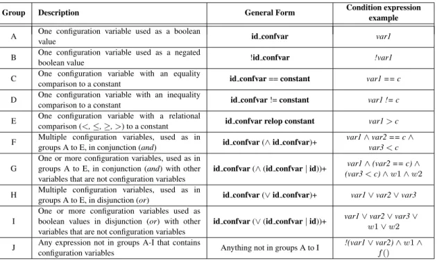
In order to divide the problem of analyzing control statements, our approach divides condition expressions into ten different groups, labeled A to J. Table I gives a short description, a general form
Table I. Description of control statements groups
Group Description General Form Condition expression example A One configuration variable used as a boolean
value id confvar var1
B One configuration variable used as a negated
boolean value !id confvar !var1
C One configuration variable with an equality
comparison to a constant id confvar == constant var1 == c D One configuration variable with an inequality
comparison to a constant id confvar != constant var1 != c E One configuration variable with a relational
comparison (<, ≤, ≥, >) to a constant id confvar relop constant var1> c F Multiple configuration variables, used as in
groups A to E, in conjunction (and) id confvar (∧ id confvar)+
var1∧ var2 == c ∧ var3< c G
One or more configuration variables, used as in groups A to E, in conjunction (and) with other variables that are not configuration variables
id confvar (∧ (id confvar | id))+ var1∧ (var2 == c) ∧ (var3< c) ∧ w1 ∧ w2 H Multiple configuration variables, used as in
groups A to E, in disjunction (or) id confvar (∨ id confvar)+ var1∨ var2 ∨ var3 I
One or more configuration variables used as boolean values in disjunction (or) with other variables that are not configuration variables
id confvar (∨ (id confvar | id))+ var1∨ var2 ∨ var3 ∨ w1 ∨ w2 J Any expression not in groups A-I that contains
configuration variables Anything not in groups A to I
!(var1∨ var2) ∧ w1 ∧ f ()
and an example statement for each group. In those examples,varxare configuration variables,cis
a constant andwxare any variables that are not configuration variables. This section will explain
how we chose to analyze statements of each group. For any given example, we will suppose that enum var is an enum variable of typeenum type with three possible values: VAL0, VAL1 and VAL2.
Groups A and B statements are analyzed quickly for boolean configuration variables and it is easy to determine which edges of the control flow will be executed for any given value of the configuration variable. In the case where configuration variables are enums, the approach remains simple, since in languages such as C, enum variables are typically evaluated to false if their associated integer value is 0 and to true for every other value. By default, the first declared constant of an enum will evaluate to false, while every other declared constant evaluates to true. For example, given a condition (enum var), we know that the condition will evaluate to false for the value enum var.VAL0, whereas it would be true for values enum var.VAL1 or enum var.VAL2.
A similar analysis can be done for groups C to E. However, in these situations, the constantcto which the configuration variable is compared must also be taken into account. For boolean variables, this constant will usually be eithertrueorf alse, while for enums, it will usually be equal to one of the possible enum values. Thus, if we have a condition (enum var != enum type.VAL1), we know that the condition will evaluate to false for the value enum var.VAL1, whereas it would be true for values enum var.VAL0 or enum var.VAL2.
Groups F and G are analyzed differently, since they are actually conjunctions of multiple conditions from groups A to E. Our strategy to analyze these conditions is to divide them into multiple subconditions. These subconditions are then necessarily either a condition that is in a group that we know how to analyze or a condition that uses a variable that is not a configuration variable. Because of the use of conjunctions, we know that if the condition evaluates to true, then each subcondition must also evaluate to true, which implies that we know the possible values of every configuration variable that makes the condition true. However, a similar conclusion cannot be made if the condition evaluates to false: in this case, the only conclusion we can draw is that each
configuration variable contained in the condition may have influenced the execution of this control flow branch.
Conditions from groups H to J are harder to analyze because of their use of disjunction or, in the case of group J, because of their overall complexity. Our analysis of those conditions simply concludes that each configuration variable contained in the condition may have influenced the execution of related control flow branches. This is conservative, since our analysis of those conditions recognizes that configuration variables may have an influence on the program control flow, but does not make any definitive conclusion during the control statements analysis.
5.3. Generate the Control Flow Graph
Generating a control flow graph for a target software program can be accomplished by parsing the program to generate an Abstract Syntax Tree (AST) for each of its source files. Navigating the AST then makes it possible to create a CFG:
CF G = (VCF G, ECF G) (2)
with multiple entry nodes vINi∈ VCF G and their corresponding exit nodes vOU Ti ∈ VCF G.
Each entry node represents a possible entry point of the system. While most computer programs have a single entry point, supporting multiple entry nodes allows our analysis to be compatible with systems having multiple entry points.
Nodes in VCF G can be of type generic, call begin or call end. Nodes of type generic are
involved in intra-procedural control flow; nodes of typescall beginandcall endare used in inter-procedural control flow, since they identify which function is called and where the function call returns in the CFG.
Edges inECF Gcan be of typegenericorgrant. Edges of typegenericrepresent intra-procedural
transfers of control that do not depend on any configuration variable; edges of typegrantrepresent intraprocedural transfers of control that depend on a non-empty finite set of properties related to configuration variables.
Edges of typegrantare created for each edgeei∈ ECF Gwhose source node is a nodevj ∈ VCF G
which represents a control statement using a configuration variable. Condition expressions found in these nodes have been analyzed as described in section 5.2. These edges are annotated with a set of properties that represent the results of the control statement analysis. For a configuration variablex used in a control statement nodevj, properties of edgeeican be of multiple types, depending on the
influence ofxover the condition. The following properties are defined: • Gain(x): if edgeeiis traversed, we know the variablexto be true;
• Loss(x): if edgeeiis traversed, we know the variablexto be false;
• SomehowPlus(x): if edgeei is traversed, it may be because of the value of the variablex
(used for the if condition true edge);
• SomehowMinus(x): if edgeeiis traversed, it may be because of the value of the variablex
(used for else statements and the if condition false edge).
Gain and loss can be determined for conditions of groups A to F, while somehowPlus and somehowMinusare used for conditions of groups G to J. SomehowMinus properties are also used for else branches of group F conditions. Even though somehowPlus and somehowMinus have similar definitions, the SomehowMinus property is necessary because of the way we later extract configuration-controlled statements using model checking, as explained in section 5.4.
Figure 4 shows a simple condition with a configuration variable config1 and its associated CFG. The CFG indicates that when the edge from the condition to b++; is traversed, the config1 configuration variable is true, thus leading to a Gain(config1) property. On the other hand, when the edge from the else to b−−;is traversed, config1 is false, leading to a loss(config1) property.
5.4. Extract Configuration-Controlled Statements
Once properties have been assigned to pertinent edges and the control flow of the system is available through the inter-procedural CFG, a model checking approach is used to determine
Figure 4. Sample Code and Extracted CFG
which statements are controlled by which configuration variables. Our methodology uses the model checking technique described in section2.2.
As stated in section 5.3, our approach defines four properties for each configuration variablexi:
gain(xi), loss(xi), somehowPlus(xi)and somehowMinus(xi). A CFG edge can grant one or more
properties and this information is available simply by taking the system CFG as input. Given a system withnconfiguration variables, results will be generated by model checking one automaton per property, so4 × nautomata. Since our goal is to locate features across the entire source code, every CFG node is converted to a state in the automaton, which means that each automaton contains 4 × ynodes, whereyis the number of nodes in the CFG.
With our model checker, four states qv,j,k are present in the automaton for each nodev in the
CF Gand for each propertyP. In this context,jis the propertyP satisfaction value of the previous calling context in the inter-procedural call graph andkis the current propertyP satisfaction value, as defined in equations 3 and 4.
rp(v, P ) =
(reachable(qv,0,0, P ), reachable(qv,1,0, P ), reachable(qv,0,1, P ), reachable(qv,1,1, P ))
(3)
reachable(qi,j,k, P ) ≡
∃p = (q0,0,0, ..., qm, qm+1, ..., qi,j,k) | qm∈ QA(qm, qm+1) ∈ TA (4)
These reachability profiles are obtained by running the model checker on an automaton that corresponds exactly to the CFG extracted from the source code. For any edgeeof the automaton, e.grantrepresents the set of properties that are granted by edgee. Equations 5 to 8 link each possible state to the original CFG.
CF G = (V, E) v ∈ V, e ∈ E reachable(qv,0,0, P ) ↔ ∃p = (q0,0,0, ..., qm, qm+1, ..., qv,0,0)@e = (qm, qm+1) | P ∈ e.grant (5) reachable(qv,1,0, P )
T his state is not possible f or our input CF G (6)
CF G = (V, E) v ∈ V, e ∈ E reachable(qv,0,1, P ) ↔
∃p = (q0,0,0, ..., qm, qm+1, ..., qv,0,1)∃e = (qm, qm+1) | P ∈ e.grant
CF G = (V, E) v ∈ V, e ∈ E reachable(qv,1,1, P ) ↔
∃p = (q0,0,0, ..., qm, qm+1, ..., qv,0,1, qv,1,1)∃e = (qm, qm+1) | P ∈ e.grant
(8)
Temporal logic predicates onvand P can be re-stated in terms of temporal logic predicates of automata states and, in turn, on reachability profiles as follows:
def+(P, v) ≡2(q v,0,1∨ qv,1,1) (9) CF G = (V, E) v ∈ V def+(P, v) ≡ ∀p = (v 0, · · · , v) → P ≡ (¬(reachable(qv,0,0, P ))) ∧
(¬(reachable(qv,1,0, P ))) ∧ (reachable(qv,0,1, P ) ∨ reachable(qv,1,1, P ))
(10)
For each configuration variable and each property, the model checker outputs the reachable states in the corresponding automaton. Unreachable states do not appear in the results files. Resolving equation 10 is thus a simple matter of observing the reachable states in the corresponding results file.
The use of model checking to propagate properties and eventually locate functionalities in the source code has some limitations. Since each configuration variable has four properties, results for each property must be merged together so that conclusions can be made about the influence of the variable on each CFG node. Moreover, since configuration variables are analyzed independently from one another, results must be merged if multiple variables are to be considered together when locating features. For those reasons, some post-processing must be applied to model checking results to map features to source code.
5.5. Mapping Features to Source Code
While the model checking results provide the reachability profile of the four properties of each configuration variable, these raw results need to be interpreted so that features can be mapped to their related source code. For program comprehension purposes, CFG nodes can be classified according to the influence a nonempty arbitrary set of configuration variables X has on their execution. Discussions with our industrial partners led us to classify each CFG node into one of the following six categories:
• Unreachable: the node is not encountered in the model checking;
• Common: the node is always executed regardless of the values of the configuration variables inX;
• Necessary: the node is executed specifically because of the values of the configuration variables inX;
• Maybe: the node may be executed because of the values of the configuration variables inX; • Not: the node is not executed specifically because of the values of the configuration variables
inX;
• DeadCode: the node cannot be executed in the software.
5.5.1. Results Merging for One Variable
Since the model checking tool analyzes each of the configuration variables separately, two merging steps are necessary to correctly extract the code related to multiple features. We first need to classify each CFG node according to the results for a single configuration variable. Once this has been determined for each requested configuration variable, the results for each variable need to be merged.
This merging needs to be conservative, in the sense that it is preferable to identify unnecessary code for a feature than to lack necessary code. Thus, all our merging needs to take into account the fact that all CFG nodes whose execution is influenced by a configuration variable must be identified. This implies that a CFG node can only be rejected from being influenced by a variable if it is definitely not influenced.
For a single configuration variable, each CFG node can be classified in a category according to the reachability profile of its four properties. This can be done by applying boolean formulas on the possible reachabilities of a CFG node. Since the model checking is done independently for each configuration variable, we first need to determine the category of each CFG node for each configuration variable. For every possible category, an equation can be applied to classify each CFG nodevi, for each configuration variablexj.
The unreachable category is used to indicate that a node has not been encountered during model checking. This is usually because the node is not part of a function, such as a global variable declaration, or because it is only being called through function pointers, which we do not currently resolve. We can easily detect these nodes because the model checker does not reach them. Thus, any node that is not reachable is consideredunreachable.
The common category represents code that is executed without any influence from the configuration variable. Logically, any CFG node that can be reached without any activated property is common. Moreover, any node that cannot be reached definitely with any of the four properties is also common, since this implies that it is possible to execute the node without any influence from configuration variables.
Common(xi, vj) = ¬def+(Gain(xi), vj) ∧ ¬def+(Loss(xi), vj) ∧
¬def+(SomehowP lus(x
i), vj) ∧ ¬def+(SomehowM inus(xi), vj)
(11) The necessary category is used for code that is necessary because of the value of the configuration variable. Since we want our analysis to be conservative, nodes that can be classified in this category are those that are definitely reached with a gain property while not being definitely reached with a loss property.
N ecessary(xi, vj) = def+(Gain(xi), vj) ∧ ¬def+(Loss(xi), vj) (12)
The maybe category is used for CFG nodes whose execution may or may not be influenced by the configuration variable. Since some conditions are very complex, it is hard to analyze their impact on the program flow. Thus, these conditions lead to the SomehowPlus and SomehowMinus properties which are used to characterize this uncertainty. A CFG node can be classified as maybe if it is definitely reached with a somehowPlus or somehowMinus property. However, it must not also be definitely reached by a gain or a loss (which would classify it in the necessary or not categories, respectively).
M aybe(xi, vj) = (def+(SomehowP lus(xi), vj) ∨ def+(SomehowM inus(xi), vj)) ∧
¬def+(Gain(xi), vj) ∧ ¬def+(Loss(xi), vj)
(13) The not category is used for code that is not necessary because of the value of the configuration variable. Since our analysis is conservative, nodes that can be classified in this category are those that are definitely reached with a loss property while not being definitely reached with a gain property. Since those nodes are only reachable without the activated configuration variable, we can safely assume that they are not used for the implementation of the associated feature.
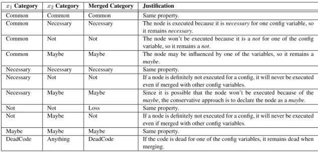
Table II. Conservative category merging table for multiple variables
x1Category x2Category Merged Category Justification
Common Common Common Same property.
Common Necessary Necessary The node is executed because it is necessary for one config variable, so it remains necessary.
Common Not Not The node won’t be executed because it is a not for one of the config variable, so it remains a not.
Common Maybe Maybe The node may be influenced by one of the variables, so it remains a maybe.
Necessary Necessary Necessary Same property.
Necessary Not Not If a node is definitely not executed for a config, it will never be executed even if merged with other config variables.
Necessary Maybe Maybe Since it is possible that the node won’t be executed because of the maybe, the conservative approach is to declare the node as a maybe. Not Not Loss Same property.
Not Maybe Not If a node is definitely not executed for a config, it will never be executed even if merged with other config variables.
Maybe Maybe Maybe Same property.
DeadCode Anything DeadCode If the code is dead for one of the config variables, it remains dead when merging.
The dead code category represents code that can’t be executed. This happens when a node can be definitely reached with a gain and a loss at the same time. In theory, it should never happen in avionics software, since avionics code can’t contain dead code.
DeadCode(xi, vj) = def+(Gain(xi), vj) ∧ def+(Loss(xi), vj) (15)
It is important to note that a nodevjcan only be classified in one category for each configuration
variablexi. Appendix 9 shows the full truth table of the four properties and their associated category.
5.5.2. Results Merging for Multiple Variables
Once each CFG node has been classified for one configuration variable, we need to merge resulting categories for each node with the categories obtained for other configuration variables. This merge needs to be conservative so that we don’t lose code that could be necessary to the set of selected features. Table II shows how this merging can be done for two configuration variables, with a textual justification for each merge.
LetX be the set of configurable variables to merge for a specific CFG nodev: equations 16 to 20 explain what each classification means for multiple variables.
Common(X, v) ↔ ∀x ∈ X | Common(x, v) (16)
N ecessary(X, v) ↔ ∃x ∈ X, ∀y ∈ {X \ x} |
N ecessary(x, v) ∧ (N ecessary(y, v) ∨ Common(y, v)) (17)
N ot(X, v) ↔ ∃x ∈ X, ∀y ∈ {X \ x} | N ot(x, v) ∧ ¬DeadCode(y, v) (18)
M aybe(X, v) ↔ ∃x ∈ X, ∀y ∈ {X \ x} |
Figure 5. Results report and related HTML file for the analysis of the config.config1 configuration variable
DeadCode(X, v) ↔ ∃x ∈ X | DeadCode(x, v) (20)
By applying those equations, we can classify each CFG node for any set of configuration variables. Since we can link CFG nodes to the source code they represent, this makes it possible to easily map features to their related source code. For any featurefrelated to a configuration variable, the CFG nodes that implement it are either classified in thenecessaryor themaybecategories.
5.5.3. Results Visualization
In order to allow users to locate their desired features easily, we developed a small GUI through which the user can select configuration variables and then calculate their results. Results are generated in HTML format, with lines highlighted in a specific color that corresponds to the category of their related CFG node. One HTML file is generated for each file of the source code.
Once results for selected configuration variables have been generated successfully, a results report is presented to the user. This report consists of a list of code blocks that are in the necessary, maybe,notanddeadCodecategories. A code block consists of consecutive lines of code that are in the same category. For each identified code block, its size and its location is shown to the user. For any set of selected configuration variables, this report makes it simple to quickly identify which files implement the desired feature and then locate pertinent lines of code using the highlighting in the generated HTML files.
A major advantage of using code blocks is that our feature mapping is done at statement granularity. Figure 5 gives an example of a results report and its related HTML file for the analysis of the aircraft type.ROTOR configuration variable. The example is synthetized because of the sensitive nature of the avionics domain. This report indicates that three code blocks have been classified in the necessarycategory for this variable. The code related to one of these blocks is shown highlighted in green, while the code highlighted in blue is code that was classified in thecommoncategory and the code highlighted in red is in thenotcategory.
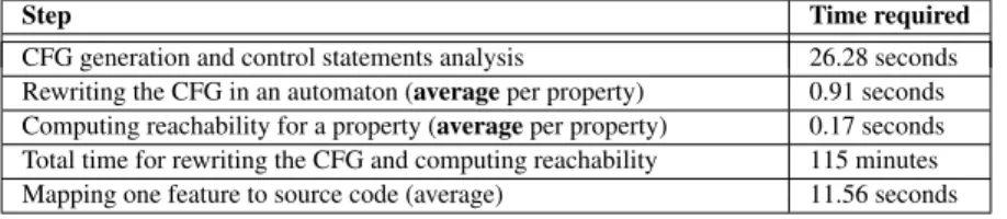
Table III. Performance of the approach for the FMS
Step Time required
CFG generation and control statements analysis 26.28 seconds Rewriting the CFG in an automaton (average per property) 0.91 seconds Computing reachability for a property (average per property) 0.17 seconds Total time for rewriting the CFG and computing reachability 115 minutes Mapping one feature to source code (average) 11.56 seconds
6. EXPERIMENTATION AND RESULTS 6.1. System Under Study
Our research is done in collaboration with a consortium that includes three companies from the avionics industry. It is part of a project to reduce the costs of certified avionics software by using model-driven development and formal methods. Mapping features to software is the first step of this project, our goal being to use the resulting knowledge to reengineer the system under study and build models for this system.
We evaluated our feature location methodology on an industrial avionics system provided by one of our partners. The system is a Flight Management System (FMS) that has been in development for 15 years and is currently used in four different types of aircraft. It is almost entirely written in C. The actual FMS resulted from the reengineering of a legacy system entirely written in assembly code and parts of the FMS still contain assembly code. It contains more than a half a million LOCs distributed over a thousand files and functions.
Since the system under study is an avionics system, it must comply with multiple standards and it has some particularities, as described previously in section 3.2. Multiple software tests are available for the system since full statement coverage is required for software to be deployed on an aircraft. However, testing the FMS takes a signficant amount of time and money, which means that existing dynamic feature location approaches are costly to apply. Thus, a less expensive feature location technique is of interest for embedded software such as the one under study.
6.2. Applying the Methodology
The approach proposed in this paper was evaluated on the FMS. Table III gives the time required to apply our methodology to the FMS system on a Intel Core I7 930 with 6 GB of RAM. While the model checking step takes about two hours (115 minutes) to compute, it is important to note that it only needs to be computed once. Once results from model checking are available, it only takes a few seconds to map any set of configuration variables to source code.
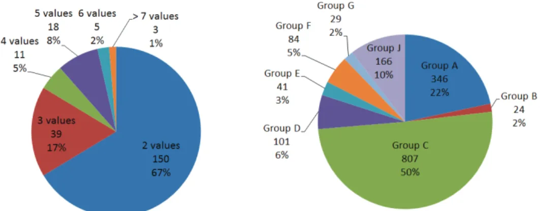
For the FMS, configuration variables were obtained by consulting its documentation, which contained a list of enum variables and indicated that they were all located in a C data structure containing hundreds of enum variables, each of which defines a certain number of constant enum values. Figure 6a gives the distribution of the number of enum values defined for each of the 226 variables of the FMS. A total of 629 enum values are defined for the FMS enum variables. It is interesting to note that most of the enum variables can take only two possible values, which means they are basically used as a substitute for a boolean. This design choice was most likely made so that each configuration variable could be used in a similar fashion. Since the identified variables were of type enum, they were converted to multiple boolean variables as described in section 5.1. Each of the obtained boolean variables is considered as a configuration variable, which means that our analysis takes into account a total of 629 configuration variables.
Analysis of the FMS showed that of all the control statements using configuration variables, 99% of them are if statement, with the remaining 1% being switch statements. This is not surprising considering that branching statements such as if and switch are necessary to control whether the code for a feature is executed or not.
(a) Distribution of the number of enum values for the 226 enum variables for the FMS
(b) Distribution of control statement groups in the FMS
Figure 6. Distribution of (a) enum values and (b) control statements groups in the FMS
Table IV. Details on the Extracted CFG for the FMS
# of nodes 372 674 # of edges 365 093 # of grant edges 3248 # of gain properties 3281 # of loss properties 3720 # of somehowPlus properties 4310 # of somehowMinus properties 2023
As shown in Figure 6b, about 82% of the conditions in the FMS are in groups A to E. As explained in subsection 5.2, these conditions contain only one configuration variable, which makes them easy to analyze. About 7% of the conditions are part of groups F and G, which we are able to analyze with full precision for thetrueedge of the condition. No condition expressions from groups H and I were found. Thus, for the entire FMS, the only conditions for which our analysis is uncertain, which eventually leads to themaybecategory, are thef alseedges of conditions from groups F-G and the conditions from group K. This means that more than 82% of the conditions of the FMS are analyzed with full precision.
For the FMS, a CFG was generated for each source file. Table IV gives some details about the extracted CFG. This CFG is used as an input to the model checking approach. Since the FMS contains 629 configuration variables with four properties each, our results are derived from model checking 2436 automata. As our goal is to locate features across the entire source code, every CFG node is converted to a node in the automaton, which means that each automaton contains 372 674 nodes. Once model checking is completed, results are available through the GUI presented in section 5.5.3.
6.3. Results
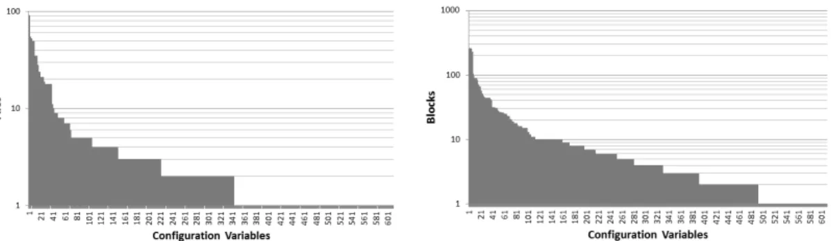
Results were calculated individually for each of the 629 configuration variables found in the FMS. The graphs in Figures 7a, 7b and 7c present the number of files, code blocks and LOCs influenced by each configuration variable, and thus by each feature, of the FMS. On average, it was found that a single configuration variable influences the execution of about 420 LOCs, across 12 code blocks and 4 files.
The two most influential configuration variables control the execution of about 36500 LOCs, across 232 code blocks and 92 files. Experts of the FMS confirmed that these two configuration variables are related to a high-level feature which controls multiple sub-features: this explains the
(a) Number of files influenced per configuration variable (b) Number of code blocks influenced per configuration variable
(c) Number of LOCs influenced per configuration variable
Figure 7. Distribution of (a) files, (b) code blocks and (c) LOCs influenced per configuration variable
large amount of code they control. It is likely that a lot of features are dependent on this high-level feature.
7. DISCUSSION
Our research shows that for dynamically configured software, mapping features to source code using static analysis is feasible. Our methodology has been assessed on an industrial avionics system and takes only a few hours to automatically match dynamically configured features to their related source code. The only step of our approach whose execution requires more than a few seconds is the model checking analysis. Thus, after the model checker has been executed once for one version of a software, our approach can map any given set of features to its related source code in a matter of seconds.
For the system under study, the FMS, it was found that 50 configuration variables influence more than a thousand LOCs each. Moreover, 43 configuration variables control the execution of code found in more than 10 files, with 25 of those variables related to more than 20 files. This shows that some features are very complex, given that they are implemented across more than a thousand lines of code and ten different files. As for code blocks, 72 features are implemented across more than 20 different code blocks. The repartition of the implementation of some features makes them hard to locate without an in-depth knowledge of the system. This justifies our feature location technique as it can be especially helpful for reengineering tasks related to those features.
Results also show that 418 configuration variables influence less than 50 LOCs. Moreover, 388 configuration variables control the execution of code found in less than 3 files, with 266 of those variables being limited to a single file. As for code blocks, 218 features are implemented in only one or two code blocks. This leads us to believe that some features have a relatively simple
implementation which is concentrated in a few code blocks and files. Considering that simpler tools could be able to locate those features, locating them with our approach might not be as helpful as locating more complex ones. However, it could be argued that our feature location technique allows a programmer with no prior knowledge of the software to quickly locate those features, which can be a significant advantage for program comprehension.
While mapping features, statements in themaybecategory are identified as being potentially part of a feature’s implementation. Statements are classified in this category because the conditions that control their execution are complex to analyze statically. Thus, we chose to identify these statements as potentially executed and leave it to the user to decide whether they are pertinent for a specified set of features. This choice was made so that our feature mapping remains conservative: some identified code may not be related to a feature, but all the code related to a feature is identified. This imprecision could be lessened by improving the analysis of control statements.
Many existing feature mapping approaches in the literature use a combination of static and dynamic analysis by combining IR and execution traces of test scenarios. Running tests can be very expensive for some software. This is especially true in the case of embedded and avionics systems, for which running test scenarios can be complex because of limited resources and timing issues. Our approach offers a less expensive approach to feature location. Moreover, given that parsers are available for many programming languages, the effort required to analyze a significant system is relatively low since our technique is entirely automated.
Using IR approaches on some systems can also give unreliable results, since the granularity of IR methods in published literature is usually at function level. This means that features implemented in specific sections of a function would not be mapped precisely. For legacy systems in which functions can sometimes have thousands of lines of code, this imprecision can be problematic. The granularity of our approach is at statement level: this allows us to locate features precisely among the source code.
We believe the approach presented in this paper is useful and easy to apply for most dynamically configured software systems. While in many cases dynamic or mixed approaches can give better results than a fully static approach, our technique has the advantage of giving results with minimal effort and expense by using only the source code as input. Moreover, it can be used in situations where dynamic approaches cannot be used because of the effort required.
Applying our feature location technique to a real avionic system, the FMS, gave us some interesting information about the system. Our interprocedural analysis revealed that features were rarely implemented at function level, but rather were spread across multiple sections of functions. Some features were also implemented across multiple, seemingly unrelated files, which validates that a feature location technique can be useful for developers to efficiently locate where features are implemented.
7.1. Limitations
The main limitation of the feature location technique presented here is that our analysis is based on evaluating the influence of software variables on control statements. This implies that only features for which execution is controlled by a configuration variable, as found in dynamically configured software, can be located. To locate features that are always active in a software program, other approaches such as the ones based on IR would be needed.
The maybe category in which some CFG nodes are classified is another limitation of our approach. This is caused by our analysis of boolean conditions found in control statements. Preferably, the condition analysis should be improved in order to minimize the amount of somehowPlusand somehowMinus properties assigned to configuration variables.
The way model checking is used in our methodology could also be seen as a limitation. Since we do not do a power set analysis of configuration variables, our approach does not consider the dependencies between the configuration variables during our analysis. Unfortunately, because of the state explosion problem and the amount of configuration variables contained in a software system, a power set analysis is not possible. For that reason, we propose a fast and feasible solution
that analyzes each property of each variable independently, which forces us to merge those results together.
7.2. Threats to Validity
For our study, there are three primary sources of threat to the validity of the results: construct validity, internal validity and external validity.
Threats to construct validity concern the extent to which the methodology measures what was intended. In our case, the threat comes from three main sources.
The proposed approach considers all features to be independent from one another. Since the analysis is done independently for each feature, our approach cannot detect and consider dependencies between configuration variables. Our GUI allows the user to select his desired configuration variables, but there is currently no consideration of possible relationship between features. For example, there is no indication that two features must never be activated at the same time, or that two features are codependent.
The system we analyzed has some functions called dynamically through constant function pointers. However, they are all part of the UI and could be ignored in our case, since our industrial partners determined the UI was irrelevant for their reengineering objectives. Analyzing a system that contains function pointers would require determining which functions each function pointer can possibly call. For constant function pointers, this can be determined by analyzing the source code. However, if function pointers are not constant, pointer analysis techniques [30, 31] would have to be used.
Our current analysis does not consider assignments of configuration variables to other variables that are not configuration variables. For the system under study, those occurrences are currently ignored, which implies that it is possible that some conditions that use configuration variables indirectly were not analyzed. This could result in incomplete feature mapping for some features of the system. The use of slicing and flow analysis could be used to resolve this issue.
Threats to internal validity concern the extent to which conclusions about causal relationships can be made. These threats usually appear when the independent variable, in our case the features of the software, is manipulated.The internal validity of our study is not threatened because we have not manipulated the independent variable.
Threats to external validity concern the extent to which our results can be generalized. So far, our approach has only been evaluated on one large industrial system written in C. Though we were able to successfully map features to the code implementing them for this system, we cannot generalize our findings for more systems. Moreover, the entire methodology has not been assessed for other programming languages.
7.3. Future Work
Future work will focus on improving the precision of our results by extending our methodology. It would be possible to improve our condition analysis by subdividing complex control statement expressions into more groups, thus allowing for a more precise analysis of these expressions. The use of pointer analysis to consider function pointers would also allow our interprocedural analysis to cover entire software systems. Another possible improvement would be to use slicing and flow analysis to consider assignments of configuration variables to other variables during our analysis.
Analyzing the interdependencies between configuration variables, and thus features, would also be very interesting for program comprehension purposes. Results from our model checker contain the necessary information to assess the dependencies between variables. However, obtaining the interdependencies would require assessing each possible combination of variables, which is hardly feasible because of the amount of configuration variables found in dynamically configured software. Future work could include interpreting those model checking results to obtain pertinent interdependencies between features.
Our approach currently uses variables to distinguish among features. Future work will extend our feature location technique by using configuration patterns to distinguish among features, with variables being the simplest configuration patterns. Configuration patterns could include function
calls and aspects, for example. Such an extension would allow our static analysis approach to be applicable to more systems.
Evaluating our methodology on other dynamically configured software is also of interest, as is comparing our static analysis feature location technique with dynamic analysis and IR-based approaches. Combining our approach with others could also lead to some novel ideas for feature location.
8. CONCLUSION
In this paper, we have presented a new approach to locate features in dynamically configured software using static analysis and model checking. We evaluated our technique on an industrial Flight Management System written in C.
The control statements of the FMS using configuration variables were analyzed and an annotated inter-procedural CFG was generated using a C parser. Model checking automata, four for each of the 629 configuration variables, were generated from the CFG. Model checking results for each automaton were then merged to locate the features related to each configuration variable in the source code.
Our technique was able to correctly locate features in the FMS. Moreover, we evaluated the distribution of features across the source code. While most features are typically located in a few files, it was found that some are distributed among a very large part of the system. We observed that 50 features are implemented with more than a thousand LOCs, whereas 25 features are implemented across more than 20 different files.
The repartition of some features of the FMS leads us to believe that our feature location approach is helpful for program comprehension. This is especially true for legacy avionics systems such as the FMS since their size and complexity can make them hard to comprehend. Better program comprehension can also be of great help for reengineering purposes, which is one of the objectives of our research project.
Future work will focus on improving the methodology to obtain more precise results. Analyzing the interdependencies between configuration variables based on our model checking results would also be very interesting for program comprehension purposes. While most existing work on feature location in the literature has focused on dynamic approaches, we believe that in some cases, feature location techniques based on static analysis are of interest for software maintenance and evolution because of their execution speed and affordability.
ACKNOWLEDGEMENTS
This project has been funded in part by the Natural Sciences and Engineering Research Council of Canada (NSERC), the Consortium for Research and Innovation in Aerospace in Quebec (CRIAQ) and our industrial partners.
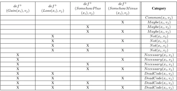
9. APPENDIX: TRUTH TABLE FOR CLASSIFYING CFG NODES
Table V shows the full truth table that can be obtained by applying equations 11 to 15 on the reachability profile of each of the four properties.
Table V. Truth Table for Equations 11 to 15
def+ (Gain(xi), vj) def+ (Loss(xi), vj) def+ (SomehowP lus (xi), vj) def+ (SomehowM inus (xi), vj) Category Common(xi, vj) X M aybe(xi, vj) X M aybe(xi, vj) X X M aybe(xi, vj) X N ot(xi, vj) X X N ot(xi, vj) X X N ot(xi, vj) X X X N ot(xi, vj) X N ecessary(xi, vj) X X N ecessary(xi, vj) X X N ecessary(xi, vj) X X X N ecessary(xi, vj) X X DeadCode(xi, vj) X X X DeadCode(xi, vj) X X X DeadCode(xi, vj) X X X X DeadCode(xi, vj)