Central bank liquidity and market liquidity: the role of collateral provision on the French government debt securities market

DOCUMENT

DE TRAVAIL

N° 278

CENTRAL BANK LIQUIDITY AND MARKET LIQUIDITY:

THE ROLE OF COLLATERAL PROVISION

ON THE FRENCH GOVERNMENT

DEBT SECURITIES MARKET

Sanvi Avouyi-Dovi and Julien Idier

DIRECTION GÉNÉRALE DES ÉTUDES ET DES RELATIONS INTERNATIONALES

CENTRAL BANK LIQUIDITY AND MARKET LIQUIDITY:

THE ROLE OF COLLATERAL PROVISION

ON THE FRENCH GOVERNMENT

DEBT SECURITIES MARKET

Sanvi Avouyi-Dovi and Julien Idier

January 2010

Les Documents de travail reflètent les idées personnelles de leurs auteurs et n'expriment pas nécessairement la position de la Banque de France. Ce document est disponible sur le site internet de la Banque de France «

www.banque-france.fr

Central bank liquidity and market liquidity:

the role of collateral provision on the French

government debt securities market

Banque de France, Paris-Dauphine University and

Julien Idier1 2

Banque de France, Paris 1 Panthéon Sorbonne University

Version: January 2010

1_{Corresponding author: julien.idier@banque-france.fr. The opinions expressed herein a those of the authors and} cannot be attributed to the institutions they are affiliated with.

2_{For insightful comments and suggestions, we are indebted to two anonymous referees, Serge Darolles, Jean-Paul} Renne, participants in the Banque de France seminar and the European Economic Association. We also thank Virginie Fajon, Guillaume Retout, Simon Strachan and Aurélie Touchais for their wonderful assistance.

Abstract:we examine the effects of collateral provision as a potential channel between funding liquidity tensions and the scarcity of market liquidity. This channel consists in transferring the credit risk associated with refinancing operations between financial institutions to market participants that bear new liquidity risk on the market associated with collateral. In particular, we address the issue of the liquidity of the French government debt securities market, since these assets are used as collateral both in the open market operations of the ECB and on the interbank market. We use a time-varying transition probability (TVTP) VAR model considering both the monetary policy cycle and the cycle of French treasury auctions. We highlight the existence of a specific regime in which monetary policy neutrality is not verified on the market for French bonds. Moreover, the existence of conventional and unconventional regimes leads to asymmetries in monetary policy implementation.

Key Words: Monetary policy, collateral, liquidity, volatility, French bond market.

Subject Classification:G10, C22, C53.

Résumé :nous considérons les effets des provisions de collatéral comme un canal de transmission entre la liquidité du refinancement et l’assèchement de la liquidité de marché. Ce canal consiste en un transfert du risque de crédit associé aux opérations de refinancement des institutions financières vers les participants de marché qui supportent alors un nouveau risque de liquidité sur le marché associé au col-latéral. En particulier, nous prenons le cas du marché des bons d’États français, étant donné l’utilisation de ces actifs à la fois dans les opérations de refinancement de la BCE et sur le marché interbancaire. Nous utilisons un modèle VAR avec changement de régimes à probabilités de transition variables dans le temps (TVTP-VAR) en contrôlant pour le cycle de politique monétaire et le cycle d’adjudication de titres d’État français. Nous mettons en évidence l’existence d’un régime particulier pour lequel la neu-tralité de la politique monétaire n’est pas vérifiée sur les marchés des titres d’États français. De plus, l’existence des régimes conventionnel et non conventionnel implique une implémentation asymétrique de la politique monétaire.

Mots-clés: Politique monétaire, collatéral, liquidité, volatilité, Marché français des titres d’États. Classification: G10, C22, C53.

1. INTRODUCTION

This paper provides an empirical analysis of the impact of funding tensions on the inter-bank market and monetary policy on a market associated with the collateral mobilized for these operations: the French government debt securities market. This asset class is used both during the open market operations (OMOs) managed by the central bank and on the secured interbank market. As in any credit operation, open market operations and the interbank fund-ing process are subject to credit risk (Stiglitz and Weiss, 1981), so that collateral is provided to ensure the lender against any default by the borrower.

Regarding the refinancing process operated by the central bank, the collateral require-ments are essential for several reasons. Firstly, they concern marketable assets usually marked to market on a daily basis. Indeed, the value of collateral is provided by the market so that it is not constant throughout the duration of the loan. This does not expose the central bank to credit risk, but to market risk. One way to circumvent this problem is the mechanism im-plemented known as variation margins: if the value of the collateral varies, banks should compensate for potential losses.

If market risk is taken into account, market liquidity becomes a key factor in determining the value of collateral (Manning and Willison, 2006). Market liquidity is the ability to obtain a fair price for an asset given that enough agents are participating in market. It has been widely studied in the microstructure literature through spread measures, resilience, transaction costs, etc. (Amihud and Mendelson, 1992; Huang and Stoll, 1997; Biais et al., 2005).

The question is whether tensions in the refinancing process of the banking system may turn credit risk into market liquidity risk via the extensive use of some types of collateral. For example, Green (2005) shows that the assets eligible as collateral provide lower rates of return than those not eligible by incurring an opportunity cost to owners. A potential risk to under-score in this paper is that the excessive use of an asset as collateral that is marked to market may ultimately create market inefficiencies. Through this mechanism, the increased credit

risk in the funding process is no longer borne by the lender but by all market participants. This transfer of risk may come from various sources.

First, the increased risk associated with interbank refinancing may create a concentration on some types of eligible collateral, i.e. those of highest quality such as government bonds. Second, this higher counterparty risk increases the haircuts on the value of the collateral so that larger amounts of collateral become necessary for the loan. Third, increased refinancing via the central bank raises the amount of collateral required. Fourth, the stepping-up of special refinancing operations, illustrating the tensions in the banking sector, results in more frequent aggressive trading of collateral. Finally, the longer maturities of refinancing operations also require larger amounts of collateral to provide to the lender. For example, in 2006, deposit collateral amounted to EUR 959 billion, while in September 2008 it stood at EUR 1,585 billion. It should be noted that this channel is identified by Brunnermeier and Pedersen (2009), who show that haircut spirals in the funding process may destabilize the entire financial sys-tem and impact the value of the collateral itself. It was a concern of the ECB monetary policy framework right from the start not to impact other financial markets, such as government bond markets, too much and to remain neutral. For example, the choice to adopt a broad approach for types of collateral instead of a narrow one, as in the case of US Federal Reserve, is understandable, as mentioned by Cheun et al. (2009), since in the US the ratio of temporary operations to the size of the domestic government bond market before the crisis was 1/200, compared to 1/10 for the Eurosystem, which would lead to substantial constraints on collat-eral and have an impact on government bond markets. In the case of the Bank of England, this ratio is 1/9, which constituted a strong incentive to expand eligibility to include all euro area government bonds (with the presence of a rating threshold). However, given the particular circumstances prevailing since the onset of the crisis in 2008, and even if the collateral ap-proach of the ECB was already broad, we wonder if market neutrality can always be achieved in the monetary policy stance.

liq-uidity of Treasury bonds and market volatility. They conclude that EMU led to sharp falls in volatility and improved efficiency in the Spanish Treasury bond market. Fleming (2003) and Goldreich et al. (2005) focus on the liquidity of US Treasuries and its impact on rates. Chakravarty and Saskar (1999) also compare the different bond segments in terms of bid-ask spreads. Moreover, Dunne et al. (2002) and Dunne et al. (2007) show that, contrary to the prevailing market belief, the 10-year segment of the French bond market is a benchmark asset for the European bond market as a whole. In addition, this market has clearly developed over the last ten years to become an important market with international investors. In our analysis, we focus on the French debt market, which is used both by banks as collateral in open mar-ket operations and on the interbank marmar-ket. Our approach is different from the papers cited above since we focus particularly on bonds as collateral, liquidity at the transaction level and the associated market risk using high-frequency data.

To analyze the role of collateral rules, we use two different maturities for French govern-ment securities: the rate on three-month Treasuries and the rate of 10-year notes. The analysis is based on high-frequency data identifying all quotations for on-the-run three-month and 10-year securities between 2003 and 2009. We analyze the impact of collateral provision on the market via the associated liquidity (bid-ask spreads) and realized volatility (specifically bipower variations from Barndorff-Nielsen and Shephard, 2003). We consider both fixed transition probabilities Markov switching vector autoregressive models (FTP-MSVAR) and time-varying transition probabilities Markov switching vector autoregressive models (TVTP-MSVAR) as in Krolzig, 1997; Filardo and Gordon, 1998 or Kim et al., 2008. TVTP-VAR models, in particular, allow for an explicit control of variables governing the regimes identified in the models. In our case, the transition probabilities are governed by both the cycle in monetary policy operations, and the cycle of French Treasury auctions of 10-year notes and three-month bills.

The main results are as follows. First, the stepping-up of special refinancing operations with high bid-to-cover ratios make more probable the appearance of an unconventional regime

in which liquidity, volatility and market segmentation between bonds occur. This is in line with the potential excessive use of some types of collateral on account of funding tensions. Second, regime identification shows the potential asymmetry in the monetary policy stance between conventional and unconventional regimes, whereby the same decision (for example more frequent OMOs and loose liquidity provision) may have positive or negative effects de-pending on the regime markets are in. As a consequence, a regime in which non-neutrality of the monetary policy stance vis-à-vis the market for collateral is observed leads to higher associated risks in the funding process.

The paper is organized as follows. In the following section, we review the concepts of market liquidity and central bank liquidity focusing on the linkages between collateral rules and market dynamics. We present the recent developments on the French sovereign bond market, including monetary policy during the 2007-2008 crisis and the funding tensions. In the third section, we define indicators of liquidity and volatility and present the framework of the models. The fourth section discusses the empirical results and focuses on their monetary policy implications. Section 5 concludes.

2. LIQUIDITY

Liquidity is an elusive financial market concept, often used to illustrate tensions observed in the global financial system in 2007-2008. However, this word encompasses several financial and more generally economic concepts. As underlined by Nikolaou (2009), we can distinguish three types of liquidity. The first is the central bank liquidity provided through open market operations. The second is the funding liquidity defined by the BIS (2008) as the ability of banks to meet their liabilities, and unwind or settle their positions as they come due. Finally, the third type of liquidity concerns market liquidity, defined by the IMF (2004) as the ability of investors to trade quickly, at a fair price and low cost, a large amount of shares with a small impact on prices. In 2007-2008, we observed in the financial system:

a shortage of funding liquidity;

a shortage of market liquidity in the funding market;

central bank liquidity acting as a substitute for the market;

a shortage of market liquidity on some other markets.

These diverse liquidity concepts are very close to each other but the potential channels between them are not so well understood. Here we investigate the potential channel between these three liquidity concepts constituted by the rules on collateral.

2.1. Collateral provision and liquidity

The central bank provides liquidity to banks through several channels. The majority of these operations are main refinancing operations (MROs) with a weekly frequency. The cen-tral bank also uses long-term refinancing operations (LTROs), the more recent very long-term refinancing operations (VLTROs) and some other one-off fine-tuning operations (FTOs). A de-tailed description of this primary channel of central liquidity is discussed in Idier and Nardelli (2010) with a focus on the March 2004 reform of liquidity management.

A second channel for providing liquidity is the use of standing facilities. Any bank may ask the central bank for refinancing at any time at a penalty rate. This penalty is such that few banks generally use these standing facilities. There is a "standing facility stigma" since banks are usually reluctant to use them: it is usually a signal of weakness to the market for the bank using the lending facility (even if it is theoretically confidential). However, the recent crisis has shown a clear increase in the deposit facility linked to an increase in risk aversion, and a reduction of the penalty associated with it.

All these operations managed by the central bank lead to some collateral immobilization, which we focus on here. To protect the ECB (and more generally any central bank) from losses due to open market operations, collateral is used to back the operations. In the event of

credit failure, this collateral may be liquidated by the central bank to get its money back. The assets used as collateral must meet certain criteria to be eligible for the ECB in its refinancing operations (see ECB "The implementation of monetary policy in the euro area", November 2008). These rules were modified in early 2007 with the introduction of the single list of eligible assets. Notably, the ECB considers collateral eligibility for marketable and non-marketable assets.

Concerning marketable assets, euro-denominated debt instruments with high credit rat-ings traded on regulated markets3are eligible, provided that the issuer is an EU member or a G10 member. Non-marketable assets (credit claims and retail mortgage-backed debt instru-ments) must be issued by credit institutions located in the euro area, with high credit ratings and be denominated in euro. However, in the ECB’s monetary policy framework, the collat-eral policy is gencollat-erally restricted to marketable assets for outright transactions.4

To ensure the quality of collateral the ECB uses two additional measures: the haircut and variation margins. An important aspect is that the value of the asset is marked to market so that the ECB is exposed to downward variations in the collateral’s value during the loan period. As a consequence, counterparties (banks) must provide additional cash to maintain the value of the asset (margin-calls). Obviously, these variation margins are symmetrical and if the value of the asset rises above a certain level, the counterparty retrieves the corresponding cash.

The haircut is a percentage discount applied to the value of the collateral. The value of the collateral is thus calculated as the market value of the asset less the haircut applied to this category of assets.

The ECB has integrated this market dependency into its rules so that the level of the haircut is based on a liquidity criterion: the lower the liquidity, the higher the haircut. However, this criterion is quite rigid and may not completely hedge the ECB against market inefficiencies.

3_{There are some exceptions in published lists of non-regulated markets accepted by the ECB.} 4_{Some of these criteria have been relaxed during the crisis episode but for a limited period of time.}

There are five categories of liquidity for the assets used as collateral. The first category is considered to be the most liquid, with liquidity decreasing progressively across the four other categories. Table 1 sums up these categories as regards marketable assets.

Category I Category II Category III Category IV Category V

Central government debt instruments

Local and regional government debt instruments Traditional covered bank bonds Credit institution debt instruments (unsecured) Asset backed securities Debt instruments issued by CBs Jumbo covered bank bonds Debt instruments issued by corporate and other issuers Agency debt

instruments Supranational debt

instruments

Table 1: Liquidity categories for marketable assets (source: ECB)

In each of these categories, depending on the residual maturity and the coupon, the haircut varies from 0.5% to 20%. The best choice of collateral for participating to OMOs are thus the government debts instruments. They usually meet high credit standards, enjoy market liquidity and are traded on organized markets.

In addition, government bonds are also used as collateral in bilateral transactions on the interbank market to cover funding liquidity needs. Given the financial instability seen on the market during the last few months, the secured segment (on the short maturity) of the interbank market has served as a substitute for the unsecured segment due to the funding

liquidity tensions. However, turnover in this market segment has slowed (a fall of 16% in comparison with 2004-2005 levels), due to the decline in the quality of the collateral usually used in bilateral repo transactions and the uncertainty related to counterparty risk. There is therefore also a clear incentive to ask for high quality collateral on the secured market.

2.2. The implications of the crisis for liquidity

We investigate the funding liquidity pressure impact on the liquidity and volatility of as-sets used as collateral. The 2008 crisis seriously undermined the interbank market. The ECB thus decided to provide huge amounts of liquidity to the banking system through regular and special OMOs.

With respect to regular open market operations, the ECB first increased the levels of al-lotments to meet liquidity needs through MROs and LTROs. Due to the high demand for liquidity, the ECB decided to use a fixed-rate tender with full allotment in order to completely satisfy bank liquidity needs. In a fixed-rate tender, the ECB gives the level of the rate ap-plied to the MRO and banks are asked to give the corresponding amount of liquidity they are willing to obtain at this price. In this way, their needs are completely met given the level of the rate. This is in contrast to variable rate tenders in which banks provide ten rates and ten corresponding amounts of liquidity that they are willing to obtain with no guarantee of the final amount allotted. In this way, the ECB limits tensions on the interbank market, but provides large amounts of liquidity to the banking system, and this requires higher amounts of collateral. This has also been coupled with the stepping-up of special operations as shown in Figure 1.

The proportion of operations other than MROs and LTROs has dramatically increased during the recent period5from 3 to 40%. Moreover, from 2000 to July 2007 the mean amount per operation of allotted liquidity in special operations was around EUR 17 billion, versus around 40 billion between August 2007 and October 2008. Moreover, until July 2009, we note

43% 29% Feb-09 - Jul-09 40% 21% Jul-07 - Feb-09 3% 18% Jan-00 - Jun-07 43% 29% 29% Feb-09 - Jul-09 OT MRO LTRO 40% 39% 21% Jul-07 - Feb-09 OT MRO LTRO 3% 79% 18% Jan-00 - Jun-07 OT MRO LTRO

Source: ECB, authors’ calculations

FIG. 1Proportion of ECB liquidity operations by type

no return to normal of the liquidity-providing operation calendar.

On the collateral side, the ECB took several measures to ensure the soundness of open market operations in late 2008 (Directives ECB/2008/15 and ECB/2008/18). In particular, it extended eligibility (with higher haircuts) to some other asset classes (asset backed securities, syndicated loans for a given period, Japanese, US and UK credit claims, for example).

All these tensions in the banking system, resulted in the interbank market in a reluctance for banks to lend to each other. However, when bilateral transactions occur, it seems that high quality collateral is required and French government bond securities belong to this category. This is illustrated in the OIS spread (see Figure 2), closely followed by market participants during the turmoil, and reflecting the credit risk associated with transactions on the interbank market.

-0.4 0.0 0.4 0.8 1.2 1.6 2.0 2005 2006 2007 2008 2009 Source: Datastream

FIG. 2Euribor-OIS Euribor spread between 2005 and July 2009

European market as a whole, high volatility on bond yields for short and long-term maturities has been observed since August 2007. Moreover, bid-ask spreads also started to widen (see ECB Monthly Bulletin, October 2008).

Due to governments’ fiscal commitments aimed at tackling the crisis and a general rise in credit risk premia, risk aversion on bonds over the long term has increased. This is now reflected in the yields for long-term securities. However, this has not occurred for all gov-ernment bonds within the euro area. On the one hand, bonds are suffering from a flight to quality phenomenon whereby investors shift trading to traditionally strong government debt securities (typically German or French ones). On the other hand, there is also a flight to liq-uidity issues with investors wishing to invest in liquid markets. In a period where refinancing is difficult on the interbank market, it is clear that banks are mitigating their risk by investing in markets where funds may be withdrawn rapidly. As a consequence, the liquidity of some

bond markets has dried up (for example the Greek market) and trading has shifted to other bonds markets. This combination of flight to quality and flight to liquidity may have marked consequences for market efficiency.

3. AN EMPIRICAL ASSESSMENT OF THE COLLATERAL CHANNEL

3.1. Dataset and market indicators

Our dataset consists in high-frequency (on-the-run) quotes for French debt securities with 3-month and 10-year maturities from Reuters Data Tick History ranging from January 1st, 2003 to July 31st, 2009. We have around 3.5 millions quotes for the bonds in question. Some public holidays were removed from the sample due to the lack of trading (Christmas, New Year Eve, Easter, France’s national holiday, etc.). Due to the greater dispersion of 3-month contracts, with more frequent adjudications, the number of quotes is lower than for the 10Y notes, for on-the-run contracts.

3.1.1. Liquidity indicators

The bid-ask spread reflects many factors (see Roll, 1984; Glosten, 1987; Glosten and Harris, 1988, 1991; Huang and Stoll, 1997; Hasbrouck and Seppi, 2001). One main component is the transaction cost on the buy side and on the sell side. The larger the spread, the higher the transaction cost (for bond markets, see Harris and Piwowar, 2006). Assuming that the true value of the asset is in between the bid and ask prices, the larger the spread, the higher the potential gap between this true value and the price investors have to pay for buying or selling it. Fleming (2003) assesses in particular that spreads are good measures for tracking liquidity on Treasuries. This measure is used in many markets and allows for comparisons as in Chordia et al. (2003). Under usual market conditions, the price is defined as the difference between the ask price and the bid price. We construct an average daily bid-ask spread for each rate. Since we are looking at the bid-ask spread for rates, which are inversely related to

prices, the spread is defined as:

Si,t=ri,tbid raski,t (1)

for the ithtransaction of day t. The daily liquidity indicator is then the mean over the day of all spreads:6 St= 1 N N

∑

Due to the partial information available on our dataset (e.g. no details about transaction volumes), we restrict our analysis to this standard indicator as suggested by Fleming (2003).

3.1.2. Volatility measures

Since the seminal paper of Merton (1980), realized volatility has been widely used in the lit-erature. Typically, it uses the intraday returns of an asset to calculate daily volatility measures by approximation of the quadratic variation. There are several realized volatility estimators (see Avouyi-Dovi and Idier, 2010), but here the bipower variations are calculated following the work of Barndorff-Nielsen and Shephard (2003). First, let us consider a partitionΨ of the day retaining the last transaction of equal subintervals of time (one hour in our case study). Then, the day t volatility estimator is defined as:

RVt=

∑

jriri j (2)

where riand ri are subsequent returns for the considered subintervals of day t. The rationale

for this choice comes from its ability to remove the jump component. These jumps may be quite usual during the day for liquidity reasons typically. This is not the case for the standard realized volatility estimator of Merton (1980) defined as the daily sum of squared returns (see Andersen et al., 2006; Barndorff-Nielsen and Shephard, 2002; Barndorff-Nielsen et al., 2006; Huang and Tauchen, 2005; Tauchen and Zhou, 2004). The bipower variations are applied to

bond yields and computed on 15-minute-frequency returns.

3.1.3. Monetary policy and funding tension indicators

To investigate monetary policy, we construct several indicators representing the ECB’s op-erational framework and tensions during the refinancing process. First of all, we consider a set of dummy variables for OMOs, and their type: MROs, LTROs or Other. We also use the allotted amount of OMOs and the bid-to-cover ratios of these operations. This bid-to-cover ratio is the supply-demand ratio for liquidity. It summarizes some of the tensions related to refinancing between banks. All these indicators give the intensity with which market par-ticipants are seeking refinancing from the central bank and how the collateral market, as a consequence, may be impacted by these operations.

3.2. Bond market and funding liquidity tensions

The amount of the negotiable debt for the French government almost doubled between 1998 and 2008, reaching EUR 988 billion at the end of September 2008. This upward trend was made possible by the introduction of marketable products grouped into three categories based on their initial maturities. The first category comprises the short-term bond class with maturities less than one year. In this category, three-month maturity bonds are typically is-sued weekly and respond to short-term financing needs. The second category includes bonds with two or five-year maturities with a new adjudication per month. The last category con-cerns long-term bonds with maturity from seven to 50 years with one adjudication per month. After these regular pre-scheduled auctions, securities are actively traded on the secondary market, where transactions are not centralized. This secondary market is an over the counter market (OTC) and bilateral transaction details are partially known.

One main development in this market is its internationalization. An increasing share of the negotiable French debt is held by foreign investors : by the end of 1998, it represented

18.8% of negotiable debt compared with 62% by mid-2008. This internationalization could be a vector of increasing liquidity on the market with a wider pool of market participants.

Figure 3 shows the daily changes in bond rates. While the short-term rate is anchored to changes in the minimum bid rate of the ECB, 10-year rates are more independent of the rise in interest rates that occured from the end of 2005. As a consequence, the bond spread shrank until spring 2008. From September 2008, the financial crisis and the ECB’s decision to cut interest rates clearly increased this bond rate spread, with a huge drop in short-term maturity rates (see Figure 2).

3 4 5 6 0 1 2

Jan-03 Aug-03 Mar-04 Oct-04 May-05 Dec-05 Jul-06 Feb-07 Sep-07 Apr-08 Nov-08 Jun-09 rate120 rate3

Source: Thomson Reuters Tick History, authors’ calculations

FIG. 3Daily rate for French bonds between 2003 and 2009

With respect to liquidity, Figure 4 presents the bid-ask spread for the two bonds between 2003 and July 2009. The short-term maturity bond is less liquid than the longer-term one over the sample. The average bid-ask spread for three-month maturity rates is about 3.7 bp, while

it falls by 0.8 bp for the 10-year one.7

Broadly on the sample, the bid-ask spread for short-term maturity fell except during the crisis of 2008 where it jumped twice in September and October. Moreover, volatility also surged during this period.8We note that the impact is stronger for the three-month maturity than for 10-year bonds. Indeed, volatility for long-term bonds rose but did not soar.

There are several things to investigate in this area. First, liquidity and volatility may not have the same interactions depending on the market segment. In particular, the monetary policy framework may impact these indicators, as we mentioned earlier, so that some mar-kets may be more vulnerable than others, even if they belong to the same liquidity class of collateral as defined by the ECB.

Looking at the monetary policy stance of the ECB, the duration (maturity) of OMOs have increased over the last two years (except at the end of the sample with the proliferation of special short-term maturity operations). These longer average durations result in longer im-mobilization of collateral and thus less liquidity on the market for collateral. These longer durations are coupled with the stepping-up of operations as underlined in the previous sec-tion and the increase of allotted amounts. This clearly responds to greater liquidity needs and is confirmed by the bid-to-cover ratio. In 2007, it appears that the demand for liquidity was on average 82% higher than the amount supplied and even reached 94% in 2008.

We wonder how the market for collateral is impacted by such developments in monetary policy operations, i.e. stronger competition for liquidity and an increase in allotted collateral-ized amounts.

7_{This is also confirmed by the relative bid-ask spreads.}

8_{For graphic convenience in Figure 4, three huge peaks in October 2008 (with a level of around 2800) have been} removed from the graph showing the volatility of the 3-month rate.

0.02 0.03 0.04 0.05 0.06 0.07 0.08

Bid Ask spread 10Y rates

0.1 0.2 0.3 0.4 0.5

Bid Ask spread 3M rates

0 0.01 0.02 0.03 0.04 0.05 0.06 0.07 0.08 Ja n -0 3 Ja n -0 4 Ja n -0 5 Ja n -0 6 Ja n -0 7 Ja n -0 8 Ja n -0 9

Bid Ask spread 10Y rates

0 0.1 0.2 0.3 0.4 0.5 Ja n -0 3 Ja n -0 4 Ja n -0 5 Ja n -0 6 Ja n -0 7 Ja n -0 8 Ja n -0 9

Bid Ask spread 3M rates

15 20 25 30 35 40 45 50

realized volatility 10Y rates

100 150 200 250 300 350

realized volatility 3M rates

0 5 10 15 20 25 30 35 40 45 50

Jan-03 Jan-04 Jan-05 Jan-06 Jan-07 Jan-08 Jan-09

realized volatility 10Y rates

0 50 100 150 200 250 300 350

Jan-03 Jan-04 Jan-05 Jan-06 Jan-07 Jan-08 Jan-09

realized volatility 3M rates

Source: Thomson Reuters Tick History, authors’ calculations

1.4 1.5 1.6 1.7 1.8 1.9 2

Bid to cover ratio (mean per year)

1 1.1 1.2 1.3 1.4 2003 2004 2005 2006 2007 2008 2009

Source: ECB, authors’ calculations

FIG. 5Bid-to-cover ratio for ECB OMOs

3.3. A model accounting for monetary policy cycles and bond market dynamics

3.3.1. A fixed transition probability model

We first consider a general Vector Auto-Regressive (VAR) stationary process including variables such as: the daily variation in bond yields; log realized volatility calculated on the basis of the work of Barndorff-Nielsen and Shephard (2003); bid-ask spread variations. We complete this set of variables with a monetary policy operation announcement indicator (as defined in Appendix 1).

Let consider a VAR model with P lags [VAR(P)] as :

Xt= P

∑

ΦpXt p+γOMOt+µ+εt, (3)

where Xtis the vector of variables of interest as yield variations (∆r3,t,∆r120,t), volatilities (σ3,t

OMOs announcement days and zero otherwise.

However, at daily frequency, it is hard to consider a homogeneous linear model for mar-ket dynamics. Marmar-ket dynamics are not usually linear, or even piece linear, but usually gov-erned by several coexisting regimes. In line with Hamilton’s (1994) findings, we use a Markov switching VAR to capture the dynamics of the variable of interest.9To limit the number of pa-rameters to be estimated and to circumvent identification and estimation problems, since a VAR model is estimated for each regime, we limit our analysis to two states (S=2). So, con-ditional onfXtgt=1:N, the history of past variables, we consider a two state model for st=1, 2

similar to Krolzig (1997) such that

E(Xtjst) = P

∑

with utfollows a Gaussian distribution with zero mean. Since the volatility of the rates is

not constant over the sample (as presented in Figure 5), we also consider heteroskedasticity in this MSVAR through theΣ(st)state dependent variance-covariance matrix ut. By considering

the state dependent variance, we obtain a mixture of two Gaussian distributions making it possible to replicate the skewed and leptokurtotic distribution of bond yield variations (see Idier et al., 2008).

The state process is generated by a homogeneous Markov chain with two states so that the transition probabilities are defined by:

pij =Pr(st=jjst 1 =i)with S

∑

pij=1,

for i, j= f1, 2g. In this setting, the Markov chain transition matrix T is such that: T= 2 6 4 p11 p12 p21 p22 3 7 5 .

However, the FTP-model only identifies regimes without explicitly considering the in-formation or factors leading to such regimes. For example, the transition matrix may dis-play jumps during specific days because some variables lead to greater persistence of some regimes. It thus seems more relevant to identify factors which can drive changes of the tran-sition probabilities.

3.3.2. A time-varying transition probability model

As a consequence, we also propose a time-varying transition probability model (as in Fi-lardo and Gordon, 1998) to explicitly consider both the monetary policy cycle and government debt issuing cycles. In order to ensure some good convergence properties, the complexity of this model calls for a more parsimonious model than the previous one. We thus consider the 10-year debt market and the three-month market rate separately in the following formulae:

0 B B B B B B B @ ∆r120,t ln(σ120,t) S120,t ∆r3,t 1 C C C C C C C A t = P

∑

∑

with st=1, 2 and with εtand utfollow a Gaussian distribution with zero mean and state

dependent variance-covariance matricesΣε(st) andΣu(st) respectively. Even if we have to

separate models, we consider the direct linkages between rate variations by introducing∆r3,t

in eq. 5 and∆r120,tin eq. 6.

To identify the regimes detected in the model, we consider an endogenous transition prob-ability matrix, taking into account both the monetary policy cycle and the French government bond auction cycle. The choice of these variables results from several constraints. First, the frequency of the model and the daily market dynamics approach restrict the potential for in-cluding real macroeconomic variables. Second, monetary and bond cycles, for institutional reasons, are very interesting in terms of market structure since they are highly influenced by their auction processes. Finally, given the issue of the impact of monetary policy on some alternative markets, the liquidity of the funding process on the one hand and of the bond market on the other need to be controlled for these substantial institutional features.

We thus consider both dummy variables and the bid-to-cover ratios resulting from the corresponding adjudications to disentangle two possible effects:

1. We assume that the frequency of open market operations responds to a disequilibrium in cash demand from banks and smooths funding liquidity tensions. In the same vein, the scheduled debt market cycle is assumed to provide liquidity to the corresponding bond market segment.

2. However, if the higher frequency of OMOs is associated with higher bid-to-cover ratios, these operations may have an impact on markets, especially on the market for collateral, thus revealing tensions in the funding process. For the same reasons, high bid-to-cover ratios for debt auctions may reveal excess demand for this class of assets.

m= f3; 120g: Tm(t) = 2 6 4 pm,11(t) 1 pm,22(t) 1 pm,11(t) pm,22(t) 3 7 5 (7) such that

pm,ii(t) = Φ(δi+αi.OMO(t 1) +β_i.AFTm(t 1) + λi.OMO_cover(t 1) +γ_i.AFT_coverm(t 1))

withΦ beeing the cumulative normal density function, as used in Kim et al. (2008).10

In this framework, an interesting output are the regime dependent impulse response func-tions (IRF). Here, we follow the methodology used by Ehrmann, Ellisson and Valla (2003) with the additional feature that we consider generalized impulse response functions as in Pe-saran and Shin (1998) since we do not make any assumptions about the order of the variables. All variables used in the model are stationary, the tests being reported in Appendix 2. The models’ estimates use likelihood maximization. The likelihood of this process is

l(x1...xT;Ω) = T

∑

ln(f(xtjxt 1,xt 2, ...x1)). (8)

The set of parameters Ω comprises the mean equation parameters and the parameters used for time varying transition probabilities. The Gaussian density f(xt j xt 1,xt 2, ...x1)

considers the different states of the Markov switching process as

f(xtjxt 1,xt 2, ...x1) = S

∑

f(xtjst= ¯s)Pr(st=¯sjxt 1,xt 2, ...x1)

with f(xtjst= ¯s)the density conditional on the state and Pr(st=¯sjxt 1,xt 2, ...x1)the state 10_{The results presented below are robust to some other transition probability forms (for example, a logit function),} which guarantee a well-defined likelihood function.

probabilities, elements of the(1, S)vectorΠtupdated for each date as

Πt= f

(xt) Πt 1Tm(t)

[f(xt) Πt 1Tm(t)]ι0 (9)

with * the Hadamard product, ι a(1 S)vector of ones, T the transition matrix defined in equation 7 and f(xt)the vector(1, S)with elements f(xt jst = ¯s). For the robustness checks

below, we apply likelihood based tests to compare the different models to one another.

3.3.3. Model robustness and estimates

The models are estimated between the 1st of January 2003 and the 30thof July 2009. Es-timation results are provided in Appendices 3, 4 and 5. In Appendix 3, the fixed transition probability model is presented and TVTP-VAR estimates are presented in Appendices 4 and 5. Several alternative specifications are tested. In particular we present here the different steps concerning the restricted datasets X1

t =(∆r3,t, σ3,t, S3,t,∆r120,t)and Xt2=(∆r120,t, σ120,t, S120,t,

∆r3,t). The first step was to estimate a simple stationary VAR model. The next step was to

consider Markov switching VAR models for these sets of variables, and finally consider the TVTP-VAR models as presented in equations 5 and 6.

On the basis of the estimated likelihoods, we consider Vuong’s (1989) model selection tests. Let us consider two competing models with densities f and f0given a respective set of parametersΩ and Ω0. The test is defined as

1 p TLRT(Ω; Ω 0_{) = L} T(Ω) L 0 T(Ω0) = _p1 T T

∑

such that 1 p TLRT(Ω; Ω 0_{)˜N(0, ˆσ} T).

ˆσTis the heteroskedastic and autocorrelated adjusted variance of the test defined as

ˆσT =Γ0+2 J

∑

∑

similar to a Newey West (1987) correction. The results are reported in Table 2 below.

set of variables Xt1 Xt2

VAR vs. FTP-VAR 0.90

0.996 1.010.998

FTP-VAR vs. TVTP-VAR 0.026

0.724 0.1760.987

Table 2: Vuong (1989) selection model test results, (*) means rejection of the null: "models are equivalent"

The test indicates that introducing Markov switching models always improves the fit of the models. For the TVTP models, it improves the fit for 10 year rates, while the FTP and TVTP models for the 3 month rates are only equivalent.

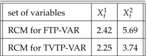
In addition, we also apply the RCM statistics from Ang and Bekeart (2002) to check if the two regimes in the TVTP-VAR models are clearly identified compared to a FTP-VAR. This statistic is defined for two states as

RCM(S) = 400 T T

∑

identification for the regimes we have.

set of variables X_t1 X2_t RCM for FTP-VAR 2.42 5.69 RCM for TVTP-VAR 2.25 3.74

Table 3: Ang and Bakeart (2002) RCM statistics for regime identification

The introduction of time varying transition proababilities improved the identification of the regimes, since we have smaller statistics in this case. Given the robustness of the TVTP-models, our comments in the following section are based on the TVTP-MSVAR models.

4. THE ASYMMETRIC IMPACT OF MONETARY POLICY

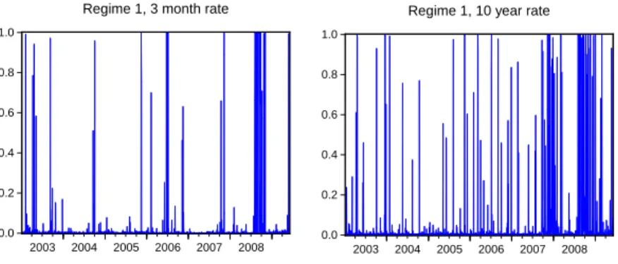
The two regimes are statistically identified and the ex-post regime probabilities are pre-sented below. The debt market cycle and monetary policy cycles help to identify two regimes, with a non standard one (regime one) which prevailed in 2007 and 2008. The unconditional transition probability in the 10-year rate model and the 3-month model are rather low in the first regime, confirming the non standard quality of regime 1.

4.1. Market inefficiencies, volatility and liquidity premia in the two regimes

The impulse response functions are obtained from the estimates of the two TVTP-MSVAR models (see Appendix 6).

In the standard regime (regime 2), rate comovements are significant and positive, both from long to short-term rates and conversely. This illustrates French sovereign bond market dynamics as whole. An initial development that appears to reveal a non standard regime on the bond market is the increasing segmentation of the bond market.

A second element is that volatility premia in the standard regime become liquidity premia, especially for the long-term rate. The liquidity premium is a factor that has proved to be of

0.0 0.2 0.4 0.6 0.8 1.0 2003 2004 2005 2006 2007 2008

Regime 1, 3 month rate

0.0 0.2 0.4 0.6 0.8 1.0 2003 2004 2005 2006 2007 2008

Regime 1, 10 year rate

0.0 0.2 0.4 0.6 0.8 1.0 2003 2004 2005 2006 2007 2008

Regime 2, 10 year rate

0.0 0.2 0.4 0.6 0.8 1.0 2003 2004 2005 2006 2007 2008

Regime 2, 3 month rate

interest in the determination of corporate and sovereign bond market dynamics (Amihud and Mendelson, 1991; Chakravarty and Saskar, 1999; Elton and Green, 1998 or Fleming and Remolona, 1999). Indeed, investors prefer to act in markets where liquidity is abundant if they are able to find a counterparty to trade the liquidation of their portfolios without incurring losses. On the treasury market, Longstaff (2002) shows some flight to liquidity phenomena in bond markets that potentially affect yield levels. Kamara (1994) and Goldstein et al. (2005) notably make the link between market transparency, liquidity and price on bond markets. Many studies have investigated the volatility and liquidity premia that interest rates may account for, such as Diaz et al. (2006) for the Spanish treasury market and Longstaff (2002) for US markets.

Figures 9 and 10 for 10-year rates show that in the standard regime there is a persistent volatility premium. This can be compared to some extent with a GARCH in mean effect with an increase in the rate stemming from a rise in volatility. This premium becomes almost in-significant in the unconventional regime with the rise of a strong and less persistent liquidity premium for the 10 year rate. In the case of the three-month segment, premia in the standard regimes are positive on prices (negative on rates). Liquidity is certainly less of a concern for investors in the three-month market, since they are closer to the liquidation of their contracts and have the option of rolling or liquidating them at a shorter horizon than for the 10-year rate.

A last noteworthy fact is the spiral between market liquidity and volatility in the two regimes (see Figures 11 and 12). Market illiquidity leads to stronger volatility for the 10 year rate and conversely, higher volatility leads to lower market liquidity. These market dynamics are reinforced in non standard regimes. This may strengthen the links mentioned in the early part of this paper. At some point in time, due to the large impact of monetary policy and tensions in the funding process, the monetary policy stance may not guarantee neutrality with respect to markets, especially the market for collateral. Via this channel, there is a regime in which funding tensions lead to market liquidity tensions when the frequency of OMOs is

high. Therefore, due to the use of this asset class as collateral, it increases the risk of some adjustments for banks exposed to collateralized credit with margin calls, since the operation itself has an impact on the market used to determine the value of the collateral. This risk is thus incompatible with the conventional monetary stance based on market neutrality.

To clarify the links between the monetary policy stance and possible market dynamics, below we discuss the impact of the monetary policy cycle in regime identification.

4.2. The role of the monetary policy cycle in regime identification

If regime 1 concerns the 2007/2008 period of turmoil, it also encompasses early 2005 and 2006, when special OMOs on the interbank market were conducted by the ECB,11and mone-tary cycles reversed in response to increases in policy interest rates.

The impact of both the frequency of OMOs and the tensions resulting from these oper-ations may be considered in different ways. On the one hand, the frequency of OMOs is sup-posed to respond to the funding needs of the banking system so that their frequency smooths possible disruptions to the financial system. On the other hand, if these operations are com-bined with a high bid-to-cover ratio, two effects may be expected: (i) a high bid-to-cover ratio may reveal the lack of funding liquidity and the fact that the ECB is not responding suffi-ciently to liquidity needs; (ii) however, it may also reveal the need for the central bank to limit its role in funding markets and to only meet efficient demand (’efficient’ would mean what is calculated as benchmark supply by the central bank), so as not to replace the interbank market.

Looking at the impact of monetary and bond cycles in these regimes (see Appendices 4 and 5), the impact of OMOs is two-fold.

In regime 2, which is the standard one, the impact of the frequency of OMOs and the bid-to-cover ratio of these operations are insignificant for the 10-year rate, thus preserving the market neutrality of monetary policy implementation. However, this is not true for the

month rate, the less liquid asset: the more frequent the OMOs, the higher the probability of switching from the standard to the non standard regime. Moreover, when the bid-to-cover ratio is low during these more frequent OMOs (i.e. the ECB largely satisfies all bids posted by banks during the auction), the persistence of the standard regime is lower. This tends to bear out the hypothesis mentioned in the early part of the paper: by stepping up OMOs and ensuring higher allotment, the central bank may be encouraging the switch from a standard regime to a non standard one by affecting the market used as collateral and triggering market inefficiencies.

However, our findings concerning the impact of monetary policy on bond market dy-namics, in the non-standard regime, indicate some asymmetric results. When this regime occurs, more frequent OMOs associated with low bid-to-cover ratios (i.e. a loose liquidity policy) appear to limit the persistence of this crisis regime.

This result is crucial since it introduces an asymmetry in the conduct of monetary policy: on the one hand, policy makers should limit OMOs and supply limited liquidity to prevent a switch from the standard to the non standard regime. On the other hand, if a crisis occurs, by stepping up OMOs and minimizing the bid-to-cover ratio of these operations, they reduce the persistence of the crisis regime.

To summarize, regime identification highlights the difficulty of managing monetary policy since identical measures may have "good" or "bad" effects depending on the regime markets are in. To limit the switch from a standard to a crisis regime, OMOs should not be stepped up and the supply of liquidity should be limited. However, to limit the persistence of the crisis regime, OMOs should be stepped up and satisfy demand for funding.

The role of the bond market cycle Bond market cycles in the endogenous transition

probability are also considered from the point of view of the frequency of bond auctions, and the tensions associated with these operations. The effects are less ambiguous for this cycle, than for the monetary policy cycle since the timetable of auctions is very rigid and does not

display any irregularity as the monetary policy cycle of OMOs may do, both in their frequency and in the auction process used.

The frequency of auctions has a homogeneous impact in the standard and in non standard regimes. When an auction is held, the persistence of the crisis regime decreases and the per-sistence of the standard regime increases for both rates. Lower bid-to-cover ratios for these operations have the positive effect of limiting the probability of a switch from the standard to the non standard regime, for both rates, and of shortening the crisis regime in the case of the three-month rate.

The importance of this regime identification process thus derives from the potential asym-metric effects of monetary policy conduct. Having reached this point, the reader may now consider the first regime as the ’unconventional’ regime, and regime two as the’conventional one’, with the less desirable fact that during the ’unconventional’ regime, the neutrality of the monetary policy stance is not guaranteed.

5. CONCLUSIONS

This paper considers the impact of collateral provision and funding liquidity tensions on the market for French government debt securities. In particular, we focus on three-month and 10-year rates in terms of price, volatility and liquidity linked to monetary policy cycles. This is made possible by the analysis of all quotation data of on-the-run bonds between 2003 and 2009 in order to compute the bipower variations of the rate dynamics and the market liquidity of the two debt securities via the analysis of bid-ask spreads. The interactions between these different indicators are captured via the estimation of a time-varying Markov switching VAR model and interpreted via the impulse response functions and the specification of transition probabilities.

The TVTP-VAR detects two regimes in the data: an unconventional regime and a conven-tional one. The unconvenconven-tional regime is characterized by the non neutrality of monetary

pol-icy conduct with respect to the market for collateral (in our analysis the French bond market). This regime is characterized by higher liquidity-volatility feedback and market segmentation between the three-month rate and the 10-year rate. Moreover, the persistence of this uncon-ventional regime may be reduced by stepping up OMOs and ensuring low bid-to-cover ratio (i.e. a loose liquidity policy). This policy recommendation is however asymmetric since the same monetary policy stance, i.e. more OMOs and loose liquidity, in the conventional regime increases the probability of switching from the conventional to the unconventional regime.

In particular, the fact that the monetary policy stance is based on the market neutrality hypothesis poses a new risk in the funding process when the unconventional regime occurs. There is, in this regime, the potential for monetary policy to impact on some markets whose assets are used as collateral. Therefore, banks are exposed to higher risk with collateralized credits if margin calls are required or haircuts increased.

This highlights the difficulty for central banks in implementing an optimal liquidity pol-icy due to these asymmetries in expected effects. The detection of which regime is prevailing in order to determine the appropriate monetary policy is challenging. It is even more chal-lenging now in 2010, since the question remains as to whether the prevailing regime is a conventional or unconventional one. A return to market neutrality may therefore constitute an exit strategy for monetary policy.

References

Acharya V., and Pedersen L.H.,2005, Asset Pricing With Liquidity Risk, Journal of Financial Economics, vol. 77-2, pp 375-410.

Ang A., and Bekeart G., 2002, Regime Switches in Interest Rates, Journal of Business &

Economic Statistics, vol. 20-2, pp 163-182.

Amihud Y., and Mendelson H.,1991, Liquidity, Maturity, and the Yields on U.S. Treasury.

Securities, Journal of Finance, vol. 46, pp 1411-25.

Andersen T.G., Bollerslev T., and Meddahi N.,2006, Realized Volatility Forecasting and

Market Microstructure Noise, unpublished, Imperial College.

Avouyi-Dovi S., and Idier J.,2010, High-Frequency Data and Realized Volatility: What

Contribution to Financial Market Analysis, forthcoming in Bankers, Markets, and Investors.

Barndorff-Nielsen O.E., Hansen P.R., Lunde A., and Shephard N. (2006),Designing

real-ized kernels to measure the ex-post variation of equity prices in the presence of noise, Nuffield College Economics, University of Oxford Working Paper.

Barndorff-Nielson O.E., and Shephard N., 2003, Power and Bipower Variation with

Sto-chastic Volatility and Jumps, Journal of Financial Econometrics vol. 2-1, pp 1-37.

Barndorff-Nielson O.E., and Shephard N., 2002, Econometric Analysis of Realized

Vari-ance and its Use in Estimating Stochastic Volatility Models, Journal of the Royal Statistical Soci-ety. Series B (Statistical Methodology), vol. 64-2 , pp 253-280.

Biais B., Glosten L., and Spatt C.,2005. Market Microstructure: A Survey of

Microfoun-dations, Empirical Results, and Policy Implications, Journal of Financial Markets, vol. 8-2, pp 217-264.

Brunnermeier M.K., and Pedersen L.K., 2009, Market Liquidity and Funding Liquidity,

Review of Financial Studies, vol. 22-6, pp. 2201-2238.

Chakravarty, S., and Sarkar, A.,1999. Liquidity in US Fixed Income Markets: A

Compar-ison of the Bid-Ask Spread in Corporate, Government and Municipal Bond Markets, FRB of New York Staff Report No. 73.

Chordia T., Sarkar A., and Subrahmanyam A., 2003, An Empirical Analysis of Stock and Bond Market Liquidity, FRB NY Staff Report No. 164.

Chordia T., Roll R., and Subrahmanyam A., 2000, Commonality in Liquidity, Journal of

Financial Economics, vol. 56-1, pp 3-28.

Cheun S., von Köppen-Mertes I., and Weller B.,2009, The Collateral Frameworks of the

Eurosystem, US Federal Reserve and Bank of England and the Financial Market Turmoil, ECB mimeo.

Diaz A., Merrick J. Jr., and Navarro E., 2006, Spanish Treasury Bond Market Liquidity

and Volatility pre- and post-European Monetary Union, Journal of Banking & Finance, vol. 30, pp 1309-1332.

Dunne P.G., Moore M.J., and Portes R., 2002, Benchmark Status In Fixed Income Asset

Markets, NBER working paper series n 9087.

Dunne P.G., Moore M.J., and Portes R., 2007, Benchmark Status In Fixed Income Asset

Markets, Journal of Business Finance and Accounting, vol. 34, pp. 1615-1634.

ECB,The Implementation of Monetary Policy in the Euro Area, General documentation on eurosystem monetary policy instruments and procedures, November 2008.

ECB Monthly Bulletin, Recent Widening in Euro Area Sovereign Bond Yield Spreads,

October 2008, box 2, pp 31-35.

Elton E.J., and Green T.C.,1998, Tax and Liquidity Effects in Pricing Government Bonds,

Journal of Finance, vol. 53 -5, pp 1533-1562.

Ehrmann M., Elison M., and Valla N.,2003, Regime-dependent Impulse Response

Func-tions in a Markov-Switching Vector Autoregression Model, Economics Letters, vol. 78-3, pp 295-299.

Filardo A.J., and Gordon S.F.,1998, Business Cycle Durations, Journal of Econometrics, vol. 85, pp 99-123.

Fleming M.J.,2003, Measuring Tresury Market Liquidity, Economic Policy Review,

Fleming M.J., and Remolona E.M.,1999, Price Formation and Liquidity in the US Treasury Market: The Response to Public Information, Journal of Finance, vol. 54 -5, pp 1901–1915.

Glosten L.R., and Harris L.E., 1987, Estimating the Components of the Bid/Ask Spread,

Journal of Financial Economics, vol. 21, pp 123-142.

Goldreich D., Hanke B., and Nath P., 2005, The Price of Future Liquidity: Time-varying

Liquidity in the US Treasury Market, Review of Finance, vol. 9 -1, pp 1-32.

Goldstein M.A., Hotchkiss E.S., and Sirri E.R,2005, Transparency and Liquidity: A

Con-trolled Experiment on Corporate Bonds, The Review of Financial Studies, vol. 20-2, pp 235-273.

Green E.,2005, The Role of the Central Bank in Payment Systems, paper for Bank of England

Conference, The Future of Payments, London.

Harris L.E., and Piwowar M.,2006, Secondary Trading Costs in the Municipal Bond

Mar-ket, Journal of Finance, vol. 61, pp 1361-1397.

Hasbrouck J., and Seppi D.J.,2001, Common Factors in Prices, Order Flows, and

Liquid-ity, Journal of Financial Economics, vol. 59-3, pp 383-411.

Huang R.D., and Stoll H.R., 1997, The Components of the Bid-Ask Spread: A General

Approach, The Review of Financial Studies, vol. 10, pp 995-1034.

Huang X., and Thauchen G., 2005, The Relative Contribution of Jumps to Total Price

Vari-ance, Journal of Financial Econometrics, vol. 3-4, pp 456-499.

Idier J., and Nardelli S., 2010, Probability of Informed Trading on the Euro Overnight

Market Rate, forthcoming in International Journal of Finance and Economics.

Idier J., Jardet C., Le Fol G., Montfort A., and Pegoraro F., 2008, Taking Into Account Ex-treme Events in European Option Pricing Models, Banque de France Financial Stability Review.

Kamara A., 1994, Liquidity, Taxes, and Short-Term Treasury Yields, Journal of Financial and Quantitative Analysis, vol. 29-3, pp 403-17.

Kim C-J., Piger J., and Startz R.,2008, Estimation of Markov-switching Regression Models

with Endogeneous Switching, Journal of Econometrics, vol. 143, pp 263-273.

Longstaff F.,2002, The Flight-To-Liquidity Premium in U.S. Treasury Bond Prices, NBER working paper 9312.

Manning M.J., and Willison M., 2006, Modelling the Cross-Border Use of Collateral in

Payment Systems, BoE working paper 286.

Merton R.C.,1980, On Estimating the Expected Return on the Market: An Exploratory

Investigation, Journal of Financial Economics, vol. 8, pp 323-361.

Nikolaou K.,2009, Liquidity (Risk) Concepts Definitions and Interactions, ECB Working

Paper, February 2009.

Official Journal of the European Union, Decision of the European Central bank of 14

November 2008 on the implementation of Regulation ECB/2008/11 of 23 October 2008 on temporary changes to the rules relating to eligibility of collateral (ECB/2008/15).

Official Journal of the European Union,Guideline f the European Central bank of 21

No-vember 2008 on temporary changes to the rules relating to eligibility of collateral (ECB/2008/18).

Pesaran M.H., and Shin, Y.,1998, Generalized Impulse Response Analysis in Linear

Mul-tivariate Models, Economics Letters, vol. 58, pp 17-29.

Stiglitz J.E., and Weiss A.,1981, Credit Rationing in Markets with Imperfect Information,

The American Economic Review, vol. 71-3, pp 393-410.

Tauchen G., and Zhou H.,2006, Identifying Realized Jumps on Financial Markets, Duke

University Working Paper.

Roll R., 1984, A Simple Implicit Measure of the Effective Bid-Ask Spread in an Efficient

6. APPENDICES

Appendix 1:Open market announcements, timing and definition.

The ECB and the national central banks announce publicly the open market operation one day before the deadline for bid submissions of eligible couterparties (banks). This public announcement is then followed by 5 subsequent steps:

1. tender announcement: (a) announcement by the ECB through public wire services and (b) announcement by the national central banks through national wire services and di-rectly to individual counterparties (if deemed necessary);

2. counterparties’ preparation and submission of bids;

3. compilation of bids by the Eurosystem;

4. tender allotment and announcement of tender results: (a) ECB allotment decision and (b) announcement of the allotment result;

5. certification of individual allotment results;

6. settlement of the transactions.

In particular, the ECB announcement delivers publicly the following information: the ref-erence number of the operation, the date of the operation, the type of operation, the maturity of the operation, the type of auction, the allotment method, the intended operation volume, the fixed rate (only for fixed rate tenders), the min/max interest rate, the currency of the op-eration, the exchange rate (in case of foreign exchange swaps), the maximum bid limit, the minimum individual allotment (if any), the minimum allotment ratio, the time schedule of the submission.

Appendix 2:Stationary tests

Augmented Dickey Fuller test and Kwaitowski, Phillips, Schmidt and Shin (1992) tests are performed and reported with intercept.

The stationary results are confirmed with trend and intercept in the two test procedures.

ADF KPSS ∆r120,t -27.7 0.143 ∆r3,t -12.91 0.737 ln(σ120,t) -4.47 2.49 ln(σ3,t) -7.38 1.56 ∆S120,t -25.8 0.019 ∆S3,t -14.7 0.089

Table 2.a: ADF and KPSS tests statistics

Appendix 3: MSVAR with fixed transition probabilities.

∆r120,t,∆r3,t,∆S120,tand∆S3,tare expressed in basis points and σ120,t, σ3,t are annualized

values of volatility. The number of lags is chosen via the Akaike and Schwarz criteria.

∆r120,t ∆r3,t ln(σ120,t) ln(σ3,t) ∆S120,t ∆S3,t ∆r120,t 1 0.206 7.103 0.0312.81 0.2981.14 1.0041.64 0.00031.00 0.00280.510 ∆r120,t 2 0.089 3.17 0.0201.81 0.2891.09 0.1300.214 0.00020.66 0.00250.501 ∆r3,t 1 0.128 3.74 0.554.58 0.5021.59 2.062.83 0.0049.80 0.0315.74 ∆r3,t 2 0.064 14.2 0.1066.26 0.4761.15 1.581.67 0.00081.33 0.0020.285 ln(σ120,t 1) 0.008 2.66 0.00151.50 0.36212.92 0.1271.98 0.00013.02 0.00060.94 ln(σ120,t 2) 0.005 1.66 0.0022.01 0.2418.92 0.0661.02 0.00000.03 0.0012.51 ln(σ3,t 1) 0.001 0.01 0.00024.012 0.0161.33 0.39013.92 0.00000.021 0.00010.0259 ln(σ3,t 2) 0.000 0.252 0.00120.0005 0.0010.01 0.2070.026 0.00010.0005 0.00010.50 ∆S120,t 1 0.479 0.49 0.1520.42 9.731.20 34.021.68 0.32927.4 0.130.86 ∆S120,t 2 0.404 0.55 0.0110.04 8.310.14 9.050.58 0.09810.88 0.070.52 ∆S3,t 1 0.185 0.91 0.0821.65 0.5480.424 1.0470.38 0.00000.0005 12.270.27 ∆S3,t 2 0.008 0.067 0.0420.99 1.0561.01 1.4970.61 0.0032.01 0.0935.16 DOMO_t 0.0097 2.42 0.0074.11 0.0892.12 0.0280.291 0.00011.01 0.00022.85 µ 0.004 0.61 0.0042.01 0.81913.421 0.5483.94 0.00022.12 0.00040.4 R2 0.074 0.74 0.34 0.37 0.43 0.15 Table 3.a: Results for regime 1

( )Indicates significance at 10%( )Indicates significance at 5% Student statistics are provided below the estimated coefficients

∆r120,t ∆r3,t ln(σ120,t) ln(σ3,t) ∆S120,t ∆S3,t ∆r120,t 1 0.270 6.10 0.0720.866 0.4980.952 0.4050.36 0.0060.85 0.01540.466 ∆r120,t 2 0.146 3.24 0.0410.49 0.2550.482 0.1650.146 0.0081.14 0.0641.98 ∆r3,t 1 0.064 2.66 0.3397.70 0.1900.683 0.621.05 0.00140.35 0.0150.83 ∆r3,t 2 0.039 1.77 0.348.50 0.1010.393 0.5480.61 0.00111.11 0.0472.93 ln(σ120,t 1) 0.001 0.25 0.0080.99 0.3838.14 0.2092.06 0.00114.28 0.0020.92 ln(σ120,t 2) 0.005 1.04 0.0081.14 0.1963.98 0.1541.46 0.00010.01 0.0010.333 ln(σ3,t 1) 0.0014 0.70 0.00230.766 0.02171.02 0.4319.57 0.00030.97 0.0033.12 ln(σ3,t 2) 0.0001 0.05 0.0010.277 0.0261.18 0.2952.08 0.00010.00 0.00170.001 ∆S120,t 1 0.545 2.01 0.0650.128 0.6370.2 14.116.77 0.3790.047 0.1960.201 ∆S120,t 2 0.420 1.67 0.8001.65 2.550.82 9.681.47 0.2695.84 0.2631.34 ∆S3,t 1 0.013 0.211 0.2041.82 0.1751.06 0.6590.42 0.00010.001 0.0410.93 ∆S3,t 2 0.128 2.06 0.1211.06 0.9351.29 0.9120.59 0.01401.271 0.2265.02 DOMO_t 0.0079 1.97 0.0243.42 0.1453.02 0.2412.33 0.00070.972 0.00030.002 µ 0.487 4.27 1.5247.62 1.38110.78 0.6562.39 0.07767.76 0.3123.92 R2 0.10 0.16 0.15 0.35 0.22 0.18 Table 3.b: Results for regime 2

( )Indicates significance at 10%

( )Indicates significance at 5%

Appendix 4: MSVAR with time varying transition probabilities for 10-year rates. Pr(st+1=1jst=1) Pr(st+1=2jst=2) c 0.335 2.19 1.152.44 OMOt 1.33 7.58 0.2180.43 AFTt 3.93 6.97 4.865.30 OMO_covert 1.16 5.61 0.3880.55 AFT_covert 0.076 0.43 3.338.33

Table 4.a: Results for endogeneous transition probabilities (10Y)

( )Indicates significance at 10%

( )Indicates significance at 5%

∆r120,t ln(σ120,t) ∆S120,t ∆r3,t ∆r120,t 1 0.183 7.22 0.0042.27 0.0010.94 0.0070.48 ∆r120,t 2 0.096 3.83 0.0084.20 0.00010.12 0.0100.64 ln(σ120,t 1) 1.14 4.16 0.50122.6 0.0291.96 0.1350.78 ln(σ120,t 2) 0.105 0.43 0.21911.17 0.0110.79 0.2851.87 ∆S120,t 1 0.028 0.095 0.0662.75 0.30818.78 0.0710.38 ∆S120,t 2 0.078 2.78 0.0211.04 0.17412.56 0.281.82 ∆r3,t 1 0.077 2.78 0.0041.92 0.0085.25 0.1367.83 ∆r3,t 2 0.085 3.612 0.0010.74 0.0021.33 0.36124.4 µ 2.46 4.44 0.64914.52 0.041.32 1.063.06 R2 0.08 0.54 0.25 0.42 Table 4.b: Results for "standard" regime

( )Indicates significance at 10%

( )Indicates significance at 5%

∆r120,t ln(σ120,t) ∆S120,t ∆r3,t ∆r120,t 1 0.327 5.15 0.0323.21 0.0342.62 0.2371.46 ∆r120,t 2 0.190 2.95 0.0393.77 0.0241.84 0.3412.07 ln(σ120,t 1) 0.454 1.03 0.2510.071 0.212.40 1.441.28 ln(σ120,t 2) 0.132 0.20 0.4494.28 0.030.22 1.590.95 ∆S120,t 1 0.797 2.32 0.0751.36 0.4726.62 0.2890.33 ∆S120,t 2 1.112 2.69 0.0160.25 0.4204.89 2.582.45 ∆r3,t 1 0.007 0.288 0.0040.97 0.0051.07 0.030.52 ∆r3,t 2 0.005 0.16 0.0050.99 0.0030.43 0.3474.39 µ 0.371 0.28 0.7273.45 0.5632.08 6.581.97 R2 _{0.14 0.14 0.37 0.35}

Table 4.c: Results for "non standard" regime

( )Indicates significance at 10%

( )Indicates significance at 5%

Appendix 5: MSVAR with variable transition probabilities for 3 month rates. Pr(st+1=1jst=1) Pr(st+1=2jst=2) c 2.35 4.98 1.1677.62 OMOt 11.05 21.83 0.6973.96 AFTt 2.88 3.15 3.015.32 OMO_covert 13.07 18.82 0.6523.16 AFT_covert 6.12 15.31 0.4792.72

Table 5.a: Results for endogeneous transition probabilities (3M)

( )Indicates significance at 10%

( )Indicates significance at 5%

∆r3,t ln(σ3,t) ∆S3,t ∆r120,t ∆r3,t 1 0.13 5.41 0.0060.85 0.0080.97 0.0290.77 ∆r3,t 2 0.354 18.60 0.0070.11 0.0050.79 0.0411.37 ln(σ3,t 1) 0.19 2.89 0.47722.4 0.0210.97 0.1381.31 ln(σ3,t 2) 0.131 2.01 0.29013.83 0.0321.44 0.0910.88 ∆S3,t 1 0.192 4.24 0.0100.68 0.1389.01 0.0060.08 ∆S3,t 2 0.174 3.87 0.0110.74 0.0634.20 0.1281.82 ∆r120Y,t 1 0.007 0.45 0.0030.064 0.0010.03 0.2219.26 ∆r120,t 2 0.023 1.54 0.0020.43 0.0040.87 0.135.45 µ 0.769 4.81 0.55410.81 0.040.78 0.542.13 R2 0.34 0.54 0.05 0.07 Table 5.b: Results for "standard" regime

( )Indicates significance at 10%

( )Indicates significance at 5%

∆r3,t ln(σ3,t) ∆S3,t ∆r120,t ∆r3,t 1 0.063 0.71 0.0172.05 0.0220.67 0.0030.103 ∆r3,t 2 0.31 2.98 0.0222.18 0.0952.49 0.0361.01 ln(σ3,t 1) 1.25 1.03 0.121.03 1.252.84 0.4070.97 ln(σ3,t 2) 1.75 1.34 0.1020.82 1.322.80 0.942.09 ∆S3,t 1 0.086 0.32 0.0050.191 0.2072.12 0.0330.35 ∆S3,t 2 0.34 1.25 0.0250.011 0.373.72 0.2412.52 ∆r120,t 1 1.08 2.64 0.0330.86 0.3042.04 0.3502.47 ∆r120,t 2 0.032 0.094 0.0571.76 0.2391.93 0.0550.47 µ 8.62 2.60 3.059.73 0.3470.28 3.182.76 R2 0.14 0.14 0.19 0.21 Table 5.c: Results for "non standard" regime

( )Indicates significance at 10%

( )Indicates significance at 5%

Appendix 6: Within regimeImpulse response functions response of∆r120,tto∆r3,t response of∆r3,tto∆r120,t -0,2 0 0,2 0,4 0,6 0,8 1 2 3 4 5 6 7 8 9 10 -0,8 -0,6 -0,4 -0,2 0 0,2 0,4 0,6 0,8 1 2 3 4 5 6 7 8 9 10 2 4 6 8 0,2 0,4 0,6 0,8 -2 0 2 4 6 8 -0,2 0 0,2 0,4 0,6 0,8 1 2 3 4 5 6 7 8 9 10

FIG. 7IRFs for the mentioned variables

Note: Regime 1 IRFs are in black and the Regime 2 IRFs in grey It corresponds to one std error positive shock The 5 percent confidence intervals (bootstrap) are shown Note that for the 3 month model the scale is on the RHS in regime 2