HydroBudget User Guide: Version 1.0

HydroBudget User Guide

Version 1.0

UNIVERSITÉ DU QUÉBEC À MONTRÉAL

Département des sciences de la Terre et de l’atmosphère 2021/02/24

Citation

Dubois, E., Larocque, M., Gagné, S., Meyzonnat, G., 2021. Hydrobudget User Guide – Version 1.0. Université du Québec à Montréal, Montréal, Québec (Canada). 30 p.

TABLE OF CONTENTS

1 INTRODUCTION ... 4

2 MODELLING GROUNDWATER RECHARGE WITH HYDROBUDGET ... 6

2.1 Processes and parameters ... 6

2.2 Input data ... 10

2.2.1 Grid building for the study area ... 10

2.2.2 Climate data ... 11

2.2.3 Runoff Curve Number ... 11

2.3 Calibration method ... 14

2.4 Similarities with other models ... 15

3 EXAMPLE FOR THE PETITE DU CHENE RIVER (QUEBEC) ... 18

3.1 Folder 01-demonstration_HB.zip ... 19

3.2 Run HydroBudget with the 01-HydroBudget.R script ... 21

3.3 Run the automatic calibration with the 02-HB_caRamel.R script ... 23

REFERENCES ... 24

LIST OF FIGURES

Figure 2: Composition of input data for HydroBudget in southern Quebec ... 12

1

INTRODUCTION

HydroBudget (HB) is a spatially distributed groundwater recharge (GWR) model that computes a superficial water budget on grid cells of regional-scale watersheds with outputs aggregated into monthly time steps and with limited computational time. The model is open-source and coded in R. It was developed at UQAM by Emmanuel Dubois, Marie Larocque, Sylvain Gagné, and Guillaume Meyzonnat. HB has evolved from a previous model ( named HydroBilan) that was initiated for the Quebec Groundwater Knowledge Acquisition Program (Programme d’acquisition

de connaissances des eaux souterraines - PACES ; Larocque et al., 2013, 2015a, 2015b). Its

recent development was performed through a research project funded by the Quebec Ministry of the Environment (Ministère de l’Environnement et de la Lutte contre les changements climatiques

- MELCC) (Larocque et al., 2021). The model is currently used in several other PACES project in

the Province of Quebec (Canada) and the results of its recent application over southern Quebec are presented in a submitted paper (Dubois et al., submitted to HESS).

HydroBudget was developed as an accessible and computationally affordable model to simulate GWR over large areas (thousands of km2_{) and for long time periods (decades), in cold and humid}

climates. The model uses commonly available meteorological data (daily precipitation and temperature, spatialized if possible) and spatially distributed data (pedology, land cover, and slopes). It is calibrated with river flows and baseflows estimated with recursive filters. The model needs reasonable computational capacity to reach relatively short computational times, e.g., 10 min for a 6 750 km2 _{watershed, with 27 000 cells of 500 m x 500 m resolution, and 58 years}

with 15 cores and 50 Go of RAM. It is based on simplified representations of hydrological processes and is driven by eight parameters that need to be calibrated. To facilitate the use of HB in hydrogeological projects and water management projects, an automatic multi-objective calibration procedure has been coded in R (scripts available).

HydroBudget uses a degree-day snow model for snow accumulation and snowmelt, and a conceptual lumped reservoir to compute the soil water budget on a daily time step. For each grid cell and each time step, the calculation distributes precipitation as runoff (R), evapotranspiration (ET), and infiltration that can reach the saturated zone if geological conditions below the soil allow deep percolation. HB thus produces estimates of potential GWR. The daily results are compiled at a monthly time step.

The model code is open source and can be obtained through direct request to the authors. When the model is used in specific projects, the associated scientific paper should be cited (Dubois et al., submitted to HESS).

2

MODELLING GROUNDWATER RECHARGE WITH HYDROBUDGET

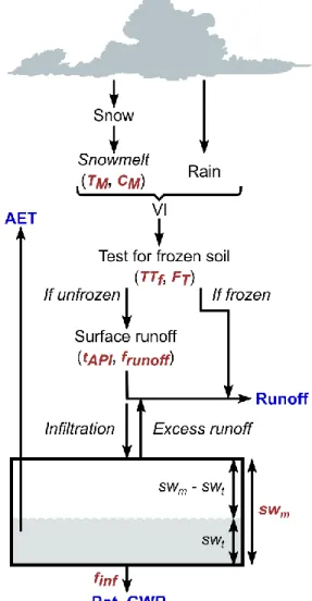
HydroBudget is a spatially distributed GWR model that computes a superficial water budget on grid cells of regional-scale watersheds. Runoff, actual evapotranspiration (AET), and potential GWR are simulated for each grid cell (Figure 1), with a monthly time step, and fluxes do not transfer from a cell to another (no water routing). The model inputs are distributed daily precipitation and temperature as well as distributed data of pedology, land cover, and slope. The model script is entirely coded in R and eight parameters need to be calibrated (Table 1).

Figure 1: HydroBudget processes including the eight calibrated parameters in red (from Dubois et al., submitted to HESS)

The model first determines whether precipitation occurs as rain or snow using a simple air temperature threshold (0°C – not a calibration parameter but can easily be modified in the code). If precipitation occurs as snow, it accumulates until air temperature rises above a threshold melting temperature (TM) at which snow is melted at a certain rate (CM) using the commonly used degree-day approach (Massmann, 2019). Snowmelt is added to rain to provide the available liquid water (vertical inflow - VI). As a simplified view of superficial conditions to freeze soil (Henry, 2007), the soil is considered frozen if air temperature has been below a given threshold (TTF) for a given number of days (FT). If the soil is frozen, the entire VI will directly produce runoff (R). If the soil is unfrozen, VI can runoff, infiltrate, be evapotranspired, and eventually percolate as potential GWR. Runoff is calculated using the runoff curve number (RCN) method (USDA-NRCS, 2004; 2007). The RCN method assesses soil ability to produce runoff or infiltration for each precipitation event, based on pedology, land cover, slope, and the antecedent moisture conditions. The soil runoff capacity gradually increases when antecedent moisture conditions change from “dry” (wilting point) to “normal” (default value in the model) to “wet” (field capacity) (Hawkins et al., 2019; Ponce and Hawkins, 1996). Relative runoff capacity variations from the default value are based on algorithms developed for the local context (for Quebec: Gagné et al., 2013; Monfet, 1979) or for a general context (Lal et al., 2019). The switch from one soil moisture stage to the next occurs when the antecedent precipitation index (API), corresponding to the sum of the VI of the previous days (5 by default in the original RCN method), reaches a threshold value for dry or wet conditions, often determined for the local context as well (Miliani et al., 2011; Monfet, 1979). Lal et al. (2015) suggested that the API varies between one and five days (the original value of the RCN method). Therefore, the time constant to compute the API (tAPI) is a calibration parameter in HB (i.e., does not vary during a given simulation). If tAPI increases (or decreases), then runoff increases (or decreases). In HB, the RCN method is used on a cell-by-cell basis, similar to what is done in the Soil Water Assessment Tool (SWAT; Arnold et al., 2012; Neitsch et al., 2002). A second parameter, the runoff factor (frunoff), is needed to modulate the VI partitioning between R and infiltration into the soil reservoir (Inf) (Equation 1), and should tend toward 1 (i.e., no influence of the factor on runoff – scenario case where the runoff was calibrated separately).

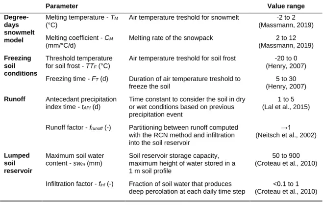
Table 1 : HydroBudget calibration parameters (adapted from Dubois et al., submitted to HESS)

Parameter Value range

Degree-days snowmelt model Melting temperature - TM (°C)

Air temperature treshold for snowmelt -2 to 2

(Massmann, 2019) Melting coefficient - CM

(mm/°C/d)

Melting rate of the snowpack 2 to 12

(Massmann, 2019)

Freezing soil conditions

Threshold temperature for soil frost - TTF (°C)

Air temperature treshold for soil frost -20 to 0

(Henry, 2007) Freezing time - FT (d) Duration of air temperature treshold to

freeze the soil

5 to 30 (Henry, 2007)

Runoff Antecedant precipitation index time - tAPI (d)

Time constant to consider the soil in dry or wet conditions based on previous precipitation event

1 to 5 (Lal et al., 2015)

Runoff factor - frunoff (-) Partitioning between runoff computed

with the RCN method and infiltration into the soil reservoir

→1

(Neitsch et al., 2002)

Lumped soil reservoir

Maximum soil water content - swm (mm)

Soil reservoir storage capacity, maximum height of water stored in a 1 m soil profile

50 to 900 (Croteau et al., 2010)

Infiltration factor - finf (-) Fraction of soil water that produces

deep percolation at each daily time step

<0.1 to 1 (Croteau et al., 2010)

The maximum soil water content (swm) corresponds to the maximum height of water stored in a 1 m soil profile (i.e., 1 m multiplied by total porosity; constant through time). If the available storage in the soil reservoir is sufficient (i.e., the difference between swm and soil water content from the previous time step swt-1 exceeds infiltration), the portion of VI that is not mobilized through runoff (Inf) infiltrates into the soil reservoir (Equation 2). If the available soil storage is insufficient to accommodate the incoming infiltration, excess is added to runoff (saturation excess – Excess R) (Equation 3, Equation 4). Finally, the part of VI that flow at the surface (runoff) per time step (Total R) corresponds to the sum of R and the Excess R (Equation 5) Potential evapotranspiration (PET) is calculated using the formula of Oudin et al. (2005), based on temperature and extraterrestrial radiation, estimated based on the latitude and the Julian Day. Actual evapotranspiration (AET) is calculated as the minimum between PET and the available water in the soil reservoir (Equation 6 to Equation 8). The residual soil water is mobilized as potential GWR using an infiltration factor (finf, constant through time), which controls the maximum infiltration capacity of the soil water. The infiltration factor is the fraction of soil water that produces deep percolation at each daily time step (Equation 10 to Equation 12). It is calculated as the ratio between the Darcy flux (under a unit gradient) and the parameter swm. For example, the conditions reported by Croteau et al. (2010), with till glacial deposits of 5.5 10-7 _{m/s hydraulic conductivity}

and a swm of 300 mm, result in a finf of 0.16. Higher values of finf are used for materials with higher hydraulic conductivity while finf of 1 corresponds to a reservoir that can be completely drained during one time step. Water that do not infiltrate is saved for the following day (Equation 11 and Equation 13). 𝑅 = 𝑓𝑟𝑢𝑛𝑜𝑓𝑓 × 𝑅𝑅𝐶𝑁 Equation 1 𝐼𝑛𝑓 = 𝑉𝐼 − 𝑅 Equation 2 If (swm – swt ) ≥ Inf Then 𝐸𝑥𝑐𝑒𝑠𝑠 𝑅 = 0 Equation 3 Else 𝐸𝑥𝑐𝑒𝑠𝑠 𝑅 = 𝐼𝑛𝑓 − (𝑠𝑤𝑚− 𝑠𝑤𝑡) Equation 4 𝑇𝑜𝑡𝑎𝑙 𝑅 = 𝑅 + 𝐸𝑥𝑐𝑒𝑠𝑠 𝑅 Equation 5 If swt + Inf > PET Then 𝐴𝐸𝑇 = 𝑃𝐸𝑇 Equation 6 𝑠𝑤𝑡′ = 𝑠𝑤𝑡+ 𝐼𝑛𝑓 − 𝐴𝐸𝑇 Equation 7 Else 𝐴𝐸𝑇 = 𝑠𝑤𝑡+ 𝐼𝑛𝑓 Equation 8 𝑠𝑤𝑡′ = 0 Equation 9 If swt’ > 0 Then 𝐺𝑊𝑅 = 𝑠𝑤𝑡′ × 𝑓𝑖𝑛𝑓 Equation 10 𝑠𝑤𝑡′′ = 𝑠𝑤𝑡′ − 𝐺𝑊𝑅 Equation 11 Else 𝐺𝑊𝑅 = 0 Equation 12 𝑠𝑤𝑡′′ = 0 Equation 13 R = runoff (mm)

frunoff = runoff factor (-)

RRCN = runoff computed with the RCN method (mm)

Inf = infiltration to the soil reservoir (mm) VI = vertical inflow (mm)

swm = maximum soil water content in the soil reservoir (mm)

swt = soil water content at the end of the previous time step (mm)

Excess R = excess runoff produced by the soil reservoir (mm) Total R = total runoff at the end of the time step (mm)

PET = potential evapotranspiration (mm) AET = actual evapotranspiration (mm)

swt’ = soil water content at the end of the current time step, after the AET computation (mm)

GWR = potential groundwater recharge (mm)

finf = infiltration factor (-)

Although daily time steps are used for the calculation, the simulated outputs are integrated on a monthly time step. The sum of runoff and potential GWR (Total R + GWR) on the entire watershed is considered to be equal to total river flow at the watershed outlet. Potential GWR (GWR) is considered to be equal to baseflow.

HydroBudget calculates potential GWR, i.e., the percolating water that can reach the saturated zone if 1) the geological material below the soil horizon allows deep percolation, 2) no additional storage or losses occur in the unsaturated zone below the soil, and 3) no significant evapotranspiration occurs from groundwater (Doble and Crosbie, 2017). Actual GWR corresponds to the part of potential GWR that will reach the water table, and potential GWR is therefore a maximum.

If the local RCN application conditions are strictly applied (Monfet, 1979), superficial water bodies and wetlands would have the maximum RCN value (100), therefore producing 100% of runoff from the precipitation and keeping the soil reservoir empty (preventing AET and potential GWR). To avoid that configuration, RCN values of grid cells of water and wetlands are artificially lowered to a value of 10 to allow the majority of VI to infiltrate into a reservoir, which percolation capacity is null (no potential GWR – coded in HB R script). With this setup, high evapotranspiration (AET ≈ PET) and high excess runoff are produced, compensating for the artificially lowered primary runoff. Although wetlands do not produce potential GWR in HB, it is well known they are often connected to regional groundwater systems (e.g., Bourgault et al., 2014). Therefore, wetland representation in HB is a regional simplification that might need to be improved in future versions.

2.2 Input data

2.2.1 Grid building for the study area

To simulate GWR with HB, the study area needs to be divided into a grid to compute the water budget for each grid cells. Although the simplest grid is a grid of regular square cells, a grid of various shaped cells could be used as well, thus requiring modifying the initial script of the model. The simplest way of building a grid on a study area is to compute the RCN (cf. section Erreur ! Source du renvoi introuvable.) and rasterize the spatially distributed RCN with the desired spatial resolution. In that case, the raster pixel resolution could be used as the spatial resolution of the model.

2.2.2 Climate data

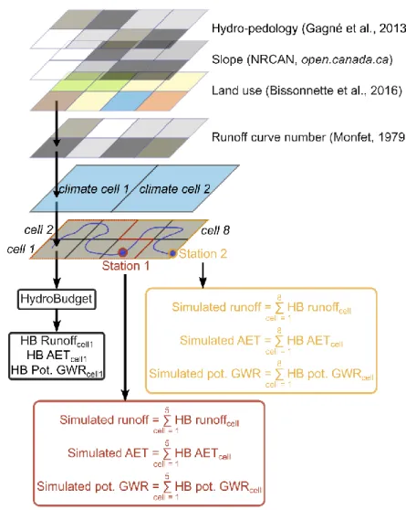
HydroBudget uses spatially distributed daily total precipitation (rainfall and snowfall) and mean daily temperature. In Quebec, this data is available from the interpolated climate grid by Bergeron (2016) for the period 1691-2017, with very limited error in southern Quebec (RMSE of 3 mm/d for precipitation, 2.5°C for minimal temperature, and 1.5°C for maximal temperature). Each cell in the climate grid must be associated with each cell (RCN cells) of the study area grid to run HydroBudget (Figure 2).

2.2.3 Runoff Curve Number

To compute the spatialized water budget, spatialized RCN are needed at the resolution of the grid defined for the study area (cf. section 2.2.1; Figure 2). The RCN method is fully described in USDA (2004; 2007) and its adaptation for the province of Quebec has been described by Monfet (1979). Land use, mean slope, and “hydro-pedology” classification are needed to compute the RCN over a cell, (Table 2). The hydro-pedology classification describes in a qualitative way the ability of the superficial layer of soil to generate runoff or infiltration, with four levels ranging from high infiltration capacity to low infiltration capacity. Gagné et al. (2013) developed the link between the pedologic maps of Quebec and the hydro-pedology classification.

Once the RCN attribution is done, RCN values in “normal humidity conditions” are obtained (RCN II). These values evolve depending on the moisture conditions, from wet (RCN I) to dry (RCN III), computed from RCN II values by Equation 14 and Equation 15 for southern Quebec (adapted from Monfet, 1979).

𝑅𝐶𝑁 𝐼 = 0.00865 × 𝑅𝐶𝑁 𝐼𝐼2_{+ 0.0145 × 𝑅𝐶𝑁 𝐼𝐼 + 7.39846 Equation 14}

Figure 2: Composition of input data for HydroBudget in southern Quebec

The threshold values of antecedent precipitation index (API), the sum of VI of the x previous day (determined with the parameter tAPI in HB), trigger the change from the RCN II conditions (“normal”) to RCN I or RCN III are defined in Quebec by Monfet (1979) for each season. An RCN value is therefore associated for each computational iteration (RCNit), depending on the season and the recent precipitation. For each iteration, runoff (RRCN) is computed as follows:

𝑅𝑅𝐶𝑁=

[𝑉𝐼 − 0.2 × (1 000 𝑅𝐶𝑁⁄ 𝑖𝑡− 10)] 2

𝑉𝐼 − 0.8 × (1 000 𝑅𝐶𝑁⁄ 𝑖𝑡− 10)

Equation 16

Although this version of the RCN method is implemented in the HB code, it could easily be modified for another locally developed version.

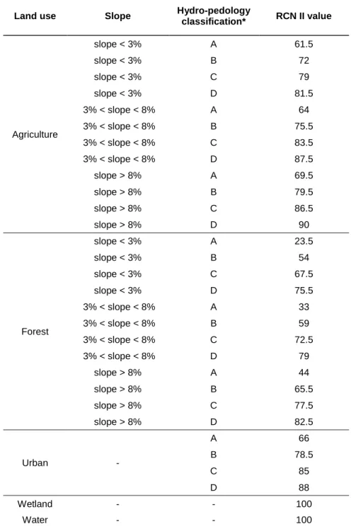
Table 2: Attribution of the RCN value for Quebec adapted from Monfet (1979)

Land use Slope Hydro-pedology

classification* RCN II value Agriculture slope < 3% A 61.5 slope < 3% B 72 slope < 3% C 79 slope < 3% D 81.5 3% < slope < 8% A 64 3% < slope < 8% B 75.5 3% < slope < 8% C 83.5 3% < slope < 8% D 87.5 slope > 8% A 69.5 slope > 8% B 79.5 slope > 8% C 86.5 slope > 8% D 90 Forest slope < 3% A 23.5 slope < 3% B 54 slope < 3% C 67.5 slope < 3% D 75.5 3% < slope < 8% A 33 3% < slope < 8% B 59 3% < slope < 8% C 72.5 3% < slope < 8% D 79 slope > 8% A 44 slope > 8% B 65.5 slope > 8% C 77.5 slope > 8% D 82.5 Urban - A 66 B 78.5 C 85 D 88 Wetland - - 100 Water - - 100

2.3 Calibration method

For a given watershed, the HydroBudget model is calibrated, based on the following hypotheses: 1) surface watersheds match hydrogeological watersheds, 2) the rivers drain unconfined aquifers, and 3) the watershed response time is shorter than one month, thus compensating for the absence of water routing. Under these conditions, for any given watershed, monthly potential GWR should be similar to monthly river baseflow at the outlet, and the sum of monthly runoff and monthly potential GWR should be equal to the total flow at the outlet (although monthly flows are considered, daily time steps are used in the calculations).

In the current version of HB, baseflows are estimated from the river flow time series following Ladson et al. (2013) proposition for a standard approach of the Lyne and Hollick filter (Lyne and Hollick, 1979), using a stochastic calibration and 30 passes of the filter. Total flows and baseflows are divided by the area of the given watershed to provide flow values in mm/yr and thus facilitate the comparison of calibration results between watersheds of very different sizes. The model is calibrated on a gauging station (or simultaneously calibrated on a group of gauging stations) using the automatic calibration procedure of the R package caRamel (Monteil et al., 2020).

A script was developed to optimize the eight HB parameters on a watershed, based on a single gauging station or simultaneously on all the gauging stations of the watershed, following the automatic calibration procedure of the R package caRamel (Monteil et al., 2020). Developers of the caRamel code recommend using up to 5 000 model calls per calibration, with several successive optimizations to confirm the reproducibility of the results. Model performance is assessed with the Kling–Gupta Efficiency (KGE, Gupta et al., 2009) calculated for monthly measured river flows and simulated river flow (KGEqtot), as well as monthly baseflow and monthly potential GWR (KGEqbase). In the script, each river flow time series is divided into a calibration period (first two thirds) and a validation period (last third), therefore allowing to compute the objective functions per period per gauging station. In the case of a group of gauging station,

KGEqtot corresponds to the mean of the individual KGEqtot per station and the KGEqbase to the mean of the individual KGEqbase per station.

The caRamel algorithm (Monteil et al., 2020), a combination of the multi-objective evolutionary annealing simplex algorithm (MEAS; Efstratiadis and Koutsoyiannis, 2008) and the non-dominated sorting genetic algorithm II (ε-NSGA-II; Reed and Devireddy, 2004), is used to calibrate the eight HB parameters to maximize KGEqtot and KGEqbase values. The algorithm produces an ensemble of parameter sets (called generation) to run the model and downscales the generation to the sets of parameters that optimize the objective functions and creates a new set of parameters

that produces better results. To produce new generations and ensure that the optimization tends toward a global maximum, the algorithm samples the parameter sets that individually maximize the two objective functions KGEqtot and KGEqbase, samples the parameter sets that maximizes the minimum values of the two objective functions and increases the variance of each parameter. Finally, the best compromise was chosen by identifying the highest value of mean KGE (KGEmean):

𝐾𝐺𝐸𝑚𝑒𝑎𝑛= 𝑥 × 𝐾𝐺𝐸𝑞𝑡𝑜𝑡+ 𝑦 × 𝐾𝐺𝐸𝑞𝑏𝑎𝑠𝑒 Equation 17

The weights x and y attributed to each objective function in KGEmean can be set to arbitrary values, depending on the study’s objectives. For example, for the model developed to simulate GWR over southern Quebec, the set (x = 0.4; y = 0.6) was chosen to maximize the quality of the reproduction of the baseflows, considered as the proxy for GWR (KGEqbase), without dropping the benefits of the multi-objective optimization (Dubois et al., submitted to HESS).

2.4 Similarities with other models

In water budget models, GWR is computed as the residual of the water budget (Scanlon et al., 2002), therefore they are all based on similar processes (Table 3). They use precipitation as input and sometimes estimate interception, snow accumulation and snowmelt. The RCN method (USDA-NRCS, 2004; 2007) is a widely-used empirical method to compute runoff. It is used in HELP (Schroeder et al. 1994), SWAT (Neitsch et al., 2002), SWB (Westenbroek et al., 2010) and in the water balance GIS tool (Portoghese et al., 2005). WetSpass (Batelaan and De Smedt, 2007) and WGHM (Döll et al., 2003) use similar empirical methods, based on runoff coefficients to compute runoff as a ratio of precipitation. In HB, a freezing soil condition is used to produce 100% of runoff from the available water if the soil is frozen. This approach is not included in the models listed in Table 3, but WGHM accounts for freezing soil in permafrost and glacier areas (Döll et al., 2003). In all the models, the remaining water (precipitation minus runoff) is routed to the soil where evapotranspiration is removed based on potential evapotranspiration formulas, or based on specific land cover for WetSpass and WGHM (using crop and vegetation coefficients). The soil modelling widely varies depending on model complexity and modeling objectives. For example, HELP considers a 2 m layered soil columns (unsaturated zone) generating subsurface runoff and infiltration for each soil layer, and the excess water reaching the base of the soil column is considered as GWR (Croteau et al., 2010). Similarly, the water balance GIS tool uses soil hydraulic conductivity to partition infiltration water into sub-surface runoff or potential GWR (Portoghese et al., 2005). The SWB model uses the Thornthwaite soil moisture retention equations to estimate if

Bradbury, 2007). WGHM considers GWR as a portion of superficial runoff using an infiltration factor (Döll and Fiedler, 2008) while WetSpass computes GWR as the residual water of the water budget.

While being very similar to other water budget models, HB uses a simplified soil representation and the most accessible data as input and computes potential GWR, similarly to SWB and the water balance GIS tool (Table 3). HELP, WetSpass and WGHM produce actual GWR although only WetSpass take into account the feedback of the water table depth on the GWR. The potential GWR calculated in HB is mostly sensitive to the runoff factor (frunoff) and the infiltration factor (finf) equivalent to that found for SWB and WetSpass to a certain extent. The simulation of GWR with HELP, SWB, and WetSpass seem sensitive to unsaturated zone parameters as well, as the unsaturated zone processes in these models are relatively detailed.

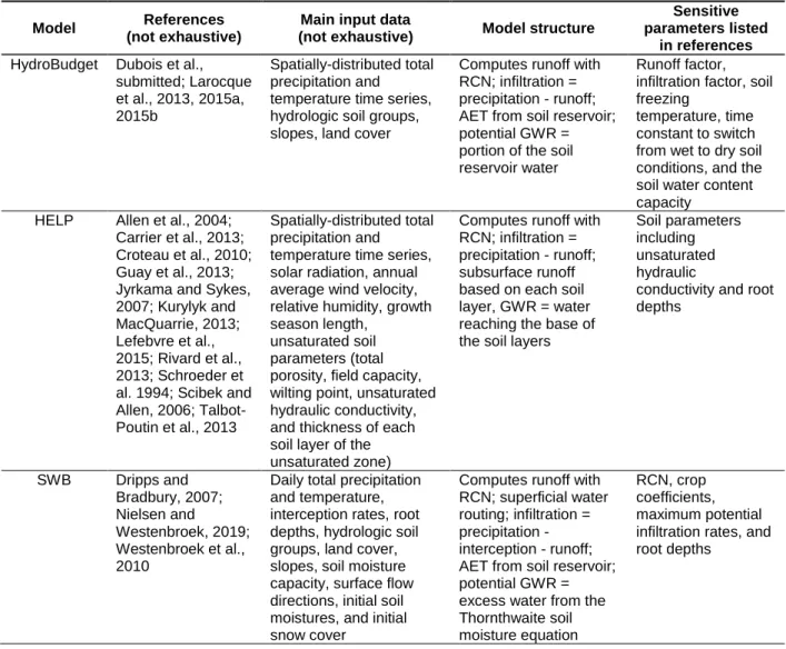
Table 3: Main characteristics of a selection of groundwater recharge water budget models

Model References (not exhaustive)

Main input data

(not exhaustive) Model structure

Sensitive parameters listed

in references

HydroBudget Dubois et al., submitted; Larocque et al., 2013, 2015a, 2015b

Spatially-distributed total precipitation and temperature time series, hydrologic soil groups, slopes, land cover

Computes runoff with RCN; infiltration = precipitation - runoff; AET from soil reservoir; potential GWR = portion of the soil reservoir water

Runoff factor, infiltration factor, soil freezing

temperature, time constant to switch from wet to dry soil conditions, and the soil water content capacity

HELP Allen et al., 2004;

Carrier et al., 2013; Croteau et al., 2010; Guay et al., 2013; Jyrkama and Sykes, 2007; Kurylyk and MacQuarrie, 2013; Lefebvre et al., 2015; Rivard et al., 2013; Schroeder et al. 1994; Scibek and Allen, 2006; Talbot-Poutin et al., 2013

Spatially-distributed total precipitation and temperature time series, solar radiation, annual average wind velocity, relative humidity, growth season length,

unsaturated soil parameters (total porosity, field capacity, wilting point, unsaturated hydraulic conductivity, and thickness of each soil layer of the unsaturated zone)

Computes runoff with RCN; infiltration = precipitation - runoff; subsurface runoff based on each soil layer, GWR = water reaching the base of the soil layers

Soil parameters including unsaturated hydraulic

conductivity and root depths SWB Dripps and Bradbury, 2007; Nielsen and Westenbroek, 2019; Westenbroek et al., 2010

Daily total precipitation and temperature, interception rates, root depths, hydrologic soil groups, land cover, slopes, soil moisture capacity, surface flow directions, initial soil moistures, and initial snow cover

Computes runoff with RCN; superficial water routing; infiltration = precipitation - interception - runoff; AET from soil reservoir; potential GWR = excess water from the Thornthwaite soil moisture equation

RCN, crop coefficients, maximum potential infiltration rates, and root depths

Model References (not exhaustive)

Main input data

(not exhaustive) Model structure

Sensitive parameters listed in references water balance GIS tool Portoghese et al., 2005 Spatially-distributed interannual monthly rainfall and PET, vegetation cover and monthly crop coefficients, soil-moisture contents, soil thickness and hydrologic soil groups, land cover (including the percentage of pervious/ impervious surfaces), slopes

Computes runoff with RCN; infiltration = precipitation - runoff; AET = PET corrected with crop coefficients and available soil moisture; computation of sub-surface runoff based on the soil texture, potential GWR = residual water of the water budget

n.a.

WetSpass Abdollahi et al.,

2017; Batelaan and De Smedt, 2007; Zomlot et al., 2015

Soil texture, groundwater depth, slope, rainfall, potential

evapotranspiration, number of rainy days, wind, temperature, and land cover with the detail of vegetated cover, bare soil, open water, and impervious surface on each grid cell

Computes runoff as a fraction of precipitation; Infiltration =

precipitation - interception - runoff; AET = PET corrected with crop coefficients; GWR = residual water of the water budget

Runoff coefficients, soil moisture coefficients, and interception parameters WGHM Döll and Fiedler, 2008; Döll et al., 2003 Spatially-distributed precipitation and temperature, number of wet days per month, cloudiness, daily

sunshine hours, land use, superficial drainage

Computes AET as the minimum of PET and the available soil water; runoff is a function of the difference

precipitation - AET and of the soil moisture; superficial water routing; GWR = percentage of runoff

3

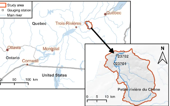
EXAMPLE FOR THE PETITE DU CHENE RIVER (QUEBEC)

An application example can be taken on the Petite du Chêne River watershed (460 km2_{), a St.}

Lawrence tributary located in southern Quebec (Figure 3). Two gauging stations monitored river flows mainly from 1993 to 2007 (gap of 6 days in 2005) for the station 23701 and from 2007 to 2017 for the station 23702. Interpolated climate data are available from 1961 to 2017 and distributed on 10x10 km grid (Bergeron, 2016). The application example will simulate the water budget on the watershed for the entire 1961-2017 period. The R scripts and input data can be requested to [email protected].

3.1 Folder 01-demonstration_HB.zip

The model scripts, the input data, the river flows time series, and the shape files (GIS) for the area are compressed in a .zip file “01-demonstration_HB.zip”:

 The folder 01-input contains the input data:

o alpha_lyne_hollick.csv: the statistically calibrated α following Ladson et al. (2013) procedure for the Lyne and Hollick (1979) baseflow computation for the two gauging stations (the baseflow computation itself is included in HB script) ;

o input_climate.csv: daily total precipitation (mm/d) and average daily temperature (°C) of the Quebec climate interpolated grid (Bergeron, 2016) from 1961/01/01 to 2017/12/31. The data are per climate cell, corresponding to the attribute “climate_cell” ;

o input_rcn.csv: the RCN values on a 500x500 m grid. A RCN value (attribute “RCNII”) for each grid cell of the watershed (attribute “cell_ID”) is given, with the corresponding climate cell (attribute “climate_cell”) and the coordinates of the center of each RCN cell in NAD83 Quebec Lambert (EPSG: 32198) ;

o input_rcn_gauging.csv: a table with the list of RCN cells that are located in each gauging station watershed. The table is composed of two attributes, the “cell_ID” that indicates the RCN cell, and the “gauging_stat” that indicates the associated gauging station. Since the watersheds of the two gauging stations are overlaying, RCN cells can be associated with each of them; in that case, the RCN cell ID will appear twice in the table, once with each gauging station ;

o observed_flow.csv: all the measured river flow (mm/d) of the 2 gauging stations, one table attribute for each station, for the entire time period covered by the climate data. Unavailable data (including if flow measurements do not exist for a given period) are marked with a “NA” (Not Available).

 The folder 02-GIS_petite_du_chene contains the shapefiles and rasters (GIS) in NAD83 Quebec Lambert (EPSG: 32198) with:

o Shapefiles (.shp) for the rivers (lines), the location of the gauging stations (points), the climate grid (polygons), the watersheds of the gauging stations (polygons), the grid for each gauging station with the cell ID and the associated climate cell (polygons), the grid for the entire watershed of the Petite du Chêne River with the cell ID and the associated climate cell (polygons), and the watershed of the Petite du Chêne River (polygon);

o R_landuse_NAD83.tif the raster of the reclassified land use from Bissonnette et al. (2016) containing:

Criteria Code pixel Number of pixels

Agriculture 1 703

Forest 2 869

Wetland 3 299

Water 4 10

Urban 5 32

Harvested forest (associated with forest) 6 60

Bare soil (associated with urban) 7 1

o R_pedohydro_NAD83.tif the raster of the hydro-pedologic criteria containing:

Criteria Code pixel Number of pixels

A – very well drained 1 398

B – well drained 2 486

C – poorly drained 3 932

D – very poorly drained 4 158

o R_RCN_NAD83.tif the raster of the RCN values per grid cell ranging from 23.5 to 100 o R_slope_NAD83.tif the raster of the slopes reclassified in 3 categories based on the DEM

from NRCAN (https://open.canada.ca/data/en/dataset) containing:

Criteria Code pixel Number of pixels

Slope < 3% 1 1971

3% < slope < 8% 2 3

Slope > 8% 3 0

 00-demonstration_HB: an R project that opens the two R scripts 01-HydroBudget.R and 02-HB_caRamel.R directly (if it does not, load manually the two scripts in the R project);

 01-HydroBudget.R: an R script that contains the HB code and references to the inputs data located in the folder 01-input previously detailed. This code can be used to run HB on the Petite du Chêne River with a single set of parameters. It will automatically simulate the water budget

on the watershed, create a folder with the results, save the results for the entire watershed (spatially distributed and averaged on the watershed) as well as averaged for each gauging station, compute the objective functions for the 2 gauging stations per period (KGEqtot and

KGEqbase for both calibration and validation periods), and save a summary of the simulation in

a separate csv file;

 02-HB_caRamel.R: a script that contains the automatic calibration procedure with the caRamel algorithm.

3.2 Run HydroBudget with the 01-HydroBudget.R script

This script contains an R function to run HB. Comments for each step that the user needs to complete are included. The script is divided in 4 sections:

 Section 1-Load the packages

All the packages need to be loaded before running the model. Please install them if it is the first use of the model. The package “doSNOW” is optional (just to add a loading bar during the different computational steps of the model) and the package “doMC” replaces the package “doParallel” if the model is used on a computer with an exploitation system different than Windows.

 Section 2-Load the input data for the simulation and enter the parameters values

This section is detailed in several subsections. The first step (2.1) consists of defining the path to the demonstration folder, from which the code will create a folder “YYYY_MM_DD_HH_mm_simulation_HydroBudget” to store all the results. Then the input data will be loaded (2.2), and the user will have to assign values to the model parameters (2.3). Parameter values from Dubois et al. (submitted) are pre-assigned. The simulation period and the spatial resolution are defined in 2.4 (values pre-assigned for the example), and the parallel computing options are given in 2.5. In the following code, the snow accumulation and snow melt per climate cell and the water budget partitioning per grid cell of the study are simulated simultaneously on several cells with parallel loops (foreach in R). The calculation time is therefore significantly decreased since R simultaneously computes the task for several cells.

 Section 3-HB function

This section creates an R function called “HB” in the local environment. No action is required by the user here except executing all the lines. The function will run HB in parallel on all the grid cells of the watershed following Figure 1 processes. The input data of the function are all defined in section 2. A first parallel loop will run the degree-day model and compute Oudin PET on each climate cell for the chosen simulation period and a second parallel loop will run HB water partitioning on each RCN cell. For the parallel loops, the options before starting the loop, to add the progression bars, and to finish the loops need to be changed if the model is run on a computer with a Windows environment or not (options for the progression bar and the non-Windows environment are muted by default).

In case the RCN method need to be adapted to another version of the method, changes need to be done in the subsections 3.8.1.3 to 3.8.1.5 of the parallel loop of the model.

 Section 4-Simulation with HB

This section run the HB function created during section 3. with the inputs defined in section 2. It will save the results in the folder created in subsection 2.1.:

o 01_bilan_spat_month.csv: the spatialized simulated water budget by RCN cell for all the RCN cells of the Petite du Chêne River with monthly time step

o 02_bilan_unspat_month.csv: the averaged simulated water budget on the Petite du Chêne River with monthly time step (not spatialized)

o 03_bilan_unspat_month_23701.csv and 03_bilan_unspat_month_23702.csv: the averaged water budget per gauging station (not spatialized) with the observed flow and baseflows (attributes “q” and “qbase”)

o 04-simulation_metadata.csv: the summary of the simulation, with the used parameters, the details of the calibration and validation periods for each gauging station, the objective functions KGEqtot and KGEqbase per gauging station for calibration and validation periods, an averaged water budget per gauging station, and the averaged objective functions for the entire watershed

o 05_interannual_runoff_NAD83.tif,06_interannual_aet_NAD83.tif,

07_interannual_gwr_NAD83.tif: rasters of the corresponding variable with interannual values over the simulation period in NAD83 Quebec Lambert (EPSG: 32198)

3.3 Run the automatic calibration with the 02-HB_caRamel.R script

This code structure is similar to the script 01-HydroBudget.R. Sections 1 and 2 are dedicated to the packages to load and the input data to select. Section 3. creates a function in the local R environment which goal is to compute KGEqtot and KGEqbase (mean of the individual values for each gauging station) and return their values during the calibration period. However, the function still saves a short summary of the run in a file “simulation_metadata.csv”. The parameters for the optimization with caRamel are in section 4 and more detailed are available on the caRamel package page (https://cran.r-project.org/web/packages/caRamel/index.html) and publication (Monteil et al., 2020). The caRamel function iterates runs of the model with new sets of parameters and computes the objective functions for each run calling the HB function defined in section 3. Range of variation for each parameter can be found in Dubois et al. (submitted) (Table 1). Results of the optimization are saved in the subsection 4.2, and a loop is used to bind all the simulation summary files into a single file. The extraction of the best compromises from the optimization is detailed in section 5, where weights of each objective function can be set up and the number of best compromises to extract chosen.

REFERENCES

Abdollahi, K., Bashir, I., Verbeiren, B., Harouna, M. R., Van Griensven, A., Huysmans, M. and Batelaan, O. (2017). A distributed monthly water balance model: formulation and application

on Black Volta Basin. Environmental Earth Sciences, 76:198(5), 18. doi:

10.1007/s12665-017-6512-1

Allen, D. M., Mackie, D. C. et Wei, M. (2004). Groundwater and climate change: a sensitivity

analysis for the Grand Forks aquifer, southern British Columbia, Canada. Hydrogeology

Journal, 12(3), 270-290. doi: 10.1007/s10040-003-0261-9

Arnold, J. G., Kiniry, J. R., Srinivasan, R., Williams, J. R., Haney, E. B. and Neitsch, S. L. (2012).

Soil Water Assessment Tool - Input/Ouput documentation - Version 2012 (TR-439). Texas

Water Resources Institute.

Batelaan, O. and De Smedt, F. (2007). GIS-based recharge estimation by coupling surface–

subsurface water balances. Journal of Hydrology, 337(3), 337-355. doi: 10.1016/j.jhydrol.2007.02.001

Bergeron, O. (2016). Guide d’utilisation 2016 - Grilles climatiques quotidiennes du Programme de

surveillance du climat du Québec, version 2 (User guide 2016 – Daily climate grids from the Quebec Climate monitoring program, version 2). Québec City (Canada) : ministère du

Développement durable, de l’Environnement et de la Lutte contre les changements climatiques, Direction du suivi de l’état de l’environnement.

Bissonnette, J., Demers, A. and Lavoie, S. (2016). Utilisation du territoire. Méthodologie et

description de la couche d’information géographique (Land use. Methodology and overview of the GIS layer) (Version 1.4). Québec City (Canada) : Gouvernement du Québec, Ministère du

Développement durable, de l’Environnement et de la Lutte contre les changements climatiques.

Bourgault, M. A., Larocque, M. and Roy, M. (2014). Simulation of aquifer-peatland-river

interactions under climate change. Hydrology Research, 45(3), 425-440. doi: 10.2166/nh.2013.228

Carrier, M.-A., Lefebvre, R., Rivard, C., Parent, M., Ballard, J.-M., Benoit, N., … Lavoie, D. (2013).

Portrait des ressources en eau souterraine en Montérégie Est, Québec, Canada (Overview of groundwater resources of eastern Monteregie, Quebec, Canada, Quebec Groundwater Knowledge Acquisition Program report) [Rapport PACES](R-1433). Québec City (Canada) :

INRS, CGC, OBV Yamaska, IRDA, Ministère du Développement durable, de l’Environnement, de la Faune et des Parcs. https://rqes.ca/paces-monteregie-est/

Croteau, A., Nastev, M. and Lefebvre, R. (2010). Groundwater Recharge Assessment in the

Chateauguay River Watershed. Canadian Water Resources Journal, 35(4), 451-468, world.

doi: 10.4296/cwrj3504451

Doble, R. C. and Crosbie, R. S. (2017). Review: Current and emerging methods for

catchment-scale modelling of recharge and evapotranspiration from shallow groundwater. Hydrogeology

Journal, 25(1), 3-23. doi: 10.1007/s10040-016-1470-3

Döll, P. and Fiedler, K. (2008). Global-scale modeling of groundwater recharge. Hydrology and Earth System Sciences, 12(3), 863-885. doi: https://doi.org/10.5194/hess-12-863-2008

Döll, P., Kaspar, F. and Lehner, B. (2003). A global hydrological model for deriving water

availability indicators: model tuning and validation. Journal of Hydrology, 270(1), 105-134. doi:

10.1016/S0022-1694(02)00283-4

Dripps, W. R. and Bradbury, K. R. (2007). A simple daily soil–water balance model for estimating

the spatial and temporal distribution of groundwater recharge in temperate humid areas.

Hydrogeology Journal, 15(3), 433-444. doi: 10.1007/s10040-007-0160-6

Dubois, E., Larocque, M., Gagné, S. and Meyzonnat, G. (2021 – Submitted to HESS). Simulation

of long-term spatiotemporal variations in regional-scale groundwater recharge: Contributions of a water budget approach in southern Quebec. Hydrology and Earth Science System.

Efstratiadis, A. and Koutsoyiannis, D. (2008). Fitting Hydrological Models on Multiple Responses

Using the Multiobjective Evolutionary Annealing-Simplex Approach. In R. J. Abrahart, L. M. See

and D. P. Solomatine (dir.), Practical Hydroinformatics: Computational Intelligence and Technological Developments in Water Applications (p. 259-273). Berlin, Heidelberg : Springer. doi: 10.1007/978-3-540-79881-1_19

Gagné, G., Beaudin, I., Leblanc, M., Drouin, A., Veilleux, G., Sylvain, J.-D. and Michaud, A. (2013).

Classement des séries de sols minéraux du Québec selon les groupes hydrologiques (Classification of Quebec mineral soil types by hydrologic groups, final report) [Rapport final].

Québec City (Canada) : IRDA.

https://www.irda.qc.ca/assets/documents/Publications/documents/gagne-et-al-2013_rapport_classement_sols_mineraux_groupes_hydro.pdf

Guay, C., Nastev, M., Paniconi, C. and Sulis, M. (2013). Comparison of two modeling approaches

for groundwater–surface water interactions. Hydrological Processes, 27(16), 2258-2270. doi:

10.1002/hyp.9323

Gupta, H. V., Kling, H., Yilmaz, K. K. and Martinez, G. F. (2009). Decomposition of the mean

squared error and NSE performance criteria: Implications for improving hydrological modelling.

Journal of Hydrology, 377(1), 80-91. doi: 10.1016/j.jhydrol.2009.08.003

Hawkins, R. H., Theurer, F. D. and Rezaeianzadeh, M. (2019). Understanding the Basis of the

Curve Number Method for Watershed Models and TMDLs. Journal of Hydrologic Engineering,

24(7), 06019003. doi: 10.1061/(ASCE)HE.1943-5584.0001755

Henry, H. A. L. (2007). Soil freeze–thaw cycle experiments: Trends, methodological weaknesses

and suggested improvements. Soil Biology and Biochemistry, 39(5), 977-986. doi:

10.1016/j.soilbio.2006.11.017

Jyrkama, M. I. and Sykes, J. F. (2007). The impact of climate change on spatially varying

groundwater recharge in the grand river watershed (Ontario). Journal of Hydrology, 338(3),

237-250. doi: 10.1016/j.jhydrol.2007.02.036

Kurylyk, B. L. and Macquarrie, K. T. B. (2013). The uncertainty associated with estimating future

groundwater recharge: A summary of recent research and an example from a small unconfined aquifer in a northern humid-continental climate. Journal of hydrology, 492, 244-253. doi:

10.1016/j.jhydrol.2013.03.043

Ladson, A. R., Brown, R., Neal, B. and Nathan, R. (2013). A Standard Approach to Baseflow

Separation Using The Lyne and Hollick Filter. Australasian Journal of Water Resources, 17(1),

25-34. doi: 10.7158/13241583.2013.11465417

Lal, M., Mishra, S. K. and Kumar, M. (2019). Reverification of antecedent moisture condition

dependent runoff curve number formulae using experimental data of Indian watersheds.

CATENA, 173, 48-58. doi: 10.1016/j.catena.2018.09.002

Lal, M., Mishra, S. K. and Pandey, A. (2015). Physical verification of the effect of land features

and antecedent moisture on runoff curve number. CATENA, 133, 318-327. doi:

10.1016/j.catena.2015.06.001

Larocque, M., Gagné, S., Barnetche, D., Meyzonnat, G., Graveline, M.-H. and Ouellet, M.-A. (2015a). Projet de connaissance des eaux souterraines du bassin versant de la zone Nicolet

acquisition program of the Nicolet area and the lower Saint-François area, final report) [Rapport PACES]. Quebec City (Canada) : Université du Québec à Montréal - Département des

sciences de la Terre et de l’atmosphère, Ministère du Développement durable, de l’Environnement, de la Faune et des Parcs. http://rqes.ca/rqes/wp-

content/uploads/sites/72/2016/08/UQAM_-_PACES_NSF_-_Rapport_synth%C3%A8se_Final_tailler%C3%A9duite-1.pdf

Larocque, M., Meyzonnat, G., Ouellet, M.-A., Graveline, M.-H., Gagne, S., Barnetche, D. and Dorner, S. (2015b). Projet de connaissance des eaux souterraines de la zone de

Soulanges - Rapport final (Quebec groundwater knowledge acquisition program of Vaudreuil-Soulanges area, final report) [Rapport PACES]. Quebec City (Canada) : Université du Québec

à Montréal - Département des sciences de la Terre et de l’atmosphère, Ministère du Développement durable, de l’Environnement et de la Lutte contre les Changements Climatiques. https://rqes.ca/paces-vaudreuil-soulanges/

Larocque, M., Gagné, S., Tremblay, L. and Meyzonnat, G. (2013). Projet de connaissances des

eaux souterraines du bassin versant de la rivière Bécancour et de la MRC de Bécancour - Rapport final (Quebec groundwater knowledge acquisition program of the Bécancour River watershed and the Bécancour municipality, final report) [Rapport PACES]. Quebec City

(Canada) : Université du Québec à Montréal - Département des sciences de la Terre et de l’atmosphère, Ministère du Développement durable, de l’Environnement, de la Faune et des Parcs. https://rqes.ca/paces-becancour/

Lefebvre, R., Ballard, J.-M., Carrier, M.-A., Vigneault, H., Beaudry, C., Bertholt, L., … Molson, J. (2015). Portrait des ressources en eau souterraine en Chaudière-Appalaches, Québec,

Canada - Rapport final (version révisée) (Overview of Chaudière – Appalachians groundwater resources, Quebec groundwater knowledge acquisition program, final report, corrected version) [Rapport PACES](INRS R-1580). Quebec City (Canada) : Institut National de la

Recherche Scientifique (INRS), Institut de Recherche et Développement en Agroenvironnement (IRDA), Regroupement des organismes de bassins versants de la Chaudière-Appalaches, Ministère du Développement durable, de l’Environnement et de la Lutte contre les Changements Climatiques. https://rqes.ca/paces-chaudiere-appalaches/ Lyne, V. and Hollick, M. (1979). Stochastic time-variable rainfall-runoff modelling (vol. 1979, p.

89-93). Presented in Proceedings of the Hydrology and Water Resources Symposium, Perth : Institute of Engineers Australia National Conference.

Massmann, C. (2019). Modelling Snowmelt in Ungauged Catchments. Water, 11(2), 301. doi: 10.3390/w11020301

Miliani, F., Ravazzani, G. and Mancini, M. (2011). Adaptation of Precipitation Index for the

Estimation of Antecedent Moisture Condition in Large Mountainous Basins. Journal of

Hydrologic Engineering, 16(3), 218-227. doi: 10.1061/(ASCE)HE.1943-5584.0000307

Monfet, J. (1979). Evaluation du coefficient de ruissellement à l’aide de la méthode SCS modifiée

(Evaluation of the runoff coefficient computation with the modified SCS method). Québec City

(Canada) : Bibliothèque nationale du Québec.

Monteil, C., Zaoui, F., Moine, N. L. and Hendrickx, F. (2020). Multi-objective calibration by

combination of stochastic and gradient-like parameter generation rules – the caRamel algorithm. Hydrology and Earth System Sciences, 24(6), 3189-3209. doi: https://doi.org/10.5194/hess-24-3189-2020

Neitsch, S. L., Arnold, J. G., Kiniry, J. R., Williams, J. R. and King, K. W. (2002). Soil Water

Assessment Tool - Theoretical documentation - Version 2000 (TR-191). College Station,

Texas : Texas Water Resources Institute.

Nielsen, M. G. and Westenbroek, S. M. (2019). Groundwater recharge estimates for Maine using

a Soil-Water-Balance model—25-year average, range, and uncertainty, 1991 to 2015 [USGS Numbered Series](2019-5125). Reston, VA : U.S. Geological Survey. pubs.er.usgs.gov :

http://pubs.er.usgs.gov/publication/sir20195125

Oudin, L., Hervieu, F., Michel, C., Perrin, C., Andréassian, V., Anctil, F. and Loumagne, C. (2005).

Which potential evapotranspiration input for a lumped rainfall–runoff model? Part 2—Towards a simple and efficient potential evapotranspiration model for rainfall–runoff modelling. Journal

of Hydrology, 303(1), 290-306. doi: 10.1016/j.jhydrol.2004.08.026

Ponce, V. M. and Hawkins, R. H. (1996). Runoff Curve Number: Has It Reached Maturity? Journal of Hydrologic Engineering, 1(1), 11-19. doi: 10.1061/(ASCE)1084-0699(1996)1:1(11)

Portoghese, I., Uricchio, V. and Vurro, M. (2005). A GIS tool for hydrogeological water balance

evaluation on a regional scale in semi-arid environments. Computers & Geosciences, 31(1),

15-27. doi: 10.1016/j.cageo.2004.09.001

Reed, P. and Devireddy, V. (2004). Groundwater monitoring design: a case study combining

Multi-Objective Evolutionary Algorithms (vol. Volume 1, p. 79-100). WORLD SCIENTIFIC. doi: 10.1142/9789812567796_0004

Rivard, C., Lefebvre, R. and Paradis, D. (2013). Regional recharge estimation using multiple

methods: An application in the Annapolis Valley, Nova Scotia (Canada). Environmental earth

sciences, 71, 1389-1408. doi: 10.1007/s12665-013-2545-2

Scanlon, B. R., Healy, R. W. and Cook, P. G. (2002). Choosing appropriate techniques for

quantifying groundwater recharge. Hydrogeology Journal, 10(1), 18-39. doi:

10.1007/s10040-001-0176-2

Schroeder, P. R., Aziz, N. M., Lloyd, C. M. and Zappi, P. A. (1994). The Hydrologic Evaluation of

Landfill Performance (HELP) model: User’s guide for version 3 (EPA/600/R-94/168a).

Washington, DC : U.S. Environnemental Protection Agency Office of Research and Development.

Scibek, J. and Allen, D. M. (2006). Modeled impacts of predicted climate change on recharge and

groundwater levels. Water Resources Research, 42(11). doi: 10.1029/2005WR004742

Talbot Poulin, M.-C., Comeau, G., Tremblay, Y., Therrien, R., Nadeau, M.-M., Lemieux, J.-M., … Bérubé, S. (2013). Projet d’acquisition de connaissances sur les eaux souterraines du territoire

de la Communauté métropolitaine de Québec (PACES-CMQ) - Rapport final (Quebec groundwater knowledge acquisition program for the Quebec City metropolitan community, final report) [Rapport PACES]. Quebec City (Canada) : Université Laval - Département de géologie

et de génie géologique, Ministère du Développement durable, de l’Environnement et de la Lutte contre les changements climatiques. https://rqes.ca/paces-communaute-metropolitaine-de-quebec/

USDA-NRCS. (2004). Chapter 9 Hydrologic Soil-Cover Complexes. United State Department of

Agriculture-Natural Ressources Conservation Service.

https://www.nrcs.usda.gov/Internet/FSE_DOCUMENTS/stelprdb1043088.pdf

USDA-NRCS. (2007). Chapter 7 Hydrologic Soil Groups (2009e éd.). United State Department of

Agriculture-Natural Ressources Conservation Service.

https://directives.sc.egov.usda.gov/OpenNonWebContent.aspx?content=22526.wba

Westenbroek, S. M., Kelson, V. A., Dripps, W. R., Hunt, R. J. and Bradbury, K. R. (2010). SWB—

Zomlot, Z., Verbeiren, B., Huysmans, M. and Batelaan, O. (2015). Spatial distribution of

groundwater recharge and base flow: Assessment of controlling factors. Journal of Hydrology: