lamsade
LAMSADE
Laboratoire d’Analyse et Modélisation de Systèmes pour
l’Aide à la Décision
UMR 7243o
octobre 2016
Methodological problems in defining costs
used in industrial management decision models
Vincent Giard
CAHIER DU
376
Methodological problems in defining costs used in industrial
management decision models
Vincent Giard
*,***Emeritus Professor, Paris-Dauphine, PSL Research University, CNRS, 75016, Paris, France
**Affiliate Professor, EMINES School of Industrial Management, Université Mohammed VI Polytechnique, 43140 Ben Guerir, Maroc
Abstract: Articles dealing with industrial management decision-making generally
rely on a cost system to establish a global indicator and identify the best solution. Cost accounting is based on a number of assumptions as to production system operation that may be quite remote from those used in decision modelling. Our paper points out the origin of this inconsistency and that it may lead to irrelevant decisions.
Keywords: model costing, cost management, supply chain management
1. Introduction
An analysis of the impact of operational, tactical and strategic decisions always relies on a physical model of a production system of products (generic term that we use in this paper to refer to both goods and services), whose operation is affected by the decisions to be taken. Such decisions are described by quantitative variables (e.g. quantity to be ordered…) or qualitative variables (transportation routes, alternative investments …) that certain models translate into binary variables. These are called ‘order variables’ and they impact production system operation through a series of more or less complex causal relations that lie at the heart of the chosen model. These interactions determine the value of certain physical parameters (level of inventory, travelled mileage …) chosen for their impact on production system performance. In the more straightforward models that involve a small number of physical parameters, these parameters are often called ‘state variables’; we use this term in our paper, regardless of model complexity.
The effectiveness criteria (such as minimum service level required…) used in the models are often more stringent in non-profit production systems and they narrow the scope of possible decisions. In order to choose the most efficient
solution, one must refer to an economic criterion because no single solution ever consumes fewer of each production system resource, therefore standing out as the best solution. In certain simple problems, the criterion is physical and the economic objective is implicit: for example, where cost is a linear function of time or distance, one may reason indifferently in terms of a physical indicator or associated cost. Generally, however, economic evaluation relies on a valorization system that stems from cost accounting to calculate a global value indicator being the weighted sum of state variables (and, in certain decision-making issues, of binary order variables). Such weighting approach is a cost system implicitly based on a model of the production system’s operations. Such modelling may be quite remote from that used to analyze the physical consequences of the decisions to be taken. This discrepancy may ultimately disqualify the chosen solution as irrelevant.
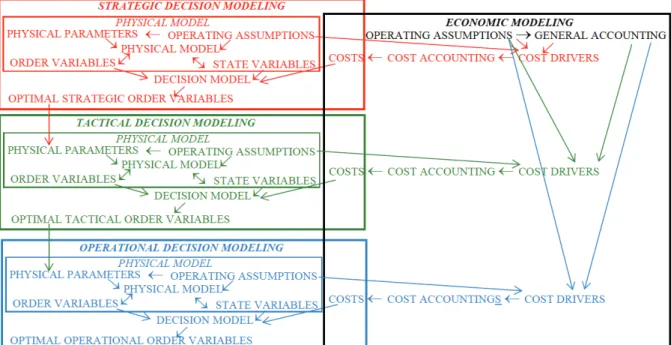
Let us turn to the foundations of these two types of model to describe physical production systems so as to be able to pinpoint potential sources of inconsistency. In order to avoid any risk of semantic confusion, we shall establish the distinction between the two types of model by calling them decision models and economic models respectively (the latter model underlying cost accounting). Figure 1 shows the relationship between these two approaches.
Fig. 1. Relationships between decision modelling and economic modelling.
2.
Physical representation characteristics of decision modelling
vs economic modelling
2.1 Underlying process models used in Decision Modelling
Decision modelling is chiefly characterized by a mix of three features: the degree of certainty of information used, the degree of reality of the system under review and its spatio-temporal granularity.
- Either the features of the production system and of its environment are considered to be known with certainty and the decisional issue is posed within a deterministic context, or they are not. Most of the time, where they are not,
these features are deemed to be known as random variables. Such characterization has an impact on the choice of technical model. In a random context and in straightforward fictional systems, analytical models use expectation; where they are complex, they rely on the Monte Carlo approach and involve recourse to spreadsheets or process simulation softwares. In a deterministic context, mathematical programming is quite relevant to the formalization of problems featuring simple causal relations, but a spreadsheet approach may be necessary where causal relations are complex.
- Production systems are either actual or fictional. The literature on operational research prefers relatively simple fictional systems to work out the analytical relation that describes the optimal solution for a type of decision-making issue (e.g. procurement management). But fictional systems can also be complex and use parametric cardinalities to produce a generic model for the problem (for example determination of a delivery route) via mathematical programming or graph theory. In certain cases they take the form of an algorithm of specific resolution. A number of research papers, prepared within the framework of industrial contracts, look into decision-making issues in connection with actual production systems. In this case, the model may lead to i) the assessment of decision-making scenarios (what-if analysis), ii) the formulation of an optimization problem where the level of complexity is low,
iii) the formulation of a simulation model or iv) a decision support system
(DSS) combining a scenario rationale with local optimizations and/or simulation. The proposed approach is often sufficiently generic to be transposable to similar production systems in similar decision-making issues. - The granularity used in the model, in its spatial and temporal dimensions, is a key element of decision model characterization. Time has multiple dimensions: mono or multi-period model, length of the period and horizon used in multi-period models. The granularity also involves spatial characterization, with varying levels of detail (or of aggregation) of resources and products. In general, the granularity is fine in operational decision analysis and more aggregated in other cases, except that many strategic decisions imply reference to a detailed model in order to ensure the robustness of a solution derived from an aggregated model.
2.2 Implicit, underlying, process modelling in Economic Modelling
General accounting involves matching physical and financial flows observed in a business so as to be able to perform periodic assessments of the results of its activity and the value of its assets. Such evaluation must comply with a number of rules as to the booking of certain expenses impacting corporate asset value
(Balance Sheet) for the reference period (accounting year). This information is intended for third parties (tax authorities, customers, suppliers, shareholders…) as well as for internal purposes (free cash flow, debt, receivables). This accounting treatment complies with a set of rules to defer investment expenses (depreciation expenses) and allocate to a period the financial flows from products purchased or sold during another period. Expenses are classified by nature e.g. raw materials, and by function e.g. sales, overheads…).
Cost accounting in the widest sense (several approaches are possible) processes the data generated by General Accounting to measure an entity’s (department, plant…) operating expenses, to measure the cost for an in-house service (e.g. dispatch of a container) or to measure the cost of a product. The computation of these costs poses two major methodological issues. While we focus on product cost in this paper we note that the same issues arise for both other types of cost.
- The first methodological issue is that of indirect cost allocation. These relate to services or inputs shared by several products (workshop energy expenses where there is only one meter, overheads…) and they may be shared (or not) between products.
- The second methodological issue is the impact of used capacity on the calculation of both direct and indirect costs (depreciation expenses of a machine dedicated to a type of production). A possible starting point is the actual level of activity − this making it difficult to compare in time and space − or reference to a “standard” level of activity. The latter solution, which is generally preferred, facilitates comparison in time (and space) but raises two issues: there can be no objective definition of a “standard” use of capacity and this could be a source of dispute, or even fraud. The gap between actual use of capacity and that deemed to be standard inevitably poses the problem of consistency between General Accounting and Cost Accounting, as the sum of costs in the latter could be quite different from that booked in accounting expenses.
Several solutions are available to address these issues and enable the calculation of partial costs and full costs. This does not lie within the scope of this paper whose aim is to show i) that the costs used in a valorization system stem from a production system workflow model that applies cost allocation rules over different periods of time, and ii) that used capacity (level of activity) assumptions and indirect cost allocation assumptions rely on causal relations that are debatable.
These costs are mainly computed for management control and should not be used indiscriminately for industrial management decision-making purposes. In this regard, some additional considerations are relevant to compute costs for decision-making purposes. The guideline is that the valorization system must provide that the benefits of the proposed decision versus a reference decision (that may be to do nothing) should be reflected in the organization’s financial results. To this end, the considerations set forth below should enter into the definition of the cost system used to assess industrial management decisions.
- The distinction between product direct and indirect cost, referred to above, depends on the level of aggregation used: an expense at a particular site may be indirect at the product level and direct at the product range level. Moreover, one is often led to consider entire product ranges as they all consume the same resources. The calculation of direct costs for a fictional product representing an entire family has to be the average weighted cost of the direct costs of the items comprising the family, where the weighting coefficients correspond to an average structure which cannot be deemed to be stable over time.
- Over the last two decades, activity based costing (ABC) stood out as a basic approach in cost accounting because it serves to reduce the arbitrary treatment of indirect costs. Its aim is to replace the direct causal relation “products consume resources” by the indirect causal relation “products consume activities that consume resources”. This approach encompasses the other cost accounting approaches as these may be deducted from it, which is why we adopt it in this paper. The concept of activity is wide; it can include production of an item as well as the launching of a production order for a set of products on a machine. This approach centered on cost drivers produces more relevant definitions of costs for decision modelling purposes.
- Economists have rapidly introduced the distinction between fixed and variable costs, fixed costs being independent from production volume. This concept, that can be extended to cost drivers, is crucial to decisional analysis, provided one explicitly defines the time horizon used for the decision-making exercise: where one looks at a few days’ horizon, previously hired utility workers are allocated to fixed costs (direct in the case of a production worker on a machine dedicated to a given product and indirect in the case of a maintenance worker) but, if the hiring decision has yet to be taken (for example to cope with a hike in activity over the relevant horizon), then this cost becomes variable and must be related to the production increase it would enable.
- Cost accounting focuses on the determination of product costs (in the widest sense, as already noted). A decision-making issue is formulated more in terms of costs stemming from a decision versus a reference decision (defined by the
values used for the order variables), which is not always clearly set forth. The optimal analytical solution of a fictional system (procurement rules, for example) are not pitched against a reference solution; use of such a reference for an actual case in order to optimize a recurring decision involves using a cost system whose value is not just to be able to calculate the order variables but also to measure the gain achieved when applying the optimal solution versus the status quo. This therefore should be reflected in the income statement, failing which the optimization is pointless. In the context of real-life systems, a decisional alternative (covering a set of order variables) will be assessed in relation to a benchmark decision/solution that may actually consist in taking no action (plant extension, for example) or to continue with what one already has, (replacement of a machine, for example). Such comparative economic analysis is called Incremental Cash Flow Report (ICFR) and serves to eliminate all expenses that are constant regardless of the alternative decision under review. Some decisions impact income. We shall leave these aside since they are obviously included in an ICFR.
- Let us add that the alternative decisions under review may impact several accounting periods, which calls for use of discounting to summarize the changes in cash flows calculated in the IFCR in order to compute Net Present Values.
3.
Examples of consequences of the above methodological
considerations
A number of costs drawn from cost accounting are useful for decision-modelling purposes provided the representation of the production system workflow is similar to that of the economic model used to determine these costs. Otherwise one faces an inconsistency which is generally overlooked in the literature. Since it is impossible to perform a thorough review of the implications of the above methodological considerations, we have decided to illustrate our discussion through a few typical cases. We shall first look at issues in connection with use of analytical solutions or of generic formulations that relate to operational or tactical decisions. We will then turn to methodological issues that arise in connection with decision models for strategic decision-making.
3.1 Issues raised by use of analytical solutions and by generic formulations of decision-making problems
These issues arise somewhat differently depending on whether one seeks to make concrete use of analytical relations from decision-making models based on fictional systems, or one seeks to design a generic model.
3.1.1 Use of analytical solutions
We will illustrate our discussion with procurement management where ordering costs, holding cost and stock out costs are typically considered. The former two costs pose similar methodological issues. The latter one raises specific issues. The models referred to here are described in several fairly exhaustive handbooks (for example, Giard, 2003; Silver et al., 1998).
Unit ordering cost and unit holding costs
In the deterministic version of the basic model (Wilson’s model), the order variables are the ordered quantity and the reorder point and the state variables are the average yearly number of orders and average number of products in stock. In the stochastic version, the averages are replaced by expectation and an additional state variable for “expected stock out” has to be added. The optimal analytical solution involves the unit costs associated to the state variable that corresponds to cost drivers. For ICFR purposes, the reference solution is the current solution regardless of whether the product exists or not. The application of these analytical relations to the resolution of concrete issues means that one has to specify correctly the contents of the unit costs in order to make sure the theoretical gains of switching from the current to the optimized solution show up in the income statement.
Take the example of a centralized order management desk. The new orders are a cost driver. The cost comprises a direct variable cost c (stationary, postal expenses…) and a share of the yearly cost K of running this desk which is an indirect cost. Where the desk handles n orders per year (to simplify, let’s assume that this is the standard level of activity), the standard cost of handling an order is K/n, which yields a unit ordering cost of c+K/n and a partial annual ordering cost of (c+K/ )n n n= ⋅c+K. Where the optimal procurement policy enables a 20 % reduction in the number of orders, the new annual partial cost of orders is equal to 0.8 (c+K/ )⋅n n provided that one is able to rapidly reallocate 20 % of resources to the origin of indirect cost K. Where this is not the case, the cost cut shrinks to
0.2 c⋅ ⋅n and the unit ordering cost of this new solution is a mere c+K/( 0.8)n⋅ , a sub-optimal value that calls for choice of a different solution. Where instead of a
reduction in the yearly number of orders, the switch to the optimal solution leads to an increase in this number, then the issue is that of order management desk under-staffing and need to cope with the workload increase.
The average number of inventory units is a cost driver that takes two forms, generating two unit cost components.
- For a business, an increase in the value of inventory either translates into an increase in working capital requirement or, where bank funding is not available for these assets, into a loss of short-term investment opportunities. This cost driver generates a variable direct cost corresponding to an
opportunity cost proportionate to the value of the product inventory and to the
interest rate.
- Inventory also involves yearly cost K′ (rental of warehouse, insurance, warden, energy, etc.) corresponding to an indirect cost that again, may be standardized on a volume basis. The definition of volume capacity Θ for the warehouse is tricky as it depends on the standard level of activity and on the degree of offsetting at all times between the high and low levels of inventory for each warehoused items. Where the current solution leads to keep volume θ in the warehouse for the considered product, the holding cost must include an additional storage cost K θ/′⋅ Θ, which leads to a unit holding cost of
c +K θ/′ ′⋅ Θ. The change in average used capacity resulting from switch to the optimal solution should induce a drop in warehouse nominal capacity in case of a drop in inventory level and therefore induce an inventory unit cost increase (otherwise the sum of contributions from the warehoused items will not cover the annual cost K′). In the opposite case it should induce an increase in warehouse volume capacity Θ, also leading to an increase in inventory unit cost.
As above, the change in the “inventory average” state variable induced by the transition from the current solution to the optimal one triggers an immediate change in direct variable cost but raises a similar issue to that encountered with standardization of the indirect cost integrated into the ordering cost.
These issues may lead one to turn to procurement models encompassing a range of product references, subject to capacity constraints (maximum number of orders handled by the desk, maximum aggregate average inventory…). Such approach, workable both in deterministic and random universes, leads to analytical solutions where the Lagrange multiplier related to constraints is interpreted as the marginal cost of change for such constraints.
The decisional hierarchy is such that the sizing of certain resources that are order variables at strategic decision level become a constraint at tactical or operational decision levels, as the cost drivers are not the same, as illustrated in figure 2.
Unit stockout cost
In random universe models, inventory stockouts are plotted in two ways. We may retain a model integrating only ordering and holding costs but by adding constraints at inventory stockout level. This leads to complex, though operable, analytical formulations. The alternative is to integrate stockout cost in the cost function to be minimized. The issue is different according to whether the customer is corporate or individual and whether demand is lost or deferred. The cost of deferred demand generally corresponds to a standard administrative cost, calculated as a share of indirect fixed costs, which raises the methodological issues noted above. In the case of industrial customers, the stock-out may cause production line stoppage with extremely severe financial consequences that are all the harder to measure as they depend on the duration of stockout. An estimation of the distribution of probability for such duration, used in certain analytical models, leads to analytical solutions that are difficult to implement, are highly hazardous, and have a strong impact on implementation of optimal solutions.
We observed in certain sectors where demand for certain components is random (alternative components for automotive vehicles, for example) that the dysfunctions induced by stockout are so severe that one has to fall back on emergency procurement procedures to avoid imminent risk of stockout. The missing units may be shipped using dedicated exceptional means (aircraft, truck), generating fixed costs regardless of occupancy. Shipment may also be subcontracted to operators who invoice on a unit-basis (variable direct cost). These models lead to analytical solutions that define optimal inventory safety stock levels and enable a choice of emergency means of transportation depending on the cost structure and of demand dispersion (see Sali and Giard, 2015).
Where demand stems from individuals as opposed to firms, it is generally less open to deferment in the case of mass consumer items. In this case, stockout may simply lead the customer to purchase a substitute product from another brand, without any notable impact. The sale may be lost, in which case the stockout leads to a loss equal to the unit margin generated by this item, loss that may be increased if the customer chooses to leave the shop without purchasing. In the case of a regular customer, the repetition of this kind of incident could result in his/her not returning to the shop. This highlights the difficulty of striking a “definite” stockout cost. This may lead to including a specific constraint in procurement policy using a limit of the stockout percentage of demand.
Use of a generic model to design solutions to recurring operational issues
Algebraic Modelling Languages (AML), such as GAMS or Xpress-IVE support recurring operational decision-making thanks to a clear separation between a generic model and the definition of a set of data enabling the instantiation of an operational issue to be solved (delivery route, scheduling…). Such instance is then resolved by a solver to find a “good” solution, provided that the scope of the issue is not too wide (otherwise, heuristics are called for). This type of issues includes physical data (characteristics of shipments to be made or order books, physical constraints…) and, in the more realistic decisional models, also includes costs. The question of the relevance of these costs needs to be addressed. Let us refer to the above two examples to spot a number of pitfalls to be avoided.
In the periodic determination of transportation routes, the earlier models relied mainly on the time or distance criterion, the cost of the proposed solution being strongly pegged to these parameters. The complexity of the issues to be dealt with and the increase in IS/IT and solver performance have led to switch to the criterion of overall cost. Unit cost related to the “travelled distance” cost driver naturally includes fuel spending and a share of periodic maintenance costs. Where the preferred model precludes solutions that have recourse to overtime,
the operational decision-making solution has no impact on the driver payroll that is part of fixed costs over the short term. In the opposite case, the cost of overtime becomes a direct variable cost for the “extra worked hours” cost driver. The issue of allocation of a share of vehicle depreciation costs (or replacement value) must reflect the fact that the chosen solution has no impact on depreciation, which has to be considered an indirect fixed cost, and, therefore, has to be eliminated. Where a mixed vehicle fleet (different truck capacities and performance levels…) is operated for a delivery route, there may be excess loading capacity at certain times, which calls for careful truck selection. Here, the issue of depreciation expense allocation to the different trucks is more complicated but one must remember that fleet sizing issues are part of strategic decision-making. In this exercise, a range of other criteria are taken into account, including demand fluctuation. Delivery route decisions, therefore, fall within the scope of strategic decision-making, (under the decisional hierarchy referred to above). Accordingly, it seems appropriate to exclude this aspect from the ambit of operational decision-making.
In many scheduling issues time, is the only aspect to consider. But this is no longer the case when significant material consumption (fluids, energy…) and staffing level also vary (overtime, additional manpower) according to the scheduling option. Since equipment availability is not related to scheduling, it seems preferable, as in the above case, to exclude equipment-related fixed costs in the short term. Take the example of a scheduling issue involving products made on a complex assembly line. Their variety is obtained through a combination of optional components, some of which have an impact on time spent at a number of workstations along the assembly line. This leads to constrain the schedule to respect interval requirements between products that share certain features. These constraints may be alleviated through ad hoc recourse (during one cycle time) to extra manpower at a workstation to cope with the extra workload. In practice, it will be difficult to dedicate the utility worker to this specific workload increase and he/she will probably have to work longer (generally for the full shift working time of the assembly line). The traditional solution proposed in the literature is to use a standard cost calculated as the quotient of an indirect fixed cost (hiring cost) by working time measured in number of cycle times, where it is considered that the cost driver is the request of an utility worker by a workstation during a cycle time. This approach, however, appears misleading for two reasons (Giard & Jeunet, 2010). If the utility worker is used for a single cycle time in the course of a day, the income statement shall record the total expense induced by the entire presence of that utility worker. Additionally, the utility worker may be assigned multiple times to jobs during his/her contract, which considerably increases the
number of possible schedules that comply with the constraints of interval requirements. This possible use increase makes sense if the schedule impacts certain variable costs; for example, it may reduce the number of paint gun purges required to change product color at a painting booth. It also makes sense if part of the process may be performed on a processor chosen in a set of heterogeneous parallel processors.
3.2 Decisions as to production system design
This type of strategic decision, always implying investments, may be dealt with under a comparative approach of scenarios or under an optimization model. We refer to the example of the creation or reengineering of a logistics network, bearing in mind that the methodological issues discussed below are very general in scope.
Scenario design implies quite a detailed understanding of the operation of the new target production system. Air transport hub capacity, for example, depends on tangible assets (warehouses, handling equipment…) as well as on human resources and their management style (goods allocation rules, workplace organization…). It also depends on the organization of incoming and outbound means of transport (frequency, aircraft capacity …) as, all other things being equal, a reduction in the frequency of aircraft take-offs linked to payload increase, may generate dysfunctions in connection with insufficient capacity. The scope of the network put at customers’ disposal is important for its attractiveness and therefore impacts demand for transportation and, ultimately, network operator profitability. For a given scenario, one may define macro-level cost drivers and define fixed indirect costs and variable direct costs that apply subject to certain conditions. An analysis of an alternative scenario involves posing all these questions and will lead to different traffic, resource and management rule assumptions, ultimately determining a different set of cost drivers. The relevance of ICFR in comparing multiple scenarios to a reference scenario actually depends on consistency of the sets of physical assumptions for each scenario.
One may be tempted to look for a generic formulation of the issues of logistics network design, which is precisely what the vast majority of scholars do. In this context, one implicitly starts from a basic scenario serving to define transportation demand, hub capacity, costs, etc. The problem, however, is that the optimization solution may lead to choosing a set up that is very different from the reference scenario, such that the chosen solution often turns out to be unworkable. This situation is often overlooked in the papers as they tend to focus on model complexity and/or problem-solving lead time.
4. Conclusion
The above considerations call for more caution when implementing the recommendations derived from theoretical models. It is hoped that these considerations will also stimulate research on the relevance of model cost assumptions.
References
Giard, V. (2003). Management de la production et des flux, 3th ed., Economica, Paris.
Giard, V., and Jeunet, J. (2010). Optimal sequencing of mixed models with sequence-dependent setups and utility workers on an assembly line,
International Journal of Production Economics, 123(2), p. 290-300.
Sali, M. and Giard, V. (2015), Optimal stock-out risk when demand is driven by several mixed-model assembly lines in the presence of emergency supply,
International Journal of Production Research, 53(11), p 3448-3461.
Silver, E., Pyke, D, Peterson, R. (1998). Inventory Management and Production