Relative performance of two simple incentive mechanisms in a public goods experiment

(1)

CMPO Working Paper Series No. 04/102

Relative performance of two simple incentive

mechanisms in a public good experiment

Juergen Bracht1 Charles Figuières2

and Marisa Ratto3

1 Leverhulme Centre For Market And Public Organisation, University of Bristol 2 INRA (UMR LAMETA), Montpellier

3 Leverhulme Centre For Market And Public Organisation, University of Bristol

May 2004

Abstract

This paper reports on experiments designed to compare the performance of two incentive mechanisms in public goods problems. One mechanism rewards and penalizes deviations from the average contribution of the other agents to the public good (tax-subsidy mechanism). Another mechanism allows agents to subsidize the other agents’contributions (compensation mechanism). It is found that both mechanisms lead to an increase in the level of contribution to the public good. The tax-subsidy mechanism allows for good point and interval prediction of the average level of contribution. The compensation mechanism allows for less reliable prediction of the average level of contributions.

Keywords: public goods, voluntary provision, incentive mechanisms. JEL Classification: H42, D62

Acknowledgements

The authors are grateful to the Leverhulme Trust for funding this project through CMPO and to Nick Feltovich for his valuable comments. We would also like to thank Ken Binmore and participants at the CMPO seminar and at the LAMETA internal seminar for helpful discussions.

Address for Correspondence

Department of Economics University of Bristol 12 Priory Road Bristol BS8 1TN M.L.Ratto@bristol.ac.uk

(2)

1 Introduction

Many problems in relation with the organisation of society revolve around giving right incentives to people so that their individual interests are in line with the general interest. The "invisible hand" generally fails to produce a Pareto optimal organisation of economic activities in the presence of public goods: since agents can beneÞt from others’ contributions to such goods without contributing themselves, individually rational decisions generally fall short of Pareto optimal levels, a phenomenon referred to as the free-rider problem.

The free-rider problem has come to be viewed as the canonical repres-entation of collective action problems. Environmental issues like pollution reduction and biodiversity protection offer only but two examples from many such issues, that can be found in other Þelds like public economics, macro-economics, international economics... This has created a great deal of interest among social scientists, who have put much effort to increase our knowledge of the problem. Later on, they have also reacted by engineering theoretical mechanisms to restore Pareto optimality. Meanwhile, laboratory experiments have continuously provided a precious help in testing theories, and achiev-ing a better understandachiev-ing of both free-rider behaviour and the efficiency of suggested solutions.

The goal of this paper is to discuss, from an experimental point of view, the relative merits, or weaknesses, of two simple mechanisms proposed in the theoretical literature to solve the free-rider problem in public goods situ-ations. One mechanism rewards and penalizes deviations from the average contribution of the other agents to the public good: this is the tax-subsidy mechanism proposed by Falkinger (1996). The other one introduces a pre-play stage where agents contemplate the possibility to oﬀer subsidies to one another before contributions are decided: this two-stage mechanism is re-ferred to as the compensation mechanism (see Varian (1994a, 1994b), who himself builds on earlier works of Guttman (1978, 1985, 1987), Moore and Repullo (1988), Danziger and Schnytzer (1991)).

Focusing on those two mechanisms is interesting for a number or reas-ons. Firstly, within the set of existing theoretical mechanisms they share the merit of simplicity and are, therefore, more likely to be applied in real life situations. Secondly they produce supermodular or near supermodular games, a technical property which is theoretically suﬃcient to ensure con-vergence to Nash equilibria under a wide set of learning dynamics. This is important, for real subjects are bounded rational agents, who generally start

(3)

somewhere off the equilibrium path and who do not necessarily converge to it. Existing laboratory experiments somehow conÞrm the relevance of the supermodularity property for convergence (see Chen (2003) for a systematic study of this topic). Thirdly, those two mechanisms rest on two different (some would even say opposite) views of the public sector intervention. The tax-subsidy mechanism, could be called a ”coercion” solution since, once in place, agents cannot escape it, and can no longer enjoy the same level of utility by keeping unchanged their behaviours. Also, it assumes a higher de-gree of involvement of the public authorities than usually required by market institutions. By contrast, the compensation mechanism could be termed a ”liberal” solution: it does respect the agents’ freedom of choice as agents can escape the mechanism; keeping unchanged their behaviours won’t re-duce their utility levels. But former actions are no longer in equilibrium. It is also less demanding as far as public authorities involvement is concerned. It is more coasian in spirit for it requires the minimal state interventions to protect property rights and to guaranty enforceability of agents’ agree-ments. With this coercion/liberal distinction, we have in mind something more precise than a general philosophic remark. Recent experimental and Þeld evidences observe that externally imposed rules tend to "crowd out" endogenous cooperative behaviors (see Ostrom (2000) pp 147-148, and the references therein). Social norms like trust, fairness and reciprocity might explain the persistent propensity of subjects to cooperate, at least partially. In the presence of a strongly coercive mechanism, there is no need for internal norms to develop and sustain cooperation. But with a weak external rule, it seems that the formation of social norms is deterred while the temptations to deviate from cooperation become more seducing, possibly resulting in the worst scenario. To the extent that the liberal solution could be considered a weak external rule, one would expect it to be less efficient than the coercion solution.

In the simple framework we have chosen for the experiment, neglecting convergence issues, those two mechanisms theoretically produce (roughly) the same outcome. The next step is to check how well they perform with real subjects. They have already been separately tested in laboratory into two diﬀerent contexts. Overall, those two simple solutions have surpris-ingly good performances, in comparison with other theoretical mechanisms already tested1. Andreoni and Varian (1999) have assessed the merits of the compensation mechanism in a prisoners’ dilemma experiment. Without the

1_{Experimental papers report disappointing performances for Clarke,}

Groves-Ledyard and the Walker mechanisms (see respectively Attiyeh et al (1999), Harstad and Marrese (1981, 1982), Chen and Plott (1996), and Chen and Tang (1998).

(4)

mechanism, only one third of the subjects chose to cooperate. The introduc-tion of the subsidy stage increased cooperaintroduc-tion from one third to two thirds. Falkinger et al (2000) studied the impact of the tax-subsidy mechanism in several public good environments, varying group size and payoﬀ functions. They report that the mechanism causes an immediate and large shift toward the eﬃcient level of public good. They also report that the Nash equilibrium is an unusually good predictor for behaviours under the mechanism.

The originality of our paper is twofold. First it is to apply the com-pensation mechanism in a public good framework with interior dominant strategies, which despite its simplicity is a bit more complicated than the prisoners’ dilemma game used in Andreoni and Varian (1999). Second it is to offer the possibility to compare, from an empirical point of view, the two mechanisms, by running them in the same framework. Our Þndings are as follows: i) we conÞrm Falkinger et al. result, with different subjects and a different group composition; in particular, the starting levels of contribu-tions are unusually high, ii) both mechanisms lead to an increase in the levels of contributions to the public good, iii) the tax-subsidy mechanism allows for surprisingly good point and interval predictions of the average levels of contribution; however the compensation mechanism allows for less reliable predictions of the average levels of contributions.

The rest of the paper is organised as follows. Section 2 describes the public good economy we have reproduced in the laboratory; it also introduces the two mechanisms. The experimental design is discussed in Section 3, and empirical results are oﬀered in Section 4. Section 5 discusses and summarizes these results.

2 A public good experiment with quadratic

utility

The economic situation reproduced in the laboratory is as follows. Two agents i = 1, 2 are endowed with an exogenous income yi_{, which they can}

divide between the consumption ci of a composite private good, and a contri-bution gi to the production of a public good G. The production technology for the public good takes the simplest form : G = g1_{+ g}2_{. While c}i _is

en-joyed by agent i only, the public good nature of G means that both agents beneÞt from it. Thus agent i’s preferences are typically represented by utility functions of the form:

(5)

In the laboratory, we have endowed the subjects with quasi-linear quadratic reward functions: Ui¡ci, G¢ = Mici− 1 2Nic 2 i + G , Mi, Ni > 0 , i = 1, 2.

Note that those functions Ui are concave, increasing in pubic good consump-tion, and for ci

∈ [0, Mi/Ni] they are non decreasing in private good

con-sumption as well. This choice of functions gives us the simplest framework consistent with the questions we want to challenge2.

The reasons for this particular choice of utility functions are twofold. First of all there is a need to keep the framework as simple as possible to ensure that experimental subjects will get a good (and fast) understanding of the link between the proÞle of decisions and their monetary earnings. Secondly the chosen framework must be relevant with respect to those theoretical prop-erties of the two mechanisms we want to test experimentally, namely their ability to oﬀer the subjects the correct incentives to take eﬃcient decisions without requiring any knowledge of their preferences.

Varian’s mechanism can be applied to a large set of situations, including those for which Falkinger’s mechanism has been designed; logically we are therefore limited only by the requirements of Falkinger’s mechanism. Most of the public good games used for experiments are games with linear payoﬀs, i.e. the simplest conceivable framework, where corner decisions are dominant strategies. Falkinger’s mechanism can be applied to such games3_{, but it then}

requires that the designer knows the agents’ preferences. If the ambition is to challenge asymmetric information issues where the designer ignores agents’ preferences, the mechanism does not have any relative advantage over more traditional pigovian tax / subsidy schemes, except in public good frameworks where agents undertake interior decisions, i.e. strictly positive contributions gi_{. Only then the mechanism can Nash implement an allocation arbitrarily}

close to eﬃciency with the requirement that the regulator knows only the number of agents involved in the problem, and not their preferences.

With quasi-linear quadratic utility functions, the Nash equilibrium is made of interior contributions. An additional advantage of the chosen

fam-2_{As of March 2004, only four published articles have used this speciÞc quadratic}

frame-work with interior dominant strategies for the purpose of experimentation. They are Sefton and Steinberg (1996), Keser (1996), Willinger and Ziegelmeyer (1999), and Falkinger et al (2000).

3_{Actually it has been applied to public good games with linear payoﬀs in the Þrst part}

(6)

ily is that the marginal utility from public good consumption is constant ; as we shall see in the next section, the resulting Nash equilibrium involves dominant strategies, therefore subject are more likely to calculate accurately the equilibrium strategies (before the introduction of any mechanism).

2.1 The free-rider problem

How much will the agents contribute to the public good on a voluntary basis? To answer this question , theorists view the non cooperative decisions as a Nash equilibrium, whereby each agent optimizes her utility, taking as given the other agents’ decisions. Formally, under this behavioural assumption, each agent’s problem reads as:

max ci≥ 0, gi≥ 0 Ui(ci, G) s.t. ½ ci+ gi = yi G = gi+ gj, gj given ,

which leads to the Þrst order condition: M RSi ₌ UGi

Ui

c = 1. For our quadratic example, the Þrst order conditions of the two agents are:

−M1+ N1(y1− g1) + 1 = 0

−M2+ N2(y2− g2) + 1 = 0

Solving those equations, the Nash equilibrium quantities are: g_iN = 1− Mi Ni + yi, cNi = Mi− 1 Ni , GN = y1+ y2+ 1_{− M}1 N1 + 1− M2 N2

For later use, it is worth computing the equilibrium utilities: Ui¡cN_i , GN¢= Mi Mi− 1 Ni − 1 2Ni µ Mi− 1 Ni ¶2 + y1+ y2+ 1_{− M}1 N1 +1− M2 N2

By contrast, Samuelson’s conditions for eﬃciency requires M RS1+M RS2 = 1. Overall, those Þrst order conditions and the feasibility conditions are given

by: _{½ P} i 1 Mi− Nici = 1 , P ic i_{+ G =}P iy i _, or equivalently M1 − N1c1+ M2 − N2c2 = (M1 − N1c1) (M2 − N2c2) , c1 + c2+ G = y1+ y2.

Samuelson’s conditions diﬀer from the Nash equilibrium conditions, mean-ing that the Nash equilibrium is generally not Pareto optimal.

(7)

2.2 Nash implementation with well-informed agents

This section describes two simple theoretical mechanisms designed to Nash-implement Pareto optimal decisions in informational frameworks where agents know each other preferences, but of course the designer does not.

2.2.1 Tax-subsidy mechanism

This mechanism modiÞes each agent’s budget constraint by rewarding (penal-izing) contributions over (under) the mean of the other agents’ contributions. To do so, the designer needs to choose a single parameter: a tax-subsidy rate β. Under this new institutional framework, the problem of a typical agent becomes: max ci_{≥ 0 , g} i≥ 0 Ui(ci, G) s.t. ½ ci+ gi = yi+ β (gi− gj) , β≥ 0 G = gi+ gj

Note that this mechanism is necessarily balanced, whatever the contribution decisions, since what an agent receives corresponds exactly to what the other agent pays. The Þrst order conditions for interior solutions are:

(β_{− 1)M}1− (β − 1)N1[y1− g1+ β (g1− g2)] + 1 = 0 ,

(β_{− 1)M}2− (β − 1)N2[y2− g2+ β (g2− g1)] + 1 = 0 .

Solving this system one Þnds a solution for G and ci conÞgured by β. The

nice feature of this mechanism is that, with a value for β arbitrarily close to n−1_n = 1/2, the resulting equilibrium will be arbitrarily close to eﬃciency. Indeed, letting β → 1/2 those solutions tends to:

Gf = 2− M1 N1 + 2− M2 N2 + y1+ y2 cf_i = Mi− 2 Ni

Those equilibrium quantities fulÞll Samuelson’s conditions for eﬃciency stated above. The resulting limit utilities are:

Ui³cf_i, Gf´= Mi Mi− 2 Ni − 1 2Ni µ Mi− 2 Ni ¶2 + y1+ y2 + 2_{− M}1 N1 +2− M2 N2

(8)

2.2.2 Compensation mechanism

There exists diﬀerent versions of the compensation mechanism in the liter-ature. They all are two-stage mechanism, and the one we use is as follows. First, agents voluntarily oﬀer a subsidy to the other agents’ contributions. Then, given this proÞle of subsidies, agents contribute to the public good. It is very similar to the mechanism suggested by Danziger and Schnytzer (1991). More sophisticated forms of this mechanism add penalization terms (see Varian (1994a)), which are ignored here. A subgame perfect Nash equi-librium is found by solving this game backward. Formally:

• The maximization program in the second stage is: max ci≥ 0 , gi≥ 0 Ui(ci, G) s.t. ½ ci+ (1− sj) gi = yi− sigj G = gi+ gj

This leads to the Þrst order condition: M RSi

≤ (1 − sj) , i = 1, 2. It

is worth noting that adding up the two individual budget constraints, whatever the decisions as for the contributions and the subsidies, one has: ci + cj + gi + gj = yi + yj; this means that this form of the

mechanism meets the balanced budget requirement, both at and oﬀ the equilibrium. Let s = (s1, s2)stands for the proÞle of subsidies, and

let ci(s) , G (s)denotes the second stage equilibrium decisions; indirect

utilities are:

Vi(s) = Ui(ci(s) , G (s)) .

• Moving backward to the Þrst stage, the subsidy decisions solve for each agent

max

si∈[0,1]

Vi(s) .

Danziger and Schnytzer (1991), and Varian (1994) have established that, under reasonable assumptions, a subgame perfect Nash equilibrium for pub-lic good games with a subsidy stage reppub-licates a Lindahl equilibrium. In symmetric games, this means that si = sj = 1/2. In our symmetric game,

this further means that ci = cj = 30, gi = gj = 20.

3 Experimental design

As already mentioned, the compensation mechanism and the tax-subsidy mechanism have been tested in laboratory experiments in two diﬀerent

(9)

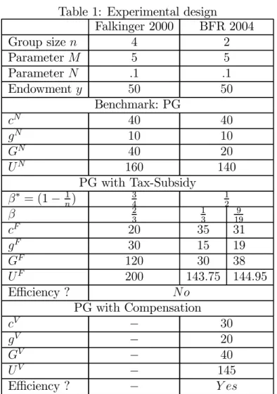
con-Table 1: Experimental design Falkinger 2000 BFR 2004 Group size n 4 2 Parameter M 5 5 Parameter N .1 .1 Endowment y 50 50 Benchmark: PG cN ₄₀ ₄₀ gN ₁₀ ₁₀ GN ₄₀ ₂₀ UN 160 140 PG with Tax-Subsidy β∗ = (1₋ _n1) 3₄ 1₂ β 2 3 1 3 9 19 cF 20 35 31 gF ₃₀ ₁₅ ₁₉ GF ₁₂₀ ₃₀ ₃₈ UF ₂₀₀ _143.75 _144.95 Eﬃciency ? N o PG with Compensation cV − 30 gV ₋ 20 GV ₋ 40 UV − 145 Eﬃciency ? ₋ Y es

(10)

texts. Here we want to apply the two mechanisms to the same context in order to compare their performance.

In the setting of a public good game, both the tax-subsidy and the com-pensation mechanism act on the budget constraint. We recall that in the voluntary provision game the budget constraint is:

ci = yi− gi (2)

In the tax-subsidy mechanism the budget constraint is:

ci = yi− gi+ β(gi− gj) (3)

and in the compensation mechanism it is :

ci = yi− gi+ sjgi− sigj (4)

So we can express the diﬀerence among these three situations in terms of how ci, the contribution to the private good, is calculated.

This aspect made the design of the two experiments we ran to investigate the performance of the two mechanims quite straightforward, as we could keep the same instructions, applying changes only for the way the contribu-tion to the private good was calculated. This facilitated both communicacontribu-tion to the subjects and their understanding of the consequences of their choice in the two treatments they played4.

Falkinger et al. (2000) test the practical tractability and effectiveness of the Falkinger mechanism in the same kind of quadratic games, but with dif-ferent group size, different preferences and different tax-subsidy parameters. Table 1 describes both the experimental game used by Falkinger et al. (2000) - this is referred to as C4 and M4 in their paper - and our modiÞcation. We consider the same parameters for the payoff function, but we deal with only one group size, namely two players. We consider two different values for the parameter β, as we explain more in detail in what follows.

In each experiment participants play two games: a control game, with no mechanism for twenty rounds, and a second game with either mechanism for other twenty rounds.

Thirty subjects took part in the experiment on the compensation mech-anism and Þfty-four subjects took part in the experiment on the tax-subsidy

4_{The set of instructions for the tax subsidy game with β =} 9

19 is included in the

(11)

mechanism (thirty subjects with a parameter β = 9

19 and twenty-four

sub-jects with β = 1₃). We conducted three sessions of each experiment.

Participants were divided into groups with two members each and were informed that they would play against the same opponent in the experiment but would never learn with whom they formed a group. The instructions were read aloud to subjects, who, before playing the game at the computer, had to Þll in a questionnaire to check their understanding of the instructions. Each participant received 50 points as initial endowment and had to de-cide how to allocate this initial endowment between two activities, one bene-Þcial to both players in the same group (activity A) and the other benebene-Þcial only to the donor (activity B). Their decision would have consequences in terms of income earned from both activities. Income from activity A would result from the sum of both group members’ contributions to A, whereas income from activity B would result from the following formula:

Income from B = 5 × contribution to B − µ

1 20

¶

× (contribution to B)2 (5) Subjects did not need to do any calculations as they were provided with a table listing the level of income from activity B corresponding to any possible value of the contribution to B that the subject could make, from zero to 50. The table also listed the income change if activity B increased by one unit and the income change if activity A increased by one unit, in order to make clear how income changed after an additional unit of contribution to either activity.

Total income would result from the sum of income from activity B and income from activity A. This would give each subject a payoﬀ which is derived from the utility function we used in the section 2:

Ui(ci, G) = Mici − 1 2Nic 2 i + G (6) with Mi = M = 5, and Ni = N = 0.1.

The total points scored at the end of each experiment were converted into pounds and added to the fee of £ 2.50 which each participant received for showing up. The average payment was £ 10.00. Each experiment lasted two hours.

(12)

The software z-tree has been used for programming the experiments. In the two experiments the payoﬀ was the same for all the subjects in both treatments. The only change between the control treatment and the mechanism treatments was the way we calculated the total contribution to activity B.

In the control game subjects were asked to decide how many points they wanted to contribute to activity A. Their choice would automatically de-termine the contribution to B, and income from both activities would be calculated by the software. At the end of each period subjects were informed about the contribution of the other group member to activity A, their in-come from activity A and their inin-come from activity B. From a theoretical point of view, subjects participate to a 20-round repeated game of com-plete information, where the stage game admits a unique Nash equilibrium (gi, ci) = (10, 40), and where the subgame perfect Nash equilibrium of the

total game is made of 20 repetitions of the static Nash equilibrium.

In the tax-subsidy game we varied the value of the mechanism parameter β. We set it to a value below the optimal level β∗ = 1₂, that otherwise would have given multiple solutions to the game. From many voluntary contribution experiments we know that subjects, on average, overcontribute relative to the predicted equilibrium, so we were conÞdent of staying in the predicted equi-librium despite a slightly lower reward/penalty for any discrepancy between players’ contribution to the public good. We tried two diﬀerent values, and Þrst set β equal to 1₃ and then to ₁₉9, a value closer to the optimal one.

The only diﬀerence between the control game and the mechanism game was the way the contribution to activity B was calculated. In the tax-subsidy game the contribution to activity B was split into a direct contribution and an indirect contribution. The direct contribution was as in the control group, corresponding to what remained of the initial endowment after the subject had decided how many points to allocate to activity A. This would be repres-ented by yi− gi in expression (3) The indirect contribution was the diﬀerence

between the two group members’ contribution to activity A multiplied by 1₃ or ₁₉9, which would correspond to β(gi−gj)in expression (3). The same table

as in the control game could be used to work out the income from activity B for each level of the (total) contribution to B.

Theoretically, this is again a repeated game of complete information, where the subgame perfect Nash equilibrium is the repetition of the unique

(13)

static Nash equilibrium, i.e. (ci, gi) = (15, 35) for β equal to1₃ and (ci, gi) =

(19, 31) for β equal to₁₉9 .

In the compensation mechanism treatment, subjects were given the option to oﬀer a rate at which to support the other group member in order to encourage him to contribute to activity A. Once players had decided on the rate of support they had to choose how many points to allocate to activity A. In this mechanism treatment the total contribution to activity B was split into a direct contribution and the diﬀerence between the other group member’s contribution to one’s activity B and one’s own contribution to the other group member’s activity B. As before, the direct contribution was what remained of the initial endowment once the subjects had decided how many points to allocate to activity A. This would correspond to the term yi− gi

in equation (4). The other group member’s contribution to one’s activity B was calculated by multiplying the rate at which the other group member was willing to support his opponent times his opponent’s contribution to activity A. This corresponds to the term sjgi in equation (4). One’s contribution to

the other group member’s activity B was calculated by multiplying one’s rate of support times the other group member’s contribution to activity A. This corresponds to the term sigj in equation (4). As in the previous experiment

the same table as in the control game could be used to work out the income from activity B for each level of the (total) contribution to B.

A subgame perfect equilibrium of each two-stage game is a contribution of 20 to activity A and 30 to activity B, (gi, ci) = (20, 30). And a subgame

perfect Nash equilibrium over the 20 rounds is the repetition of this two-stage equilibrium.

In the following section we examine the impact of the mechanisms by comparing the observed behaviour over time in the Control and in the Treat-ment.

4 Experimental results of the two experiments

This section evaluates the effectiveness of both incentive schemes. We offer descriptive statistics of the contributions to the public good, results of tests on the effects of the treatments, and we show plots of time series of contri-butions. Throughout this section, the reported statistic is the ”contribution to the public good by pairs of subjects”.

(14)

4.1 Contributions to the public good

Table 2 reports on the descriptive statistic ”average sum of contributions”, for both parts of each experiment. Data from play of the game by the pairs of subjects are organized into blocks of Þve rounds. In each control of each experiment, the levels of contributions are high. Subjects start at a very high level, close to the Pareto eﬃcient level of 40, and although play moves towards Nash equilibrium, there is still substantial overcontribution after a few rounds of play. In the last Þve rounds, the observed average level is about 20% higher than predicted by theory.

As for the treatment sessions:

1. There is a rapid, large shift in the level of contributions after the mech-anisms are introduced. The tax-subsidy mechanism with β = 1₃ pro-duces a jump from around 25 in the last Þve rounds of the control to around 38 in the Þrst Þve rounds of the treatment. With β = ₁₉9, the mechanism increases the level from 23 in the last Þve rounds of the control to around 52 of the Þrst Þve rounds of the treatment. For the compensation mechanism, there is a jump from around 24 to around 37.

2. For all blocks, the contributions are higher under the tax-subsidy treat-ment with high value of β than under the compensation treattreat-ment. 3. For the last three blocks, the contributions are higher under the

com-pensation treatment than under the tax-subsidy treatment with low value of β, which itself is characterized by higher contributions than under the control.

4. The sum of contributions under the tax-subsidy mechanism is predicted accurately, after some adjustment,

5. whereas the sum of contributions under the compensation mechanism is predicted inaccurately, even after some adjustment.

4.2 Average contribution and conÞdence bounds over

time

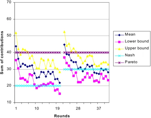
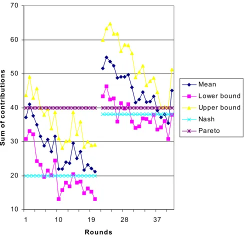
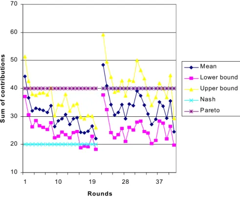
Figures 1, 2 and 3 report the time series of the contributions. The Þgures show the sum of contributions to the public good averaged over either all control groups or all treatment groups. In addition to the average of the

(15)

Table 2: Experimental results: Sum of contributions

Experiment 1a Experiment 1b Experiment 2

Control Tax-Subsidy Control Tax-Subsidy Control Compen-β = 1 3 β = 9 19 sation Nash 20 30 20 38 20 40 Pareto 40 Rounds 1-5 35.50 38.37 36.48 52.21 35.65 37.07 Rounds 6-10 29.58 30.88 27.99 47.05 30.51 34.13 Rounds 11-15 27.18 30.37 24.83 42.75 29.16 31.75 Rounds 16-20 25.13 29.00 23.03 38.97 24.36 31.65

sum of contributions, the Þgures show the 95% conÞdence interval bounds for the average group sums. To calculate the conÞdence intervals, we used the method of bootstrapping (with N = 1000).

We observe movement towards Nash equilibrium under all controls, fast convergence to equilibrium under the treatment with tax-subsidy parameter β = 1₃ and slower convergence to equilibrium under the treatment with β =

9

19. In contrast, we do not observe movement towards the predicted value

(16)

10 20 30 40 50 60 70 1 10 19 28 37 Rounds S u m of c ont ri b u ti o n s M ean Lower bound Upper bound Nash P areto

Figure 1: Sum of contributions and conÞdence bounds; Control and Tax Subsidy mechanism with beta = 1/3

(17)

10 20 30 40 50 60 70 1 10 19 28 37 Rounds S u m of c o nt ri b u ti o n s Mean Lower bound Upper bound Nash Pareto

Figure 2: Sum of contributions and conÞdence bounds; Control and Tax-Subsidy mechanism with beta = 9/19

(18)

10 20 30 40 50 60 70 1 10 19 28 37 Rounds S u m o f c o nt ri bu ti o n s Mean Lower bound Upper bound Nash Pareto

Figure 3: Sum of contributions and conÞdence bounds; Control and Com-pensation mechanism.

(19)

4.3 Nonparametric tests

This subsection Þrst compares the contributions under the controls in exper-iments 1a and 1b with the contributions under the control in experiment 2. We conclude that the contributions are similar in the experiments. Then, we assess the eﬀect of each treatment. That is, we compare the contributions under the control with the contributions under the corresponding treatment. Lastly, we compare the contributions under both treatments.

Do we observe similar levels of contributions in the controls? The average sum of contributions in control sessions from experiments 1a and 1b are 29.35 and 28.08, respectively. The average sum of contributions in experiment 2 is 29.92. We use a two-sample Wilcoxon rank-sum (Mann-Whitney) test. The null hypothesis is that the median of the diﬀerence of the average sum of contributions under the control in experiments 1a and 1b, denoted ¯GN

1 , and

the average sum of contributions under the control in experiment 2, denoted ¯

GN

2 , is zero5.

The results show that the medians are not statistically diﬀerent at any level below .59 (with low value of β) and below 0.18 (with high value of β). We conclude that there is no diﬀerence between either control of experiment 1 and the control of experiment 26_.

Above, the unit of observation was the average of the sum of contribu-tions. That is, with twenty rounds, we calculate twenty statistics i.e. twenty average sums of contributions. Now, let the unit of observation be the sum of contributions of each pair. For instance, with twenty rounds and twelve pairs, we calculate two hundred forty statistics i.e. two hundred forty sums of contributions7_{. With the two-sample Wilcoxon rank-sum (Mann-Whitney)}

test, Þrst, we Þnd that [P rob > |z|] = .28 when we compare the control of experiment 1 with low value of β with the control of experiment 2; second, we Þnd that [P rob > |z|] = .05 when we compare the control of experiment 1 with high value of β with the control of experiment 2 and, Þnally, we Þnd that [P rob > |z|] = .24 when we compare the controls of experiment 1. We conÞrm our Þndings and we conclude that there is no diﬀerence between the controls.

5_{The test use as inputs ¯}_GN

1, the contributions summed over all pairs for each round t =

1, 2, ..., 20 and ¯GN

2, the contributions summed over all pairs for each round t = 1, 2, ..., 20.

6_{The medians of the controls of experiment 1 are not statistically diﬀerent at any level}

below 0.29. There is no diﬀerence between those controls, too.

7_{The test use as inputs G}N

1 of each pair for each round t = 1, 2, ..., 20 and GN2 of each

(20)

4.3.1 Does the tax-subsidy mechanism change agents’ behavior? For the chosen value of the tax-subsidy parameter β = 1₃, theory predicts a level of the public good equal to 30. The sum of contributions averaged over twelve pairs and twenty rounds is 31.63. In the last Þve rounds, the average sum of contributions is 29.00. The median average sum of contributions in the last Þve rounds is 29.33. We conclude that the observations are very close to equilibrium.

Does the treatment (with β = 1₃)signiÞcantly increase the level of contri-butions? First, we use a Wilcoxon signed-ranks test. The null hypothesis is that the median of the diﬀerence of the average sum of contributions under the control, denoted ¯GN1 , and the average sum of contributions under the

treatment, denoted ¯GF_{, is zero}8_{. The null hypothesis can be rejected at any}

level below .09. We conclude that there is a signiÞcant diﬀerence between control and treatment over all rounds.

Second, we use a bootstrap test9_{. The null hypothesis is that the level of}

the public good is identical in the control and the treatment sessions. Using a 5 % level of signiÞcance, we can reject the hypothesis on data from rounds 11-15 and data from rounds 16-20. More precisely, from the resulting data:

• in rounds 1 − 5, the diﬀerence diﬀerence between the contributions in the treatment and the contribution in the control is 2.87, with a bias of .02, a standard error of 1.62 and a 95% conÞdence interval of [−.31 6.04].

• in rounds 6 − 10, the diﬀerence in contributions is 1.30, with a bias of −.10, a standard error of 1.58 and a 95% conÞdence interval of [−1.80 4.40].

• in rounds 11 − 15, the diﬀerence in contributions is 3.18, with a bias of .00, a standard error of 1.42 and a 95% conÞdence interval of [.39 5.97]. • Þnally, in rounds 16 − 20, the diﬀerence in contributions is 3.87, with a bias of −.02, a standard error of 1.53 and a 95% conÞdence interval of [.86 6.87].

1, 2, ..., 20 and ¯GF, the contributions summed over all pairs for each round t = 1, 2, ..., 20.

1 of each pair and GF of each pair for rounds t = 1, 2, ..., 5

(21)

We conclude that there is a signiÞcant diﬀerence between control and treatment in the last ten rounds.

When the tax-subsidy parameter β equals ₁₉9, theory predicts a level of the public good equal to 38. The sum of contributions averaged over Þfteen pairs and twenty rounds is 45.25. In the last Þve rounds, the average sum of contributions is 38.97. The median average sum of contributions in the last Þve rounds is 38.13. We conclude that the observations are close to equilibrium.

Does the treatment (with β = ₁₉9)signiÞcantly increase the level of contri-butions? First, we use a Wilcoxon signed-ranks test. The null hypothesis is that the median of the diﬀerence of the average sum of contributions under the control, denoted ¯GN

1 , and the average sum of contributions under the

treatment, denoted ¯GF, is zero10. The null hypothesis can be rejected at any reasonable level (P rob > |z| = .00). We conclude that there is a signiÞcant diﬀerence between control and treatment over all rounds.

Second, we use a bootstrap test11_{. The null hypothesis is that the level}

of the public good is identical in the control and the treatment sessions. • in rounds 1 − 5, the diﬀerence between the contributions in the

treat-ment and the contribution in the control is 15.73, with a bias of .21, a standard error of 2.86 and a 95% conÞdence interval of [10.12 21.35]. • In rounds 6 − 10, the diﬀerence in contributions is 19.07, with a bias of

.075, a standard error of 2.60 and a 95% conÞdence interval of [13.97 24.16].

• In rounds 11−15, the diﬀerence in contributions is 17.92, with a bias of −.03, a standard error of 2.40 and a 95% conÞdence interval of [13.21 22.63].

• Lastly, in rounds 16 − 20, the diﬀerence in contributions is 15.95, with a bias of .064, a standard error of 1.95 and a 95% conÞdence interval of [12.11 19.78].

Hence, using a 5% level of signiÞcance, we can reject the hypothesis on data from rounds 1 − 5, 6 − 10, 11 − 15 and 16 − 20.

1, 2, ..., 20 and ¯GF_{, the contributions summed over all pairs for each round t = 1, 2, ..., 20.}

1 of each pair and GF of each pair for rounds t = 1, 2, ..., 5

(22)

We conclude that there is a signiÞcant diﬀerence between control and treatment.

4.3.2 Does the compensation mechanism change agents’ beha-vior?

The predicted level of the public good is 40. The average sum of contributions of Þfteen pairs and twenty rounds is 33.97. In the last Þve rounds, the average sum of contributions is 31.65 and the median average sum of contributions is 33.73.

Does the treatment have an eﬀect? Again, using a Wilcoxon signed-ranks test, the null hypothesis is that the median of the diﬀerence of the average sum of contributions under the control ( ¯GN

2 ) and the average sum of

contributions under the treatment ( ¯GV) is zero12. The results indicate that the medians are not statistically diﬀerent at any level below .22. On this basis, one may conclude that there is only an insigniÞcant diﬀerence between control and treatment over all rounds.

However, a bootstrap test13 _{with a 5% level of signiÞcance rejects the null}

hypothesis that the level of the public good is the same under the control and the treatment on data from the last Þve rounds. SpeciÞcally, we Þnd:

• in rounds 1 − 5, the diﬀerence in contributions is 1.41, with a bias of −.22, a standard error of 2.36 and a 95% conÞdence interval of [−3.23 6.06].

• in rounds 6 − 10, the diﬀerence in contributions is 3.63, with a bias of −.06, a standard error of 2.27 and a 95% conÞdence interval of [−.85 8.10].

• In rounds 11 − 15, the diﬀerence in contributions is 2.59, with a bias of −.02, a standard error of 2.26 and a 95% conÞdence interval of [−1.85 7.02].

• And in rounds 16 − 20, the diﬀerence in contributions is 7.29, with a bias of −.07, a standard error of 2.11 and a 95% conÞdence interval of [3.16 11.42].

Hence, we conclude that there is a signiÞcant diﬀerence between control and treatment in the last Þve rounds.

2, contributions summed over all pairs for each round t =

1, 2, ..., 20 and ¯GV_{, contributions summed over all pairs for each round t = 1, 2, ..., 20.}

1 of each pair and ¯GF of each pair for each round t = 1, 2, ..., 5

(23)

4.3.3 Do the two mechanisms have diﬀerent eﬀects?

Do we observe signiÞcantly diﬀerent levels of contributions in the two types of treatments? The average sum of contributions in the experiment with tax-subsidy parameters β = 1₃ and β = ₁₉9 are respectively 32.15 and 45.25. The average sum of contributions in the experiment with compensation option is 33.65.

We use a two-sample Wilcoxon rank-sum (Mann-Whitney) test. The null hypothesis is that the median of the diﬀerence of the average sum of contributions under the tax-subsidy mechanism, denoted ¯GF_{, and the average}

sum of contributions under compensation mechanism, denoted ¯GV_{, is zero}14_.

The medians of the tax-subsidy mechanism with low value of β and the compensation mechanism are not statistically different at any level below .27. We conclude that there is only an insigniÞcant difference between treatments. The medians of the tax-subsidy mechanism with high value of β and the compensation mechanism are statistically different at any reasonable level ([P rob > |z|] = .00). We conclude that there is difference between treat-ments.

Above, the unit of observation was the average of the sum of contribu-tions. That is, with twenty rounds, we calculate twenty statistics i.e. twenty average sums of contributions. Now, let the unit of observation be the sum of contributions of each pair. For instance, with twenty rounds and twelve pairs, we calculate two hundred forty statistics i.e. two hundred forty sums of con-tributions15. We use the two-sample Wilcoxon rank-sum (Mann-Whitney) test. When we compare the tax-subsidy mechanism with low value of β with the compensation mechanism, we Þnd [P rob > |z|] = .78. When we com-pare the tax-subsidy mechanism with high value of β with the compensation mechanism, we Þnd [P rob > |z|] = .00. We conÞrm our Þndings and we con-clude that there is no diﬀerence between the compensation mechanism and the mechanism with low value of the tax-subsidy parameter whereas there is a diﬀerence between the compensation mechanism and the mechanism with high value of the tax-subsidy parameter.

14_{The test use as inputs ¯}_GF_{, contributions summed over all pairs for each round t =}

1, 2, ..., 20 and ¯GV_{, contributions summed over all pairs for each round t = 1, 2, ..., 20.}

15_{The test use as inputs G}F _{of each pair for each round t = 1, 2, ..., 20 and G}V _{of each}

(24)

4.4 Tentative explanations

Two main experimental Þndings surface, that ought to be explained: i) the clear superiority of the tax-subsidy mechanism in its ability to promote co-operation, ii) subjects’ decisions converge to the predicted values in the tax-subsidy treatment, whereas there is a lack of convergence under the com-pensation treatment.

It is tempting to see the Þrst phenomenon as a conÞrmation of the "crowding out" effect mentioned in the introduction, i.e. the compensa-tion is less efficient because it deters any role for social norms in favor of cooperation, while substituting real but weak incentives to depart from free-riding. It should also be mentioned that subjects in the laboratory found the compensation mechanism environment harder to understand, even in this highly stylised public good problem, and the difficulty to devise their optimal strategy is a serious candidate for explaining the phenomenon. Besides, those two explanations might be strongly related, in which case the superiority of "coercion" solutions might be essentially due to their simplicity.

The relative lack of simplicity might also explain why the liberal solution does not seem to converge. Another explanation has to do with the role played by supermodularity properties in learning. Those properties theoret-ically ensure convergence to the equilibrium under various learning dynamics (see Chen (2003)). Experimentally it has been conÞrmed that modular or near supermodular mechanism, like Falkinger mechanism16_{, have good}

con-vergence properties. The absence or presence of the supermodularity prop-erty for the public good game with the compensation mechanism is an open question. The lack of convergence observed in the laboratory suggests that this property might be lacking.

5 Conclusion

This paper investigates experimentally the relative performance of the tax-subsidy mechanism over the compensation mechanism in a public good prob-lem. To summarize, it provides experimental supportive evidence that: i) the two mechanisms do change agents behaviours in the direction of increased cooperation, ii) for a low value of the tax-subsidy parameter β = 1/3, the changes resulting from the two mechanisms are not signiÞcantly diﬀerent, iii) however, with a higher value β = 9/19, closer to the one required for

(25)

efficiency, the mechanisms do have different effects, iv) furthermore, with the tax-subsidy mechanism, theoretical predictions are more accurate and there is convergence, whereas with the compensation mechanism variability is important and convergence is problematic. Points ii), iii) and iv) make a case in favour of the tax-subsidy mechanism: indeed, even with a choice of β which is somehow below its "efficient" level, the performance of the mechanism in terms of promoting cooperation is comparable with that of the compensation mechanism; besides the prediction under the tax-subsidy treatment are more reliable.

The lack of convergence under the compensation treatment might be due to a learning problem. This mechanism is relatively more complex than the tax-subsidy mechanism: there are two decision variables, and backward induction is required. In this respect, adding more rounds would be helpful.

References

[1] Andreoni, J. and H. Varian, 1999, ”Pre-play Contracting in the Prison-ers’ Dilemma”, Proceedings of the National Academy of Science, USA, (96), 10933-10938.

[2] Attiyeh G., R. Franciosi and M. Isaac, 2000, ”Experiment with the pivot process for providing public goods”, Public choice, 102, 95-114.

[3] Chen Y. and C.R. Plott, 1996, ”The Groves-Ledyard mechanism: an ex-perimental study of institutional design”, Journal of Public Economics, 59, 335-364.

[4] Chen Y., 2000, ”Dynamic stability of Nash-eﬃcient public goods mech-anisms: reconciling theory and experiments”, working paper.

[5] Chen Y. and F.-F. Tang, 1998, ”Learning and incentive compatible mechanisms for public goods provision: an experimental study”, Journal of Political Economy, 106-3, 633-662.

[6] Chen Y. and R.S. Gazzale, 2003, ”When does learning in games generates convergence to Nash equilibria? The role of supermod-ularity in an experimental setting”, working paper accessible at http://www.si.umich.edu/ yanchen/papers/comp20030804.pdf.

(26)

[7] Danziger L. and A. Schnytzer, 1991, ”Implementing the Lindahl voluntary-exchange mechanism”, European Journal of Political Eco-nomy, 7, 55-64.

[8] Falkinger J., 1996, ”Eﬃcient private provision of public goods by reward-ing deviations from average”, Journal of Public Economics, 62, 413-422. [9] Falkinger J., Fehr E., Gachter S. and Winter-Ebmer R., 2000, “A Simple Mechanism for the Eﬃcient Provision of Public Goods: Experimental Evidence”, American Economic Review, 90(1): 247-264.

[10] Guttman J.M., 1978, ”Understanding collective actions: matching beha-vior”, American Economic Review, papers and proceedings 68, 251-255. [11] Guttman J.M., 1985, ”Collective action and the supply of campaign

funds”, European Journal of Political Economy, 1, 221-241.

[12] Guttman J.M., 1987, ”A non-Cournot model of voluntary collective ac-tion”, Economica, 54, 1-19.

[13] Harstad R.M. and M. Marese, 1981, ”Implementation of mechanism by processes: public good allocation experiments”, Journal of Economic Behavior and organization, 2, 129-151.

[14] Harstad R.M. and M. Marese, 1982, ”Behavioral explanations of eﬃcient public good allocations”, Journal of Public Economics, 19, 367-383. [15] Keser C., 1996, ”Voluntary contributions to a public good when partial

contribution is a dominant strategy”, Economics Letters, 50, 359-366. [16] Moore J. and R. Repullo, 1988, ”Subgame perfect implementation”,

Econometrica, 56(5), 1191-1220.

[17] Ostrom, E., 2000, "Collective action and the evolution of social norms", Journal of Economic Perspectives, 14(3), 137-158.

[18] Sefton M. and R. Steinberg, 1996, ”Reward structures in public goods experiments”, Journal of Public Economics, 61(2), 263-288.

[19] Varian Hal, 1994a, “A Solution to the Problem of Externalities When Agents Are Well-Informed”, American Economic Review, 84, 1278-1293. [20] Varian Hal, 1994b, “Sequential contributions to public goods”, Journal

(27)

[21] Willinger M. and A. Ziegelmeyer, 1999, ”Framing and cooperation in public good games: an experiment with an interior solution”, Economics Letters, 65, 323-328.

(28)

6 Appendix

Instructions for the tax-subsidy experiment

with beta = 9/19.

Instructions (Control)

You are now taking part in an experiment which has been Þnanced by the Leverhulme Centre for Market and Public Organisation at the Department of Economics, University of Bristol. If you read the following instructions carefully, you can, depending on your decisions, earn a considerable amount of money in addition to the £2.50 you will received anyway. It is therefroe very important that you read these instructions with care. At the end of the experiment all earnings will be added and paid to you in cash.

During the experiment your entire earnings will be calculated in "Points". At the end of the experiment the total amount of Points you have earned will be converted to Pounds at the following rate:

100 Points = $ 0.125

In this experiment there are 12 participants, which are divided into 6 groups with 2 members each. Except us, i.e., the experimenters, no one knows the group composition.

The experiment is divided into 20 periods. In each period you have to make a decision that you have to enter into the computer. During these 20 periods the group composition stays the same. You are, therefore, remaining with the same people in a group for 20 periods, but you will never learn with whom you formed a group.

The instructions which we have distributed to you, are solely for your private information. It is prohibited to communicate with the other parti-cipants during the experiment. Should you have any questions, please ask us. If you violate this rule, we will have to exclude you from the experiment and from all payments.

(29)

At the beginning of each period each participant gets 50 points, which in the following we call endowment. Your task is to make a decision how to use your endowment. There are two activities for which you can use your endowment: activity A and activity B. These activities result in diﬀerent incomes which we will explain in more detail below.

At the beginning of each period the following screen will appear: [Insert screen shot of decision screen, Control]

You have to decide how many points you want to contribute to activity A by typing a number between 0 and 50 in the input Þeld. This Þeld can be reached by clicking it with the mouse. As soon as you have decided how many points to contribute to activity A, you have also decided how much your contribution to activity B is, namely, (50 - your contribution to activity A) points.

The current period appears in the top left corner of the screen. In the top right corner you can see how many more seconds remain for you to decide on the distribution of your points. Your decision must be made before the time displayed is 0 seconds. After you have inserted your contribution you have to press the OK-button (with the help of the mouse). As soon as you have pressed the OK-button you cannot revise your decision for the current period anymore.

After all members of your group have made their decision, the following income screen will appear.

[Insert screen shot of income screen 1, Control]

Besides the period and the remaining time for watching the income screen, the income screen shows the following entries, which we will explain in detail below.

1. Your contribution to activity A 2. Your income from activity A 3. Your contribution to activity B 4. Your income from activity B 5. Your total income in this period

(30)

In the following we will explain these items in detail.

1. Your contribution to activity A:

Here your contribution to activity A as you have inserted it previously is listed.

2. Your income from activity A:

Your income from activity A is your contribution to activity A plus the other group member’s contribution to activity A.

Income from activity A = sum of contributions of both group members to activity A

The income of the other group member from activity A is calculated according to the same formula, i.e., each group member has the same income from activity A. If, for example, the sum of contributions of both group members is 60 points, you and the other group member receive an income of 60 points from activity A. If both group members together invest 10 points in activity A, you and the other group member each receive an income of 10 points.

Therefore, each point that you contribute to activity A, increases your income by 1 point. However, this also increases the income of the other group member by 1 point, such that the total income of the group increases by 2 × 1 = 2 points. Hence, through your contribution to activity A the other group member earns something. In turn, it also holds that you earn something from the contribution of the other group member.

3. Your contribution to activity B:

Your contribution to activity B is the diﬀerence between your endowment of 50 points and your contribution to activity A:

Your contribution to activity B = 50 - contribution to activity A

4. Your income from activity B:

An important diﬀerence between the contributions to activity A and activity B is that from your contribution to activity A the other group mem-ber earns something in the same way, whereas from your contribution to

(31)

activity B only you earn something. In turn, it also holds that you earn in the same way from the contribution of the other group member to activity A, while you earn nothing from the contribution of the other group members to activity B. The income of each group member from his contributions to activity B is calculated according to the following formula:

Income from activity B = 5_{×contribution to activity B}

- (₂₀1 )_{×(contribution to activity B)}2

The income from activity B will be calculated for both group members according to the same formula. In the Table your income from activity B is indicated for each level of your contribution to activity B. If your con-tribution to activity B is 0, for example, then your income from activity B is 0 (see Table). If your contribution is 25, then you will earn an income of 93.75 points from activity B (see Table). If your contribution is 50, then you will earn an income from activity B of 125.

Your income from activity B depends therefore on your contribution to activity B. The other group member earns - in contrast to activity A - nothing from your contribution to activity B.

In the enclosed Table not only your income from the contribution to activity B is listed, but also the income change, if activity B increases by 1 unit, as well as the income change, if activity A increases by 1 unit. As you see (and as already explained above under ”Income from activity A”) your income from activity A increases always exactly by 1 unit for each additional point you or the other group member contributes to activity A. The income change in activity B, however, is not constant. The income change is smaller, the larger your contribution to activity B already is. Therefore when your contribution to activity B is low (because your contribution to activity A is high) an additional contribution to activity B generates a relatively large additional income from activity B. If, in contrast, your contribution to activity B is high (because your contribution to activity A is low) an additional contribution to activity B generates a relatively low additional income from activity B.

5. Your total income in a period:

The total income (in points) in a period is

Income from activity A + income from activity B

At the end of the experiment the total incomes of all periods will be added up and exchanged into Pounds.

(32)

Control questionnaire:

Please answer all questions. Their purpose is only to enhance your un-derstanding. Please always write down the whole calculation. If you have questions, please ask us!

1. Each group member is endowed with 50 points. Assume that nobody (including you) contributes anything to activity A. What is

Your contribution to activity B? ... Your income from activity A? ... Your income from activity B? ... Your total income in this period? ...

2. Assume that the other group member contributes nothing to activity A. You contribute 10 points. What is

3. Each group member is endowed with 50 points. Assume that each group member (including you) contributes 50 points to activity A. What is

4. Assume that the other group member contributes 50 points to activity A. You contribute 40 points to activity A. What is

(33)

Instructions (Falkinger)

We will repeat the experiment for 20 periods. There is one change that concerns the calculation of the contribution to activity B. Your contribution to activity B consists now of a direct contribution to activity B as well as an INDIRECT contribution to activity B. The course of the experiment is exactly the same as before.

As previously you have to determine in the decision screen your contribu-tion to activity A. In each period, you have again 50 points at your disposal. After you have made your decision, the following income screen will appear:

[Insert income screen, Falkinger]

On the income screen you can see the following entries which we will explain in detail below.

1. Your contribution to activity A

2. Contribution of the OTHER group member to activity A 3. Your income from activity A

4. Your direct contribution to activity B 5. Your INDIRECT contribution to activity B 6. Your total contribution to activity B

7. Your income from activity B 8. Your total income in this period

In the following we will explain these items in detail.

1. Your contribution to activity A:

Here your contribution to activity A as you have inserted it previously is listed.

2. Contribution of the OTHER group member to

activity A:

(34)

If you add the contribution of the OTHER group member to your con-tribution to activity A, you will get the sum of concon-tributions of both group members to activity A.

3. Your income from activity A:

As previously, your income from activity A is your contribution to activity A plus the other group member’s contribution to activity A.

Income from activity A = sum of contributions of both group members to activity A

Therefore, each point that you contribute to activity A, increases your income by 1 point. However, this also increases the income of the other group member by 1 point, such that the total income of the group increases by 2 × 1 = 2 points. Hence, through your contribution to activity A the other group member earns something. In turn, it also holds that you earn something from the contribution of the other group member to activity A.

4. Your direct contribution to activity B:

Your direct contribution to activity B is the diﬀerence between your en-dowment of 50 points and your contribution to activity A:

Your contribution to activity B = 50 - contribution to activity A

This direct contribution therefore corresponds to the contribution to activity B in the previous experiment.

5. Your INDIRECT contribution to activity B:

Your indirect contribution is now the decisive change in the new experi-ment. Your indirect contribution to activity B depends on the contribution made by both you and your group member to activity A (!). The indirect contribution is calculated as follows:

Your INDIRECT contribution to activity B = [Your contribu-tion to activity A minus the contribucontribu-tion of the OTHER group member to activity A]_×(₁₉9)

For example, if you have contributed 21 points to activity A and the other group member has contributed 40 points, then your indirect contribution is

(35)

[21_{− 40] ×} 9

19 =−19 × 9

19 =−9. Your indirect contribution is then negative.

In turn, if you have contributed 40 points to activity A and the other group member has invested 21 points, then your indirect contribution is positive and amounts to [40 − 21] × 9

19 = 9 in this case.

In general the following holds: if your contribution to activity A has been larger than the contribution of the OTHER group member, then your indirect contribution to activity B is positive. If you have contributed less to activity A than the other group member, then your indirect contribution to activity B is negative. If both members contribute the same amount to activity A, then your indirect contribution is zero. The indirect contribution is calculated according to the same formula for both group members.

6. Your total contribution to activity B

The total contribution to activity B is the sum of the direct and the indirect contribution to activity B:

Total contribution to activity B

= direct contribution + INDIRECT contribution = (50 - contribution to activity A)

+ (your contribution to activity A minus

the contribution of the OTHER group member to activity A)×(199)

How many points you contribute eventually to activity B depends not only on the direct contribution to activity B, but also on how much you have invested relative to the other group member in activity A. Each of your point above the contribution of the other group member, increases your INDIR-ECT contribution to activity B by (₁₉9)-points, while each point below the contribution of the other group member decreases your INDIRECT contri-bution by (₁₉9)-points.

At the back of the Table that you have received, the relationships are summarized schematically. Each point that you invest in activity A increases your contribution to activity A by 1 point and decreases the direct contri-bution to B by 1 point. However, this also increases your contricontri-bution to activity A relative to the other group member and therefore also your IN-DIRECT contribution to B increases by ₁₉9. Each additional point for activity A therefore decreases the total contribution to B not by 1 point, but only by 10₁₉-point.

This is the decisive diﬀerence to the previous experiment. In the previous experiment, 1 additional point to activity A resulted in a decrease of your

(36)

contribution to activity B by exactly 1 point. In the new experiment, one additional point for activity A leads to a decrease of the total amount activity B by 10₁₉.

If the other group member increases his contribution to activity A by one point, your income from activity A increases by 1 point (see the lower part of the enclosed schematic overview). However, this also leads to a decrease of your indirect contribution to activity B by 9

19-points since now the other

member contributes relatively more to activity A. 7. Your income from activity B:

The income from activity B is calculated according to the same formula as previously, namely

Income from activity B = 5_{×(total contribution to activity B)} - (₂₀1 )_{×(total contribution to activity B)}2 Recall that the total contribution to activity B equals the direct plus

indirect contribution to activity B.

In the previous experiment, the total contribution to activity B corres-ponded to the contribution to activity B. Now there is also the indirect contribution which depends on the contribution of the other group member to activity A. The only change therefore is in the composition of the total contribution to activity B, not the formula itself. Therefore, the enclosed table which you have already used in the previous experiment is still valid.

Your income from activity B depends therefore on your total contributions to activity B. As previously, the other group member - in contrast to activity A - earn nothing from your direct or indirect contribution to activity B.

8. Your total income in a period: The total income (in points) in a period is

Income from activity A + income from activity B

At the end of the experiment the total incomes of all periods will be added up and exchanged into Pounds.

(37)

Control questionnaire:

Please answer all questions. Their purpose is only to enhance your un-derstanding. Please always write down the whole calculation. If you have questions, please ask us!

1. Each group member is endowed with 50 points. Assume that nobody (including you) contributes anything to activity A. What is

Your direct contribution to activity B? ... Your indirect contribution to activity B? ... Your total contribution to activity B? ... Your income from activity A? ... Your income from activity B? ... Your total income in this period? ...

2. Assume that the other group member contributes nothing to activity A. You contribute 19 points. What is

3. Each group member is endowed with 50 points. Assume that each group member (including you) contributes 50 points to activity A. What is

4. Assume that the other group member contributes 50 points to activity A. You contribute 31 points to activity A. What is

(38)

1 additional token by you to activity A

. ↓ &

increases contribution decreases the direct contribution increases the INDIRECT to activity A by 1 to activity B by 1 contribution to activity B

(your income also by ₁₉9-token

increases by 1 point) _& _.

decreases the total contribution to activity B by 10₁₉-token {generated income change depends on the level of activity B -see Table}

If the other group member contributes an additional token to activity A

. &

increases contribution to decreases your INDIRECT contribution

activity A by 1 and your total contribution to activity B

(increases also your income by ₁₉9-token

by 1 point) (generated income changes depend on the

(39)

Total Your Income Income Total Your Income Income

contribution income change if change if contribution income change if change if

to from activity B activity A to from activity B activity A

activity B activity B increases increases activity B activity B increases increases

by 1 unit by 1 unit by 1 unit by 1 unit by 1 unit

0 0.00 4.95 1.00 26 96.20 2.35 1.00 1 4.95 4.85 1.00 27 98.55 2.25 1.00 2 9.80 4.75 1.00 28 100.80 2.15 1.00 3 14.55 4.65 1.00 29 102.95 2.05 1.00 4 19.20 4.55 1.00 30 105.00 1.95 1.00 5 23.75 4.45 1.00 31 106.95 1.85 1.00 6 28.20 4.35 1.00 32 108.80 1.75 1.00 7 32.55 4.25 1.00 33 110.55 1.65 1.00 8 36.80 4.15 1.00 34 112.20 1.55 1.00 9 40.95 4.05 1.00 35 113.75 1.45 1.00 10 45.00 3.95 1.00 36 115.20 1.35 1.00 11 48.95 3.85 1.00 37 116.55 1.25 1.00 12 52.80 3.75 1.00 38 117.80 1.15 1.00 13 56.55 3.65 1.00 39 118.95 1.05 1.00 14 60.20 3.55 1.00 40 120.00 0.95 1.00 15 63.75 3.45 1.00 41 120.95 0.85 1.00 16 67.20 3.35 1.00 42 121.80 0.75 1.00 17 70.55 3.25 1.00 43 122.55 0.65 1.00 18 73.80 3.15 1.00 44 123.20 0.55 1.00 19 76.95 3.05 1.00 45 123.75 0.45 1.00 20 80.00 2.95 1.00 46 124.20 0.35 1.00 21 82.95 2.85 1.00 47 124.55 0.25 1.00 22 85.80 2.75 1.00 48 124.80 0.15 1.00 23 88.55 2.65 1.00 49 124.95 0.05 1.00 24 91.20 2.55 1.00 50 125.00 -0.05 1.00 25 93.75 2.45 1.00 - - - -1

(40)

(41)

(42)