Gradient boosting techniques for individual loss reserving in non-life insurance

UNIVERSITÉ DU QUÉBEC

À

MONTRÉAL

GRADIENT BOOSTING TECHNIQUES FOR INDIVIDUAL LOSS RESERVING IN NON-LIFE INSURANCE

DISSERTATION PRESENTED

AS PARTIAL REQUIREMENT TO THE MASTERS IN MATHEMATICS

BY

FRANCIS DUVAL

UNIVERSITÉ DU QUÉBEC À MONTRÉAL

TECHNIQUES DE GRADIENT BOOSTING POUR LA

MODÉLISATION DES RÉSERVES INDIVIDUELLES EN

ASSURANCE NON-VIE

MÉMOIRE

PRÉSENTÉ

COMME EXIGENCE PARTIELLE

DE LA MAITRlSE EN MATHÉMATIQUES

PAR

FRANCIS DUVAL

UNIVERSITÉ DU QUÉBEC À MONTRÉAL Service des bibliothèques

Avertissement

La diffusion de ce mémoire se fait dans le respect des droits de son auteur, qui a signé le formulaire Autorisation de reproduire et de diffuser un travail de recherche de cycles supérieurs (SDU-522 - Rév.1 0-2015). Cette autorisation stipule que «conformément à · · l'article 11 du Règlement no 8 des études de cycles supérieurs, [l'auteur] concède à l'Université du Québec à Montréal une licence non exclusive d'utilisation et de publication de la totalité ou d'une partie importante de [son] travail de recherche pour des fins pédagogiques et non commerciales. Plus précisément, [l'auteur] autorise l'Université du Québec à Montréal à reproduire, diffuser, prêter, distribuer ou vendre des copies de [son] travail de recherche à des fins non commerciales sur quelque support que ce soit, y compris l'Internet. Cette licence et cette autorisation n'entraînent pas une renonciation de [la] part [de l'auteur] à [ses] droits moraux ni à [ses] droits de propriété intellectuelle. Sauf entente contraire, [l'auteur] conserve la liberté de diffuser et de commercialiser ou non ce travail dont [il] possède un exemplaire.»

-REMERCIEMENTS

Je souhaite remercier en tout premier lieu mon directeur de recherche, Mathieu Pigeon, qui m'a soutenu et guidé durant mes deux années à la maitrise, plus particulièrement durant la rédaction de ce mémoire. Grâce à lui, il m'a été possible de soumettre mon premier article scientifique. Je salue entre autres sa grande pédagogie, son assiduité ainsi que son professionnalisme. Je remercie également Desjardins Assurances Générales, qui a fournit les données sans lesquelles ce projet ne se serait pas matérialisé. Plus particulièrement, je tiens à remercier Danaïl Davidov, mon superviseur de stage au cours duquel ce projet a débuté. Il m'a donné les outils nécessaires à l'élaboration des modèles, entre autres en m'initiant à l'apprentissage automatique. Finalement, je tiens à remercier ma famille qui m'a soutenu tout au long de mes études à la maitrise.

AVANT-PROPOS

L'idée du projet de recherche présenté dans ce mén1oire a vu le jour lors d'un stage de recherche au sein de Desjardins Assurances Générales achevé à l'été 2017, vers le commencement de ma maîtrise en sciences actuarielles. Ce stage a été financé à parts égales par Desjardins Assurances Générales et par Mitacs, un organisme à but non lucratif visant à stimuler l'innovation et la recherche en établissant des partenariats entre le milieu universitaire et l'industrie. Lors de ce stage, le mandat de trouver un algorithme pern1ettant de prédire les montants futurs à payer pour des réclamations passées m'a été donné.

À

ce mon1ent, les techniques de modélisation des réserves individuelles présentes dans la littérature étaient pour la plupart des méthodes paramétriques. Puisque l'apprentissage statistique était alors un champ d'étude qui produisait des résultats proinetteurs dans divers domaines, j'ai développé un algorithme basé sur une méthode non paramétrique d'apprentissage automatique appelée gradient boosting, qui a été implanté avec succès dans les systèmes de Desjardins Assurances Générales.

L'algorithme de gradient boosting utile au développement du modèle est une boite noire et à l'automne 2017, beaucoup de détails concernant le fonctionnement de cet algorithme m'échappaient. Dans le cadre d'un cours de maîtrise, j'ai donc décidé d'apprendre en détaille fonctionnement de cet algorithme, ce qui a abouti à un document expliquant le fonctionnement du gradient boosting, de l'algorithme random forest ainsi que des arbres de décision, trois techniques connexes appar-tenant à la famille des algorithmes d'apprentissage machine. Ceci n1'a permis d'acquérir une connaissance approfondie du modèle de prédiction des réserves que j'ai développé, ce qui m'a par la suite permis de le perfectionner.

IV

L'été dernier, j'ai eu la chance de présenter les résultats partiels de ce projet au Joint Statistical Meeting tenu à Vancouver, le plus grand rassemblement de statisticiens en Amérique du Nord. Il s'agissait d'une courte présentation de cinq minutes suive d'une séance d'affichage d'une durée d'une heure.

Ce projet a également engendré un article qui a été soumis pour publication au moment d'écrire ces lignes. Cet article a été coécrit par 1noi et Mathieu Pigeon, mon directeur des travaux de recherche à la maîtrise.

Finalement, les résultats finaux de mes travaux effectués à la maitrise ont été présentés au Congrès annuel 2019 à Calgary de la Société statistique du Canada.

CONTENTS

LIST OF TABLES . v1

LIST OF FIGURES vii

RÉSUMÉ . . viii

ABSTRACT 1x

INTRODUCTION 1

CHAPTER I RESERVING PROBLEM SETTING 4

CHAPTER II CLASSICAL MODELS FOR LOSS RESERVING . 9

2.1

Chain-ladder Algorithm and Mack's Model . 9

2.2

Generalized Linear Models . . . . . . . .

12

CHAPTER III STATISTICAL LEARNING AND GRADIENT BOOSTING

15

3.1

Supervised Machine Learning

16

3.2

Gradient Boosting

19

3.2.1

TreeBoost .

24

3.2.2

Regularization

28

3.3

Gradient Boosting for Loss Reserving .

29

CHAPTER IV ANALYSIS.

31

4.1

Data . . . .

31

4.2

Covariates .

35

4.3

liaining of

X G B

oost mo dels .

37

4.4

Results . . . .

45

CONCLUSION ..

58

LIST OF TABLES

Table Page

4.1.1 Comparison of complete set of claimants (

S)

and set of claimants from accident years 2004-2010

(S7 ).

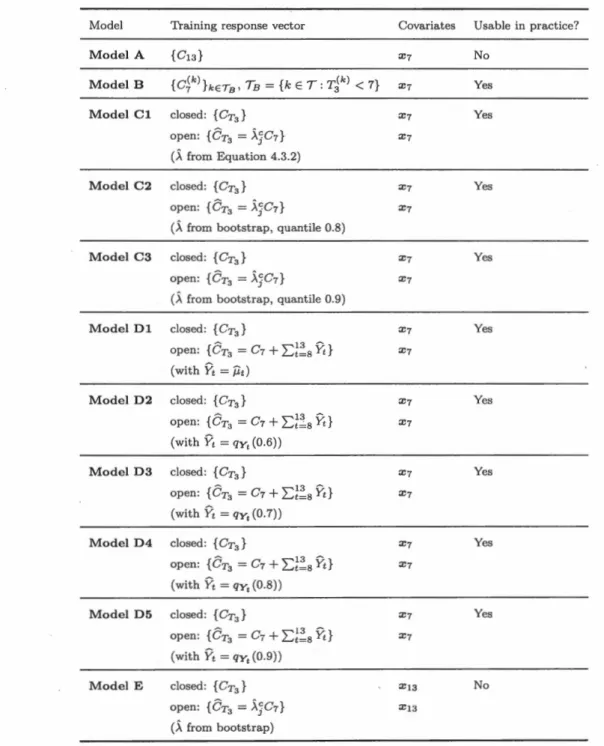
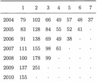
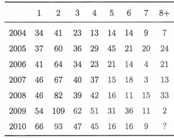
%of open daims is on Decem-ber 31st 2016. . . . . . . . . 36 4.1.2 Details about training and validation datasets. 36 4.2.1 Covariates used in the models. . . . . . . . 37 4.3.1 Main specifications of XGBoost models. Unless otherwise stated,

we have k ET. . . . . . . . . . . . . . . . . . . . . 44 4.4.1 Training increment al run-off triangle (in $100,000). 45 4.4.2 Validation incrementa! run-off triangle (in $.100,000). 46 4.4.3 Prediction results for collective approaches. . . . . . . 48 4.4.4 Prediction results for individual generalized linear models using

co-variates. . . . . . . . . . . . . . . . . . . 52 4.4.5 Prediction results for individual approaches using covariates. 53

LIST OF FIGURES

Figure Page

1.0.1 Development of the daim k. 5

4.1.1 N umber of cl aimants per daim. 33

4.1.2 Distribution of final incurred by accident years (on a base 10 log

sc ale). The first quartile is equal to the minimum for all accident

years since many daims close at zero. The average incurred for

each accident year is represented by a dot. 34

4.1.3 Status of daims on December 3Pt 2016. 35

4.3.1 Status of daims on December 31st 2010. 38

4.4.1 Comparison of predictive distributions for collective models. The

observed reserve amount is represented by the vertical dashed line. 48

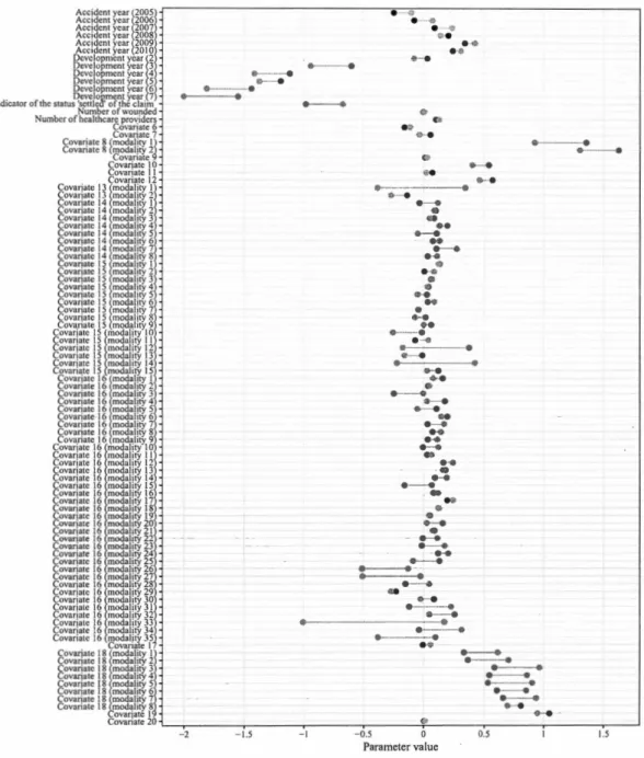
4.4.2 Estimated parameters for quasi-Poisson individual GLM. The black

dots correspond to the out-of-san1ple estimates, as the grey dot are

the in-sample estimates. . . . . . . . . . . . . . . . . . . 51

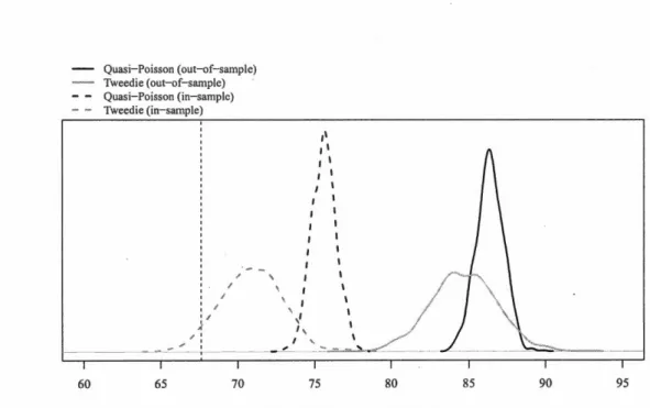
4.4.3 Predictive distributions for in-sample and out-of-sample individual

GLM with covariates. . . . . . . . . . . . . . . . . . . . . . 52

4.4.4 Predictive distributions for XC Boast Madel A, Cl, C2, and C3. 54

4.4.5 Predictive distributions for XGBoost Madel A, Dl, D2, D3 and

D4. . . . . . . . . . . . . . ... . . . . . . . . . . . . 55

4.4.6 Comparison of predictive distributions for Mo del E and Mo del C3. The observed total paid amount is represented by the vertical dashed line. . . . . . . . . . . . . . . . . . . . . . . . . . . . . . 56

RÉSUMÉ

La modélisation fondée sur des données est l'un des sujets de recherche qui pose le plus de défis dans la science actuarielle pour le provisionnement et l'évaluation du risque. La plupart des analyses sont basées sur des données agrégées, mais il est clair aujourd'hui que cette approche ne dit pas tout sur une réclamation et ne décrit pas précisément son évolution. Les approches d'apprentissage statistique en général, et les algorithmes de gradient boosting en particulier, offrent un ensem-ble d'outils qui pourraient aider à évaluer les réserves dans un cadre individuel. Dans ce mémoire, nous comparons certaines techniques agrégées traditionnelles (au niveau du portefeuille) avec des modèles individuels (au niveau de la récla-mation) basés à la fois sur des modèles paramétriques et sur des algorithmes de gradient boosting. Ces modèles individuels utilisent de l'information sur chacun des paiements effectués pour chacune des réclamations du portefeuille, ainsi que sur les caractéristiques de l'assuré. Nous fournissons un exe1nple basé sur un en-semble de données détaillées provenant d'une compagnie d'assurance non-vie et nous discutons de certains points liés aux applications pratiques.

Mots-clé: dssurance non-vie, provisionnement, modélisation prédictive, modèles individuels, gradient boosting

ABSTRACT

Modeling based on data information is one of the most challenging research topics in actuarial science for loss reserving and risk valuation. Most of the analyzes are based on aggregate data but nowadays it is clear that this approach does not tell the whole story about a daim and does not describe precisely its development. Statistical learning approaches in general, and gradient boosting algorithms in particular, offer a set of tools that could help to evalua te loss reserves in an· indi-vidual framework. In this work, we contrast sorne traditional aggregate techniques (portfolio-leve!) with individual models ( claim-level) based on both para1netric models and gradient boosting algorithms. These claim-level models use informa-tion about each of the payments made for each of the daims in the portfolio, as well as characteristics of the insured. We provide an explicit example based on a detailed dataset from a property and casualty insurance company and we discuss sorne points related to practical applications.

Key words: non-life insurance, loss reserving, predictive modeling, individual mod-els, gradient boosting

INTRODUCTION

In its daily practice, a non-life insurance company is subject to a number of sol-veney constraints, e.g., ORSA guidelines in North America and Solvency II in Europe. More specifically, an actuary must predict, with the highest accuracy, fu-ture dailns based on past observations. The difference between the total predicted amount and the total of all amounts already paid represents a reserve that the company must set aside. A substantial part of the actuarial literature is devoted to the modeling, the evaluation and the management of this risk (see [WM08] for an overview of existing methods).

Almost all existing models can be divided into two categories depending on the granularity of the underlying.dataset: individual, or micro-level, approaches when most information on contracts, daims, payments, etc. has been preserved and collective, or macro-level, approaches when an aggregation to sorne extent has been made ( often on an annual basis). The latter have been widely developed by researchers and successfully applied by practitioners for several decades. The former have been studied for few decades but actual use is very rare despite the many advantages of these methods.

The idea of using an individual model - or a structural stochastic description -for daims dates back to the early 1980's with, among others, [BU80], [HA80] and [N086]. The latter has proposed an individual model describing the occurrence, the reporting delay and the severity of each accident separately. The idea was followed by the work of [AR89], [N093A, N099], [HE94], [JE89] and [HA96]. This period was characterized by very limited computing and memory resources

2

as well as by the lack of usable data on individual daims. However, we can find sorne applications in [HA96] and in sorne more technical documents such as (N093B] and (KI94].

Since the beginning of the 2000's, several works have been done - n1ainly in the marked (Poisson) process framework- including the modeling of the depen-dence using copulas [ZZlO], the use of generalized linear mo dels. [LA07], the semi-parametric modeling of certain components [AP14] and [ZZ09], the use of skew-symmetric distributions [PA13], the inclusion of additional information [TM08], etc. Finally, sorne researchers have focused on the comparisons that can be made between individual and collective approaches, often attempting to answer the question "What is the best approach?" (see [HU15], [HI16] or [CP16] for sorne examples).

Nowadays, statisticallearning techniques are widely used in the field of data ana-lytics and may offer non-parametric solutions to daim reserving. These methods give more freedom to the model and often outperform the accuracy of their para-metric counterparts. However, only few non-parapara-metric approaches have been developed using 1nicro-level information. One of them is presented in [WU18], where the number of payments is modeled using regression trees in a discrete time framework. The occurrence of a claim payment is assumed to have a Bernoulli distribution, and the probability is then computed using a regression tree as well as all available characteristics. Other researchers, see [BR17], have also devel-oped a non-parametric approach using a machine learning algorithm known as Extra- Trees, an ensemble of many unpruned regression trees, for loss reserving. In this paper, we propose and analyze an individ ual mo del for loss reserving based on an application of a gradient boosting algorithm. Gradient boosting is a machine learning technique, which combines sequentially many "simple" models called weak

3

learners to form a stronger predictor by optimizing sorne objective function. We apply an algorithm called

XGBoost,

see [CG16], to learn a function to predict the ultimate daim amount of a file using all available information at a given time. This information can be about the daimant as well as the daim itself. We also present and analyze micro-level models belonging to the dass of generalized

linear models (GLM). Based on a detailed dataset from a property and casualty insurance company, we study sorne properties and we compare results obtained from various approaches. More specifically, we show that the approach combining

the

XGBoost

algorithm and a dassical collective madel such as the Mack's madel, has high predictive power and stability. We also propose a method for dealing

with censored data and discuss the presence of dynamic covariates. We believe that the gradient boosting algorithm could be an interesting addition to the range of tools available for actuaries to evaluate the solvency of a portfolio.

In Chapter I, we introduce sorne notation and we present the context of loss reserving from both collective and individual point of view. In this work, our main

objective is to present and to analyze micro-level approaches for loss modeling. We also compare collective and individual approaches. Thus, in Chapter II, we present dassical collective models as well as GLM for individual data. In Chapter III, we present individual models based on machine learning methods, focusing on gradient boosting techniques for regression problems. A case study and sorne numerical analyzes on real data are performed in Chapter IV, and finally, we

CHAPTER I

RESERVING PROBLEM SETTING

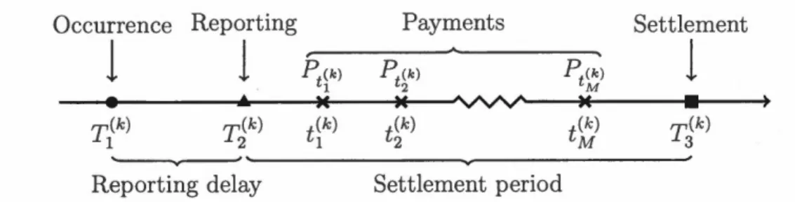
In non-life insurance, a claim always starts by an accident experienced by a policy-holder that may lead to financial damages covered by an insurance contract. We call occurrence point (T1 ) the date on which the accident happens. For sorne situa -tions (bodily injury liability coverage, accident benefits, third party responsibility liability, etc.), a reporting delay is observed between the occurrence point and the notification to the insurer at the reporting point (T_{2 ).} From T₂, the insurer could observe details about the claim, as well as sorne infonnation about the insured, and record a first estimation of the final amount called case estimate. Once the accident is reported to the insurance company, the claim is usually not settled im-mediately: the insurer has to investigate, wait for bills, wait for court judgments, etc. At the reporting point T2 , a series of M random payments

Pt

1, • • • ,

PtM

>

0 made respectively at times _{t 1}

<

.

.. <

tM is therefore triggered, until the claim is closed at the seUlement point (T3 ). It should be noted that it is possible for a claim to close without any payment. All the dates are expressed in number of years sin ce an ad hoc starting point noted by T. Finally, we need a unique index k to distinguish the claims. For instance, T_1(k) is the occurrence date of the claim k,

and t~) is the date of the mth payrrient of this claim. At Figure 1.0.1, we illustrate the development of a claim.

1

1

5

Occurrence Reporting Payments Settlement

1

1

pt(k) pt(k) pt(k)

1

1 2 M

•

...

.E

M

w v

M

•

T(k) 1 y,(k) 2 t(k) 1 t(k) 2 t(k) M T(k) 3 ' - - v - - '

Reporting delay Settlement period

Figure 1.0.1: Development of the claim k.

The evaluation ~ate t* is the moment on which the insurance company wants to evaluate the solvency and compute reserves. At this point, a claim can be classified in three categories:

1. If T{k)

<

t*

<

rJk), the accident has happened but has not yet been reported

to the insurer. It is therefore called an Incurred But Not Reported, or IBNR, accident. For one of those accidents, the insurer does not have specifie information about the accident, but can however use claimant and external information to estimate the reserve.

2. If rJk)

<

t*

<

Tik), the accident has been reported to the insurer but the claim is still not settled, which means the insurer expects to make additional payments to the insured. It is therefore called a Reported But Not Settled,

or RBNS, claim. For one of such daims, the history information as well as claimant and external information can be used to estimate the reserve. 3. If t*

>

Tik), the claim is classified as Settled, or S, and the insurer does not

expect n1ore payment to be done.

for daim k and defined by

C

t (k)- -6 { 0,

I::

pt(k)' {m:t~) ~t} rn

At any evaluation date T{k)

<

t*

<

Tik) and for a daim k, an insurer estimates the cumulative payments amount at the settlement

C~~),

called total paid amount, by ê~~) using all useful information available at t* and denoted by

vi:).

The individual reserve for a daim evaluated at t* is thus given by

R

--(k) _ _{t* -} c ... _T3 Ck) _ eCk) _{t* ·}

For the whole portfolio, the total reserve is the aggregation of all individual re-serves and is given by

K(t*) ... ~ --(k) ltt*

==

~ }tt* '

k=l

w he re K ( t*)

==

1 { k T{ k)

<

t*} 1 is the nun1ber of daims in the portfolio wi th evaluation date t*.

Traditionally, insurance companies aggregate information by accident year and by develop1nent year. Claims with accident year i, i

==

1, ... , I, correspond to all the reported accidents that occurred in the ith year after T, which means all daims k for which i - 1

<

T{k)

< i

is verified. For a daim k, a payment made in development year j is a payment made in the jth year after the occurrence T_1(k),

namely a payment

Pt~)

for which j - 1

<

t~)

- T{k)

<

j.

Example 1.0.1 Let T be January 1st 2004. Claims with accident year 1 are all

the reported accidents th at occurred between t

==

0 and t

==

1, th at is to say between January pt and December 31st 2004, claims with accident year 2 are all reported accidents that occurred between January 1 st and December 31st 2005, etc ..

7

For development years j

=

1, ... ,

J,

we defi ne

where

S~k) =

{m

·

J.- 1

<

t(k) - T(k)

< J.}

J · m 1 '

as the total paid amount for daim k during year j and we define the corresponding

cumulative paid amount as

j

~ik)

=

LY}k).

s=1

Collective approaches group every daim having the sa1ne accident year together to form the aggregate incrementai payment

y ,(k)

J ' i,j=1, ... ,I.

kE{k:i-1<TJk) <i}

Therefore, assuming that I

=

J

=

N, at the evaluation date t* = N an insurer

owns the information, i.e. the run-off triangle

Y(N-1)1 Y(N-1)2

YN1

y1(N-1) Y1N

y2(N-1)

(1.0.1)

where rows represent accident years and columns, development years. It is also

possible to ·write this information in the cumulative form

Cn

c12 c1(N-1) c1N

c21 c22 c2(N-1)

(1.0.2) c(N-1)1 c(N-1)2

8

where Cij

=

2::~=

₁

Yis·

A prediction at time t*

=

N of the reserve is obtained by completing the bottom right part of the triangle in Equation 1.0.1:

N

L

.

Yij,

... (1.0.3)

i=2 j=N+2-i

where the

fij

are usually predicted (see Section 2) using only the accident year and the development year.

For individual approaches, each cell contains a series of payments, sorne informa-tion about the daims as well as sorne information about daimants. A prediction of the total reserve amount is given by

N Kfbs. N N

L

L

~

.

;k)+

L L

(1.0.4)

i=2 j=N+2-i k=l i=2 j=N +2-i k=l

RBNS reserve IBNR reserve

where

Kfbs

.

is the observed number of daims with occurrence year i and the

~Jk)

are now predicted using all available information.

In this work, we focus on estimating the RBNS reserve, which is the first part on the right hand side of Equation 1.0.4, and we forget about the IBNR one.

CHAPTER II

CLASSICAL MODELS FOR LOSS RESERVING

In this section, we briefiy describe key approaches for loss reserving in a collective framework. In particular, we introduce the Mack's model (see Subsection 2.1) and the generalized linear models for reserves (see Subsection 2.2). The objective here is not to address the subject in a comprehensive manner: many references already do it perfectly well. We rather want to present the main ideas to allow the reader to read more easily the full paper.

2.1 Chain-ladder Algorithm· and Mack's Madel

The chain-ladder (CL) algorithm is a n~n-parametric deterministic reserving method constructed for a cumulative run-off triangle as given by Equation 1.0.2. It is based on two hypotheses:

1. Cumulative payments belonging to different accident years are independent:

{Cij}f=

1 JL

{C

i

'j}f=

1 for i -=!= i'.

2. There exist deve.lopment factors À 1 , . . . , ÀN- 1 such that Àj-1 depicts the daim development from the develop1nent year j - 1 to the development year

J

10

Development factors are estimated using past observations and are usually given by N-j-1

2:=

c i(j+1) \ i=1 /\.i = -N---j---1-- j

=

1, ... ,!V- 1. (2.1.1)

2:=

cij i=1

Based on these estimated development factors, it is possible to predict ultimate

..-... ..-...

cumulative payments, nam ely C2N, ... , C N N, by developing for each accident year the most recent cumulative payment

i = 2, ... '!V, (2.1.2)

and the reserve for accident year i can be predicted by

(2.1.3)

Since all occurrence years are independent, the total reserve is obtained by simply adding reserves for all accident years

(2.1.4)

i=2

Chain-ladder algorithm has a major drawback: it is a deterministic approach and it therefore only gives a point estimate for the reserve. Mack's model [MA93] is a stochastic version of the chain-ladder algorithm and is aiming at estimating prediction error. Mack mo del relies on the two following hypotheses:

1. Cumulative payments belonging to different accident years are independent random vectors: {Ci₁

}f=

₁ JL _{{Ci'j}.f= 1} for iii'.

2. There exist factors À 1, ... , _{ÀN _ 1} and variance parameters

ai, ...

,

a'fv _

₁

>

0 su ch th at for 1 ::; i ::; !V and for 2 ::; j ::; !V, we have

IE [ cij ICi(j-1)]

=

Àj-1 c i(j-1) Var [ c ij ICi(j-1)]

=

a]-1

ci(j-1).

11

Variance parameters are estimated using the unbiased estimator

N-j-1

""' C_{~ t.J} ·. (ci(J+l) _ :\ ·)

Cij .1

... 2 i=1

aj

=

---N---j---1--- j

=

1, ...

,

N-

2.

Sin ce the estimation of CJJv __{1 using this formula is impos}sible, it is generally esti-mated by extrapolating such that

while making sure that

&'ftv_

₃

>

&'ftv_

2 . Renee,

&'ftv_

1 is computed using

Finally, development factors À₁, ... , ÀN_ 1 are estimated using Equation 2.1.1. As

with chain-ladder algorithm,

ê

i

N

and

R

i

for i

=

2, ... , N can be obtained us-ing Equation 2.1.2 and Equation 2.1.3 respectively. Since both chain-ladder and Mack methods use the same development factors, they lead to the same reserve estimates. Mack's model differs fro1n chain-ladder algorithm in that it is possible to compute the variance of the reserves. The variance for the reserve of accident year i is gi ven by

i

=

2, ... ,N

and the variance of the total reserve amount is given by

Proofs of the forn1ulas and more details are given in [MA93), as well as in classic textbooks such as [WM08). Since Mack's mo del does not assume any distribution

.12

for the payments, the predictive distribution of the total reserve can be estimated using a bootstrap approach, su ch as the one described in [EV02].

Since its creation in 1993, Mack's model has been extensively studied, and sev-eral variants and extensions have been developed. Two well known examples

.are Munich chain-ladder [QM04] and London Chain [BE86] methods. In Munich chain-ladder, paid losses Yij of the increment al run-off triangle are replaced by quotients of paid and incurred losses Yij / Iij, which allows to take into consid-eration correlation between paid an incurred losses. In London Chain n1ethod, payments are assumed to have not only a multiplicative trend, but also an ad-ditive trend. Therefore, we assume that there exists multiplicative development factors À_{1 , . . .} , ÀN _1 and additive development factors a1 , . . . , aN _1 such that

1 :::; i :::; N, 2 :::; j :::; N.

Multiplicative and additive develop111ent factors are estil11ated jointly by least square.

2.2 Generalized Linear Models

For a response variable for which the distribution is a member of the linear expo-nential family, a generalized linear model, or GLM [MN89), is built from:

• a linear predictor x{3, where x is the row vector of predictors and {3 is the column vector of parameters;

• a bijective link function g that describes the relation between the expectation of the response variable

Y

and the linear predictor, i.e., g (JE[Y\x]) = x{3; and

13

expectation of the response variable Y, i.e., Var[Yix] =cp V (IE[Yix]), where

cp is a dispersion parameter.

GLM are widely used in many fields including biology and psychology. In actuarial

science, they are commonly used for pricing.

In a collective framework, each cell of Triangle 1.0.1 is modeled using

and

where ai, i

=

2, 3, ... , N is the accident year effect, (3j, j

=

2, 3, ... , N the development year effect and (30 is the intercept. Finally, all Yi/s are assumed

to be independent. The prediction for cell in position i, j of the triangle in Equation 1.0.1 is given by

where estima tes of the parameters

7Jo,

âi

and

7Jj

are usually found by maximiz-ing likelihood. We can therefore obtain an estimate of the reserve usmaximiz-ing Equa-tion 1.0.3. Since we assume each cell of the triangle is the realizaEqua-tion of a random

variable following a distribution of the linear exponential family, it is not only

possible to compute the first and second moments, but also the whole predictive

distribution of the reserve.

In the individual framework, in addition to accident and development year, it

14

where x~~) contains covariates associated to the jth development year of the claim k. The prediction of the amount paid in the jth development year for claün k

having occurrence in year i is obtained with

An estimation of the reserve can be obtained by summing all individual reserves for future development years, given by Equation 1.0.4. Finally, a predictive

CHAPTERIII

STATISTICAL LEARNING AND GRADIENT BOOSTING

The vast majority of the liter at ure on individualloss reserving is about parametric models, which means they assume a fixed and parametric structural form. One of the main drawbacks of these methods is the lack of fiexibility of the structure. N owadays, statisticallearning techniques are very popular in the field of data ana-lytics and offer many non-parametric solutions to clain1 reserving. These methods give more freedom to the model and often outperform the accuracy of their para-metric counterparts. However, only few non-parapara-metric approaches have been developed using micro-level information. One of them is presented in [WU18], where the number of payments is modeled using regression trees in a discrete time framework. The occurrence of a daim payment is assumed to have a Bernoulli dis-tribution, and the probability is then computed using a regression tree as well as available characteristics. The author uses regression trees in his article, but many other machine learning techniques, such as boosting and random forests, can be applied in order to compute the Bernoulli parameter. Other researchers [BR17] have also developed a non-parametric approach using a machine learning algo-rithm known as Extra- Trees, an ense1nble of many unpruned regression trees, for loss reserving.

16

before introducing the generic gradient boosting algorithm. Then, a gradient

boosting algorithm based on decision trees is described, and finally, we explain

how gradient boosting can be used to compute reserves. A brief summary of

regularization in the gradient boosting setting is also done.

3.1 Supervised Machine Learning

Supervised machine (or statistical) learning aims at learning a prediction function from labeled examples stored in a training dataset V

=

{(yi, xi)

}7=

1 . These

ex-amples are assumed to be representative of a larger population, and are used to

generalize on new examples, namely to predict the response variable Y on

unla-beled data points. Supervised machine learning is also used for statistical inference

purposes, nam ely to assess the impact of one variable on another. In the dataset,

both the response variable (or the dependent variable or the target variable)

Yi

and the characteristics (or predictors, or features, or covariates, or independent

variables) xi

=

(xi

1 . . . Xip) are observed by the analyst. Moreover, they can either be quantitative, categorical or ordered categorical variables. When the response

is categorical, we face a classification problem, as when it is quantitative, we face

a regression problem.

Models assume that the relation between the response variable and the predictors

can be captured by a function f. The main objective is to obtain an approxima-tion

f(

x)

of the unknown data generating function

f

(x)

mapping the covariates

x to the response y. In a sünplified way, it is possible to distinguish two types of models: parametric and non-parametric. In parametric n1odels, a simple

func-tional form for the function

f

is assumed, and then parameters of the model are estimated. Linear regression and generalized linear mo dels ( GLM) are examples

17

is predetermined: the algorithm learns, with very few constraints, the function

f.

Neural networks, tree-based models and k-nearest neighbors are examples of non-parametric models. Both types have their advantages and drawbacks. Parametric models are good for interpretation due to the simple form of the link between predictors and response. Moreover, they are well suited for prediction problems for which the general form of the data generation process is known. Nevertheless, they are often less accurate than their non-parametric counterpart when the data generation function is unknown or have a complicated form. This is because non-parainetric algorith1ns offer more fiexibility and can therefore replicate a larger range of functions. On the other hand, the large number of parameters required

to make the estimated function

Î

flexible enough often makes these models too complicated to be understood.

Example 3.1.1 In a linear regression problem, the relation is given by (we drop the reference to the subject

i)

where

E

is a random noise term, independent of x, with

1E[E]x]

=

O. Here, the unknown function f is assumed to belong to the class of linear functions and is characterized by its parameters

/30

, ... ,

/3p·

Since

IE[Ejx]

=

0, the modeZ prediction

for Y is

where

Î

is the estimation of the function f.

Supervised n1achine learning algorithms form a collection of models used to

esti-mate the function

f

using the data 7J. Generally, a model is obtained by minin1iz-ing the expected value of a specified loss function

L(y,

f(x)),

such as the absolute

18

error and the squared error, over the joint distribution of

(y

,

x)

j

=

arg min JE[L(y, f(x))]. (3.1.1)

f

Since we only have access to a fini te training set D, the estimation

j

is obtained by minimizing the average loss function over all observations of the training set, called empirical training risk

A 1 n

f

= arg min-

L

L(yi

,

f(xi))

f n i=l

(3.1.2)

n

(3.1.3)

However, for prediction purpose, we are generally not interested by the perfor-mance of the model on the training set. We rather want the model to perform well on unseen data. Overfitting happens when the model is too complex and fits the training set too well. The empirical risk on unseen data therefore starts to increase. To avoid overfitting, empirical risk is usually computed on a validation set disjoint from the training set or by using cross-validation.

Models are most of the time not perfect and make errors measured by the loss function L. The error made by a model can be broken clown into two parts, namely the reducible error and the irreducible error, or the inherent uncertainty. Most of the time,

j

is not a perfect estima te for f, which introduces sorne error in the model. This is called the reducible error, since a better model could reduce this error by computing a better estimate off. However, a model that could compute a perfect estimate of

f

would still make sorne error due to the random nature of the response variable. This is called the irreducible error, since no matter how well the mo del estima tes f, it is impossible to reduce it. It also con tains the impact of unmeasured or unmeasurable variables that are not included in x.

In Example 3.1.1, ifwe assume a quadratic loss function

L(y

,

J(x))

=

(f(x) -y)2 , we can show that the expected value of the squared error can be broken clown into

the reducible and irreducible errors:

m:[

U(x)-

yr]

=

m: [

U(x)- J(x)-

Er]

=

(i(x)- f(x)

r-

2E[t]

U(x)- f(x))

+

E[t

2]

=(/(xl-

J(x)r

+

~

Reducible error Irreducible error

3.2 Gradient Boosting

19

In this paper, we foc us on a specifie class of machine learning mo dels called

gradi-ent boosting algorithms. Gradient boosting is a machine learning technique which combines sequentially many weak prediction models called weak learners, or base

learners, to form a strong predictor by optimizing an objective function. In the binary classification framework, weak learners are basic classification models that

are just a little better than throwing a coin, as simple classification trees. In the

case of regression, weak learners are typically simple regression trees but they could be any simple regression model. Note that the gradient boosting algorithm

would still work if we were using complex models as weak learners. However, this

often leads to poor performance.

Recall that the aim of a machine learning technique is to obtain an

approxima-tion

j

(x)

of the unknown data genera ting function

f

(x).

The gradient boosting method atte1npts to approximate

f(x)

with a weighted sum of weak learners

h(x;O)

M

f(x)

=

L

f3mh

(x

,

Om),

(3.2.1) i=l

where ()m is the set of parameters characterizing the function h. Weak learners

minimiza-20

tion problem described by Equation

3.1.3

becomes

(3.2.2)

However, this is a tremendous optimization problem and in most of the cases, this is infeasible computationally, as the next example shows.

Example 3.2.1 We consider a dataset of size n, a quadratic loss function, a weak learner given by

and M

=

2. The global optimization problem defined by Equation 3. 2. 2 becomes n

{,Bm,

Om}~=l

=

arg min

L

(Yi-

,8~

(exp

(B~lXil +

e~2Xi2))

{,6~,8~}~n=l

i

=l

-

,a;

(exp (

e;l

Xii

+

e;2X

i2))

)

2

.

Even in this simplified situation, the global solution (,81 ,

,8

2 , 811,812,821, 822) is quite complex to obtain.

In theses situations, one can try a greedy-stagewise approach called forward stage-wise modeling in solving, for m = 1, ... , M,

n

(,Bm

,

Om)

=

arg min

L

L

(yi,

fm-I(x

i)

+

,Bh(xi; 0))

,

,6,B

i=l

(3.2.3)

and by updating the model with

(3.2.4)

starting with an initial value

Jo (x).

This approach is greedy because at each step, it finds the optimal local solution without worrying about the next steps.

Stagewise 1neans that the 1nodel is constructed step by step by adding a new function at each iteration without modifying previous functions.

21

Example 3.2.2 In Example 3.2.1, the optimization problem becomes a local

pro-cedure: n n and n n

which is easier to compute.

For sorne choices of loss functions and/or weak learners, the solution to Equa-tion 3.2.3 can be hard to obtain. In those cases, we need another method in order to find optimal parameters.

Based on the steepest-descent minimization method, [FROl] suggests replacing Equation 3.2.3 by a two-step approach:

1. Evaluate the negative gradient of the loss function based on the data

22

It gives the step direction of the steepest descent at the point f(xi) = fm-I (xi) of the n-din1ensional data space. This negative gradient is

uncon-strained since no particular structure is assumed for the function f.

How-ever, this gradient is only defined at the data points { xi}~₁, which means

it can not be generalized to other data points than those of the training set.

The solution proposed by [FROl] is to approximate the unconstrained nega

-tive gradient by a weak learner h choosen as the closest one to the negative

gradient in the L2 _{sense. It is called the constrained negative gradient and}

can be obtained by solving

n

Om = arg min

2:(

-gm(xi)- f3h(xi; 0))2,

B,/3 i=l

(3.2.5)

which is equivalent to fit a weak learner h by least square on the training

set with responses { -gm(xi)}i=_{1 ,} called pseudo residuals.

2. The best step size

n

Pm= arg min

L

L(y

i,

fm-l(xi)

+ ph(xi;

Om))

(3.2.6)

p _i=l

is computed and the prediction function is updated:

(3.2.7)

In sorne rare cases as in the AdaBoost algorithm (see [FS97]), the optimal step

size has a closed form. However, optimal or sub-optimal step size Pm is most of

the time found using line search [ST03]. This leads to Algorithm 1, compatible

with any differentiable loss function

L(y,

f(x)) and any weak learner h(x; 0).

Example 3.2.3 Squared-error loss

L(y,

f(x))

=

~(y-f(x)) 2 is a popular choice

23

Algorithm 1 Generic Gradient Boosting

1. lnitialize

fo(x)

= arg min

2::~

_{1 L(yi,}

ry).

'Y

2. For m

=

1, ... ,

M,

do:

(a) compute pseudo residuals

( )

_[

8L(yi, f(xi)l

.

-gm Xi = -

aj(

·)

,

't = l, ... ,n;

x?, f(x)=fm-l(x)

(b) find the parameters of the weak learner that best fits the pseudo residuals

n

Om = arg min L(-gm(xi)- f3h(xi))2;

(),(3 i=l

( c) find the optünal step size n

Pm= arg 1nin

L

L(yi,

fm-l(xi) +

ph(xi;

0~));

p _i=l

( d) update prediction function

24

simplifies a bit. First, we notice that the pseudo residuals { -gm(xi)}i=I become

simply the residuals {Yi- fm-I(xi)}~₁. Indeed,

-gm(xi) = _ [oL(yi, f(xi)] ·

a

f (xi) J(x)=fm-1 (x)

[

a~(Yi- f(xi)) 2]

= - of(xi) J(x)=fm-l(x)

=

[Yi - f(xi)]J(x)=fm-l(x)

=

Yi

-

f

m-1

(Xi).

Also, the minimization in Equation 3. 2. 6 produces the results Pm

=

f3m, where

f3m is the be ta minimizing the expression in Equation 3. 2. 5. The initial guess

for the prediction function

Jo

(x) becomes the mean of response variables over the

n observations. Therefore, with squared-error loss, ·gradient boosting becomes a

stagewise approach that fits iteratively the residuals of the previous madel using a

weak learner. Least square gradient boosting is described in Algorithm 2.

3.2.1 TreeBoost

A decision tree partitions the predictor space X into J subspaces { Rj

}f=

1 called

regions. In the regression context, a prediction constant bj is assigned to each

region, and the prediction function has an additive form given by

J

h(x, 8)

=

L

bj li(x E R.i ),

j=l

where (}

=

{Rj,bj}f=₁ paran1etrizes the tree. Trees are usually fit using a top-clown greedy approach called CART methodology, described by [BR84]. Gradient boosting models are usually fit using decision trees as weak learners since they show good performance. In that case, the update in Equation 3.2.4 becomes

Jm

fm(x)

=

fm-I(x) +Pm

L

bjmli(x E Rjm),

j=l

25

Algorithm 2 Least Square Gradient Boosting

1. Initialize

Jo (x)

=

~ I:~=l Yi. 2. For m = 1, ... , M, do:

(a) compute residuals

(b) find parameters of the weak learner and step size that best fit the residuals

n

( c) update prediction function

26

where {Rjm}f:-1 are the regions created by the mth tree to predict pseudo

resid-uals { -gm(xi)_{}r=1 by least-squares. {bjm}f:-1 are the coefficients 1ninimizing the}

squared prediction error in each of the regions. At the m th iteration, bjm is

there-fore the average pseudo residual value for all observations belonging to the region

bJ m - - - , . _ Sjrn j

=

1, ... ,Jm,

JSjml (3.2.9)

where Sjm

=

{

i : Xi E Rjm} and JSjml are respectively the set of observations belonging to the region Rjm and the number of observations in region Rjm· The scaling factor Pm is obtained using Equation 3.2.6. For the special case of trees as weak learners, [FR01] proposed a modified version of the gradient boosting algorithm, called TreeBoost. In fact, it is also possible in Equation 3.2.8 to enter the term Pm into the sum, to set "fjm = Pmb.im and to write, in an alternative way,

lrn

fm(x) = fm-1(x)

+

L

"fjmli(x E Rjm). (3.2.10)

j=1

Instead of adding only one weak learner, Equation 3.2.8 can now be seen as adding

Jm

separate weak learners at each iteration. The optimal coefficients { _{'Yjm}f-;;:1 are}

the solution to

(3.2.11)

Since the regions produced by decision trees are disjoints, optimal coefficients can

be found separately, with

"/jm = arg min

L

L

(yi

,

fm-1

(xi)+

r)'

r

(3.2.12)

which is the optimal constant value for each leaf of the tree given the predic-tion funcpredic-tion

f

m-₁ (x). This modified version of the gradient boosting algorithm

27

estimates the optilnal coefficient of each separate region of the tree instead of

es-timating one coefficient for the whole tree, which in1proves the quality of the fit. Number of regions made by the tree at each iteration is often fixed, so lm =

J,

for m

=

1, ... , lvf. TreeBoost algorithm is detailed in Algorithm 3. It should be noted that the number of trees M as well as the number of regions in each tree

J are treated as hyperparameters, and their optimal values are most of the time

estimated using cross-validation.

Algorithm 3 TreeBoost

1. Initialize

fo (x)

=

arg min I::~=l L(yi,

T').

'Y

2. For m

=

1, ... ,

M,

do:

(a) compute pseudo residuals

( )

_[

8L(yi, f(xi)]

.

-gm Xi = - aj( ·) , 2 = 1, ... , n;

xt f(x)=f.m-1 (x)

(b) fit a tree to the data

{(xi,

-gm(xi))}~₁, which gives regions

{Rjm}f=l;

( c) compute optimal coefficient for each region

T'

.

im

= arg min

L

L

(yi,

fm-l(x

i

) +T'),

j = 1, ... ,

J;

'Y

( d) update prediction function

J

fm(x)

=

fm-l(x)

+

L

T'jm:ll.(x

E

Rjm)·

j=l

28

3.2.2 Regularization

Regularization refers to methods used to prevent overfitting by constraining the fitting procedure, and is a key idea in prediction models. Each new weak learner

added to the gradient boosting model reduces the average loss function over the training data, which is the empirical training risk. Consequently, if M is chosen

large enough, it is possible to make the training risk arbitrarily small. However,

fitting the training data too closely degrades the model's generalization ability and increases the risk on unseen data points. A way to regularize is therefore to

control the value of M. The goal is to find the value of lVI that minimizes the risk on future predictions, and a way of doing this is by cross-validation [FHOl].

Another way to regularize is to slow the rate at which the algorithm is learning from the training data at each iteration, called shrinkage. This is clone by in-troducing a shrinkage parameter v, more commonly called learning rate, and by replacing the update in Equation 3.2.4 by

(3.2.13)

Therefore, at each iteration, the new weak learner added is simply scaled by the learning rate. The s1naller the learning rate, the slower the algorithm learns. Thus, decreasing the value of the parameter v increases the optimal value for

M,

which means these two parameters must be optin1ized jointly, for instance with cross-validation. It has been found that shrinkage improves dramatically the performance of gradient boosting, and yields better results than only restricting

the number of weak learners (see [C083]). Many other regularization methods

exist for gradient boosting, but shrinkage is certainly the one that leads to the best improvement.

29

3.3 Gradient Boosting for Loss Reserving

In order to train gradient boosting models, we use an algorithn1 called XGBoost

developed by [CG16), and regression trees are chosen as weak learners. Moreover, loss function used is the squared loss

L(y, f(x))

~

(y-

f(x))2 _{but other options} such as residual deviance for gamma regression were considered without signifi-cantly altering the conclusions. We postpone to a subsequent case study a more detailed analysis of the impact of the choice of this function. Models are imple-mented in R thanks to caret package. XGBoost is similar to TreeBoost algorithm

described in Section 3.2.1 and thus follows the principles of boosting. The differ-ences between the two algorith1ns are mostly in modeling details. Also, XGBoost

usually yields more accurate predictions, requires less computational resources and is faster to fit. For more details about XGBoost, see [CG16].

Let us say we have a portfolio of cl aimants S on w hi ch we want to train an

XGBoost model for loss reserving. In order to predict total paid a1nount for a

daim k, we use information we have about the case at evaluation date t*, denoted

by x~~). The XGBoost algorithm therefore learns a prediction function ÎxcB on the dataset vi~)

=

{(x~~)' c~~)) }kES· Then, the predicted total paid amount for

daim k is gi ven by

"'(k) A (

(k))

Cr₃ = fxcB xt* ·

Reserve for daim k is

R

"'(k_t* ) _ _-

0

---(k) _T3 _ c(k) _{t* '}

30

Gradient boosting is a non-parametric algorithm and no distribution is assumed for the response variable. Therefore, in order to co1npute the variance of the reserve and sorne risk measures, we use a non-parametric bootstrap procedure.

CHAPTERIV

ANALYSIS

In this chapter, we present an extended case study based on a detailed dataset

from a property and casualty insurance company. In Section 4.1, we describe the

dataset; in Section 4.2, we present the covariates used in the models; in Section 4.3,

we explain how we construct our models and how we train them. Finally, in Section 4.4, we present our numerical results and our analyzes.

4.1 Data

We have at our disposai a database consisting of 67,203 Accident Benefit daims involving 82,520 daimants from a North American insurance company, running

from January pt 2004 to December 3Pt 2016. We therefore let T, the ad hoc

start-ing point, be January pt 2004. The portfolio containstart-ing the 82,520 daimants is

denoted S. Most daims involve one (83%) or two (13%) insured (see Figure 4.1.1), and the maximum observed number of daimants for a daim is 9. Consequently,

there is a possibility of dependence between son1e payments in the database.

Nev-ertheless, we assume in this paper that all clain1ants are independent and we postpone the analysis of this dependence. The mean incurred as of December 31st

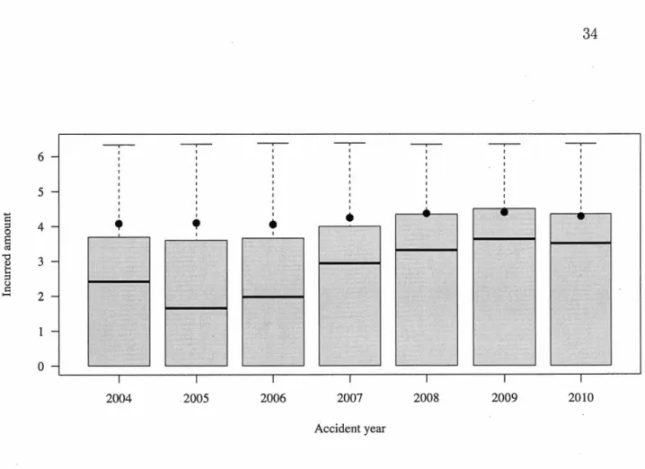
2016 is $16,067, and the incurred distribution for each occurrence year is presented in Figure 4.1.2. About 40% of the claüns close with a total paid amount of zero. If

32

we exdude daims with an incurred of zero as of December 3Pt 2016, the average incurred increases to $24,144.

The data is longitudinal, and each row of the database corresponds to a snapshot of a file. For each element in S, a snapshot is taken at the end of every quarter, and we have information fron1 the reporting date until December 31st 2016. Therefore, a daünant is represented by a maximu1n of 52 rows, since 52 is the number of quarters between January pt 2004 and December 3Pt 2016. A line is added in the database even if there is no new information, i.e., it could be possible that two consecutive lines provide precisely the same information. This method of storing daim data is not unique and varies from insurer to insurer. In Chapter 1, we have seen that intrinsically, the loss reserving problem is in continuous time. However, since we only have discrete information, we will now consider it a discrete problem, which means the constructed models will be discrete.

Example 4.1.1 All claimants with reporting date on the first quarter of year 2004 are represented by 52 rows, those with reporting date on the second quarter of year 2004 are represented by 51 rows, etc. Finally, all claimants with reporting date on the last quarter of year 2016 are represented by only one row.

The information vector for daim k at time

t

is given by

V~k)

=

(x~k),

c?)).

Therefore, information matrix about the whole portfolio at time t is given by

'D~s) = {V~k)}kES· Because the database contains a snapshot for each daimant at each quarter, it contains information 'Ds =

{'D~

5

)}{o.25t:

tEN,

t~52},

where t is

the number of years since T. Claimant features indu de characteristics of the

daimant himself, but also those regarding the daim and the policy associated with hin1. In order to validate the models, we need to know how n1uch has actually been paid for each daim. In portfolio

S

,

total paid amount

Cr

3 is still

33 0 0 0 0 on 0 0 0 en 0

a

'<::t .@ 0 (3 0 4-< 0 0 0 1-o M <1) J:J 0

a

0 ;:::l 0 z 0 N 0 0 0

s

0 1.01% 0.27% 0.05% 0.02% 0.00% 0.00% 2 3 4 5 6 7 8 9 Number of claimants

Figure 4.1.1: Number of claimants per claim.

open on December 3Pt 2016 (see Figure 4.1.3). In Figure 4.1.3, we can see that open daims are mostly from recent accident years. To overcome this issue, we use a subset S₇ = { k E S : T}k)

<

7} of S, i.e., we consider only accident years from 2004 to 2010 for both training and validation. This subset contains

36,843 daimants related to 30,483 daims. That way, only 0.67% of the daimants

are associated with daims that are still open as of the end of 2016, so we know the exact total paid amount for 99.33% of them, assuming no reopening after 2016.

For the small proportion of open daims, we assume that the incurred amount set by experts is the true total paid amount. Renee, the evaluation date is fixed to December 3Pt 2010 and we set t* = 7. This is the date at which the RBNS

reserve must be evaluated for daimants in S7 . This implies that the mo dels are

not allowed to use information past this date for their training. Infonnation after the evaluation date is only used for validation. A summary about sets S and S7

6 5 4 3 2 0 --.----1 1 1 1 1 2004 2005 --.----1 1 2006 --.----1 1 1 1 2007 Accident year --.----1 1 1 1 2008 --.----1 1 1 2009 34 2010

Figure 4.1.2: Distribution of final incurred by accident years {on a base 10 log

scale). The first quartile is equal to the minimum for all accident years since many claims close at zero. The average incurred for each accident year is represented

by a dot.

is clone in Table 4.1.1.

For simplicity and for computational purpose, the quarterly database is summa-rized to forma yearly database Vs7 =

{Vi

57

)}i!1,

where Vi57) = {Vik)}kES7· 70% of the 36,843 claimants have been sampled randomly to form the training set of in-dices

Tc S

7 , and the other 30% forms the validation set of indices

V

C

S

7 , which

gives the training and validation datasets Vr

=

{Vi

7

)}i!

1 and Vv

=

{Div)}i!

1 . A summary of training and validation datasets is clone in Table 4.1.2.

35

12 D Open

•

Settled ,-... rJ) "'0 10 s:: C<3 rJ) =' 0 -5 ₈

2

rJ)

s

₆ ·c; 0 4-o 0 ... ₄ Cl) .0

s

=' z ₂ 0 2004 2005 2006 2007 2008 2009 2010 2011 2012 2013 2014 2015 2016 Accident year

Figure 4.1.3: Status of claims on December 31st 2016.

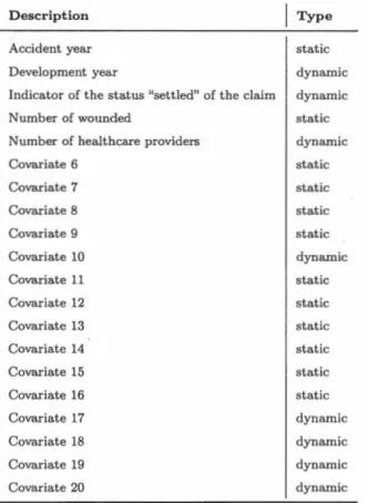
4.2 Covariates

In partnership with the insurance company, we have selected 20 covariates in order to predict total paid a1nount for each of the claimants, described in Table 4.2.1. Note that sorne variables have been censored due to the confidentiality agreement. To make models comparable, we use the same covariates for all of them. Sorne covariates are characteristics of the claimant and sorne are about the daim itself, as the accident year and the development year. Sorne of the covariates, such as the accident year, are static, which means their value do not change over time. These covariates are quite easy to handle because their final value is known since the reporting of the accident. However, sorne part of available information is expected to develop between t* and the closure date. More precisely, 8 of the 20 covariates are dynamic variables, as the number of healthcare providers. To handle those

36

Table 4.1.1: Comparison of complete set of claimants (S) and set of claimants

from accident years 2004-2010 (S7 ).

%

of open claims is on December 3Pt 2016.

Dataset

#

claims

#

clain1ants

%

of open claims

s

67,203 82,520 18.87

s1

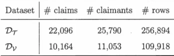
30,483 36,843 o.67

Table 4.1.2: Details about training and validation datasets.

Dataset

#

claims

#

claimants

#

rows

VT 22,096 25,790 256,894

Vv 10,164 11,053 109,918

dynamic covariates, we have, at least, the following two options:

• we can assume that they are static, which can lead to a bias in the predictions obtained, or;

• we can, for each of these variables,

(1)

adjust a dynamic model, (2) obtain a

prediction of the complete trajectory, and (3) use the algorithm conditionally to the realization of this trajectory. Moreover, it is possible that there is sorne dependence between these variables and therefore a n1ultivariate approach could be necessary.

In this work, we simply assume that values of dynamic covariates are frozen at

time t*. Also, notice th at the case reserve set by adj usters is not used as a

covariate. This information would probably be useful, but would make models non self-sufficient.

37

Table 4.2.1: Covariates used in the models.

Description Type

Accident year static

Development year dynamic

lndicator of the status "settled" of the claim dynamic

Number of wounded static

Number of healthcare providers dynamic

Covariate 6 static Covariate 7 static Covariate 8 static Covariate 9 static Covariate 10 dynamic Covariate 11 static Covariate 12 static Covariate 13 static Covariate 14 static Covariate 15 static Covariate 16 static Covariate 17 dynamic Covariate 18 dynamic Covariate 19 dynamic Covariate 20 dynamic

4.3 Training of XGBoost models

ln Section 3.3, we have seen that in order to fit an XGBoost model, we need the training response Cr3 for each daimant in the training set. However, 22% of the

daimants in S7 , mostly from recent accident years, are associated with daims that

are still not settled at t*

=

7, and their total paid amount Cr₃ is still unknown (see Figure 4,3.1). We therefore face a censored response variable issue. At this stage, several options are available:

1. The simplest solution is to train the 1nodel on a training set where only settled daims (or non censored dain1s) are induded. Renee, the response

Cil

a

·~ ü <...., 0 1-o ~ .D 8 ::s z

38

0 0 0 00 0 Open

•

Settled 0 0 0 \0 0 0 0 "<:t' 0 0 0 ('1 0 2004 2005 2006 2007 2008 2009 2010 Accident year

Figure 4.3.1: Status of claims on December 31st 201 O.

is known for all claimants. However, this leads to a selection bias because

claims that are already settled at t* tend to have shorter developments, and claims with shorter developments tend to have lower total paid amounts.

Consequently, the model is almost exclusively trained on simple claims with low training responses, and this leads to underestimation of the total paid amount for new daims. Furthern1ore, a significant proportion of the claimants are removed from the analysis, which causes a loss of information. We will further analyze this bias below.

2. In [LM16], a different and interesting approach is proposed: in order to cor-rect the selection bias induced by the presence of censored data, a strategy called "Inverse Probability of Censoring Weighting" (IPCW) is implemented, which involves assigning weights to observations to offset the lack of