Extension of Partitional Clustering Methods for Handling Mixed Data
Yosr Naija
LIP2, Faculty of Science of Tunis
Campus Universitaire
2092 El-Manar Tunis, Tunisia
[email protected]
Salem Chakhar
LAMSADE, University of Paris-Dauphine
Place du Mar´echal de Lattre de Tassigny
75775 Paris Cedex 16, Paris, France
[email protected]
and
´
Ecole Centrale Paris, Grande Voie des Vignes
92 295 Chˆatenay-Malabry Cedex, France
[email protected]
Kaouther Blibech
LIP2, Faculty of Science of Tunis
Campus Universitaire
2092 El-Manar Tunis, Tunisia
[email protected]
Riadh Robbana
LIP2, Faculty of Science of Tunis
Campus Universitaire
2092 El-Manar Tunis, Tunisia
[email protected]
Abstract
Clustering is an active research topic in data mining and different methods have been proposed in the literature. Most of these methods are based on the use of a distance measure defined either on numerical attributes or on categorical at-tributes. However, in fields such as road traffic and medi-cine, datasets are composed of numerical and categorical attributes. Recently, there have been several proposals to develop clustering methods that support mixed attributes. There are three basic categories of clustering methods: par-titional methods, hierarchical methods and density-based methods. This paper proposes an extension of partitional clustering methods devoted to mixed attributes. The pro-posed extension looks to create several partitions by us-ing numerical attributes-based clusterus-ing methods and then chooses the one that maximizes a measure—called “homo-geneity degree”—of these partitions according to categori-cal attributes.
1. Introduction
In applications such as telecommunications, road traffic, medicine and banking there is often a need to extract data measuring the evolution of some parameters that are useful for decision making. These parameters can be numerical (e.g. phone consumption, flow of cars, consumption of
to-bacco, balances of the customer) or categorical (e.g. day of the week, antecedents of a disease in a family, unemployed). Decision makers (e.g. traffic experts, doctors, or bank man-agers) have to understand and analyse these data to make decisions. For example, an expert of traffic should under-stand why there is a congestion in a period of day to avoid this situation, a doctor needs to know the reasons for which a group of people is ill to better dealt with the problem. They should find the factors that influence a given behavior. Clustering is a widely used technique in data mining ap-plications to achieve this goal. Generally, decision mak-ers have a limited information about datasets that they hold. Clustering allows to enrich these datasets and to identify similar or different behaviors between them. Concretely, it allows to partition a set of objects into classes based on defined criteria so that objects in the same class are more similar than objects within different classes [5, 9].
In the second half of 20th century, data mining commu-nity has proposed clustering methods that handle objects de-scribed only by numerical attributes such as K-means [12], or only by categorical ones such as K-mode [7]. However, as mentioned above, datasets in real-world applications are composed of both types of attributes. Since the late of 1990th, there have been several proposals to develop clus-tering methods that support mixed attributes (numerical and categorical ones). Most efforts have been oriented towards the extension of conventional clustering algorithms giving a new distance measure that handles mixed attributes. It
is important to note that both numerical and categorical at-tributes need to be considered during classification. How-ever, we think that numerical attributes are more discrim-inative than categorical ones since they explain better the differences that may exist between objects. Categorical at-tributes can be used latter to explain some behaviors. The use of weighted-sum like aggregation rules by combining both numerical and categorical attributes may be not suit-able since the definition of weights is not an obvious task.
In this paper, we present a clustering approach that deals with mixed attributes while giving more importance to nu-merical ones. There are three basic categories of clus-tering methods: partitional methods, hierarchical methods and density-based methods. The paper proposes an exten-sion to partitional clustering methods devoted to mixed at-tributes. The extension looks to create several partitions by using numerical attributes-based clustering methods and then chooses the one that maximizes a measure, that we called “homogeneity degree”, of these partitions according to categorical attributes.
This paper is organized as follows. Section 2 discusses some related work. Section 3 details the proposed approach. Section 4 presents an extended mixed-attributes partitional clustering algorithm. Section 5 presents some numerical results and discusses some important points. Section 6 con-cludes the paper.
2. Related work
2.1. Clustering and clustering approaches
Clustering allows to partition a set of objects into classes based on defined criteria so that objects in the same class are more similar than objects within different classes [5, 9]. More formally, given a set of n objects X =
{O1, O2, . . . , On}, clustering aims to find a function
f : X → {C1, C2, . . . , Ck}
that assigns each object Oi ∈ X to a class Cj (j =
1, · · · , k) (k represents the number of classes) .
Three main steps are important to cluster objects [9]: (i) feature selection where characteristics of objects (the at-tributes that describe objects) are identified; (ii) definition of a proximity measure which is often a distance function that will be used to measure similarity between objects. The choice of a given proximity measure depends largely on the application’s domain. An example of distance function is the Euclidean distance; and (iii) creation of classes where a clustering method is first identified and then used to create classes.
The basic categories of clustering methods are [5]:
• Partitional methods: these methods aim to decompose
objects into k classes. With this approach the num-ber of classes k is generally a predefined parameter. K-means [12], CLARANS [13] and K-mode [7] are examples of partitional clustering methods.
• Hierarchical methods: given n objects, this category
of methods aims to create different levels of partitions (from 1 to n − 1 levels). The levels are built either by merging at each step the two closest classes until ob-taining one class or by splitting, at each step, clusters that contain dispersed objects until obtaining n classes or satisfying a given criterion. Examples are: agglom-erative methods, divisive methods [10], BIRCH [15] and CURE [4] methods.
• Density-based methods: these methods group objects
into classes so that the surface or volume of these classes are dense “enough”. Density is computed us-ing pre-defined thresholds. DBSCAN [3] is one of the most used density-based methods. Squeezer [6] is a density-based method devoted to categorical attributes. There are other categories of clustering methods such as Grid-based methods but they are used only in specific do-mains like spatial data mining.
2.2. Mixed attributes-based clustering
There are three intuitive ideas to support mixed attributes clustering:
• The conversion of each categorical attribute into a
merical attribute. The clustering methods based on nu-merical attributes can then be used. However, it is diffi-cult sometimes to code a categorical attribute without understanding the meaning of this attribute [1]. For example, the conversion of an attribute color is more difficult than the conversion of an attribute month.
• The discretization of numerical attributes so that each
numerical attribute is converted into a categorical one by using a discretization method. Then the objects can be clustered by using one of the clustering methods based on categorical attributes. DSqueezer (Discretiz-ing before Us(Discretiz-ing Squeezer) [6] method follows this idea. The principal limit of this type of approach is the loss of information generated by discretizing.
• Conversion of the categorical attributes into binary
ones: each categorical attribute Aiwith d distinct val-ues is converted into d binary attributes where each at-tribute takes value 1 if the object is described by this attribute, 0 if not. In [14], Ralambondrainy follows this principle to create classes of objects with mixed
attributes. The disadvantage of this approach is that the conversion increases the number of attributes de-scribing the objects. Moreover, with this approach at-tributes are less meaningful after conversion [2]. More recently, more emphasized methods allowing to cluster objects described by mixed attributes have been pro-posed in the literature. These methods represent exten-sions of conventional methods (numerical attributes-based clustering methods or categorical attributes-based cluster-ing methods). Extensions consist in uscluster-ing a measure dis-tance that supports mixed attributes. The three cluster-ing steps mentioned earlier still apply with these extended methods.
K-prototype [8] is one of the first extended methods pro-posed in the literature. It is a combination of K-means [12] and K-mode [7] methods. The distance measure used with K-prototype is the sum of Euclidean distance, which is used to compute the distance between numerical attributes, and the simple matching measure used to dealt with categor-ical attributes where the distance between two objects is computed as the number of different attributes values be-tween these objects. To build classes, K-prototype follows the same steps as K-means and K-mode.
The authors of [2] propose a clustering method based on the algorithm of agglomerative hierarchical clustering methods and on a distance hierarchy that expresses similar-ity between attributes’ values. Every attribute is represented by a hierarchy. For categorical attributes this hierarchy is a tree where each node represents a possible value of the at-tribute and every link is valued by a weight representing the distance between these values. Concerning numerical attributes, the hierarchy is represented by only two nodes corresponding to the minimal and maximal values of the attribute. The distance between two objects is the total of distances between values of objects’ attributes based on the hierarchy distance. Given this distance measure, the [2]’s method begins by representing each class by one object and then an additional measure is used iteratively to merge the closest classes.
UsmSquezer (Squeezer for Unified Similarity Mea-sures) [6] is an extension of the categorical attribute-based Squeezer method. The authors propose a similarity mea-sure between an object O and a class C, which is the sum of similarity measure between categorical attributes and simi-larity measure between numerical attributes. The first one computed on basis of the proportion of objects of C having the same values as the studied object O. The second one is computed on the basis of the difference between values of each numerical attribute A of O and the mean value of the studied attribute for all objects of the class. The clustering algorithm of UsmSquezer remains the same as Squeezer.
There are several other methods supporting mixed at-tributes [1, 11]. Most of them rely on the definition of a
new distance measure that combines numerical and cate-gorical attributes. However and as mentioned previously in Section 1, we think that numerical attributes are more dis-criminative than categorical. The approach that we propose in the next section is an extension to partitional clustering methods.It looks to create several partitions by using numer-ical attribute-based clustering methods and then chooses the one that maximizes the “homogeneity degree” of these par-titions according to categorical attributes.
3. Proposed homogeneity degree-based
cluster-ing approach
The basic idea of the proposed approach is to apply a numerical attributes-based clustering method several times on the same datasets while changing some initial parame-ters such as the number of classes or the similarity thresh-olds. Then, for every obtained partition, a measure called homogeneity degree is computed. The homogeneity degree measures the homogeneity of a partition according to cate-gorical attributes. Finally, the partition that maximizes the homogeneity degree is selected. Algorithm 1 in Section 4 illustrates this idea. The objective of this section is to show how homogeneity degree is computed
The homogeneity degree of a partition depends on the homogeneity degrees of its classes and the homogeneity de-grees of attributes domains. Some useful definitions are in-troduced first.
3.1. Basic definitions
Definition 3.1 (Domain of categorical attribute). The
do-main of a categorical attribute Aiis denoted DOM (Ai) =
{ai1, ai2, . . . , ait} where aijis a possible value of Aiand t
is the number of possible values.
Definition 3.2 (Hierarchy of categorical attributes). A
hi-erarchy organizes attributes according to a “finer than” relationship, along with their level of details. Let A1and
A2be two categorical attributes. Then, A1 ⊆HA A2 sig-nifies that A1 is less general (or more finer) than A2. If there is not any hierarchical relation between A1 and A2,
A1and A2are said to be non hierarchical. This is denoted by A1 HAA2.
Example 1. Let month and trimester be two
categori-cal attributes. Let DOM (month) = {1, 2, . . . , 12} and
DOM (trimester) = {1, 2, 3, 4}. Then, month⊆HA
trimester.
Definition 3.3 (Labels of an object). A label is a set of
values of categorical attributes with no hierarchical rela-tionship among them. Let A1, A2, . . . , Anbe n categorical
A1, A2, . . . , An is defined as the Cartesian product of the
domains of A1, A2, . . . , An: DOM (A1) × DOM (A2) ×
· · ·×DOM (An). Accordingly, a label li∈ L is an instance
of DOM (A1) × DOM (A2) × · · · × DOM (An). The
no-tation Label(O) = li means that object O is described by
label li.
Example 2. Let A1, A2 and A3 be three categorical at-tributes associated respectively with the day number of the week (from 1 to 7), the type of day (Y if it is a holiday and N if not) and the month number (from 1 to 12). Figure 1 provides the set L of labels. The label l12(1 Y 12) for in-stance corresponds to a Monday of December, which is also a holiday.
Figure 1. Example of labels
3.2. Class homogeneity according to
cate-gorical attributes
Naturally, a class is homogeneous according to categori-cal attributes if its objects have the same label(s). However, a crisp definition of the notion of homogeneity may be very restrictive in practice and makes homogeneity largely de-pending on the application’s domain and on the datasets. The homogeneity degree concept as introduced in the rest of this section provides a fuzzy measure of homogeneity. Indeed, homogeneity degree takes its values in the range [0,1], where 1 indicates that the class is fully homogeneous and 0 indicates that the class is not homogeneous. A value between 0 and 1 represents the level to which a class is ho-mogeneous.
The definition of homogeneity degree requires the use of two thresholds α ∈ [0, 1] and β ∈ [0, 1] assuring the
co-herence of results. The practical utility of these parameters will be better explained in 5.3.1.
Next, some useful notations are introduced.
• X = {O1, O2, . . . , On}: a set of n objects.
• L = {l1, l2, . . . , lm}: a set of m labels (m ≤ n).
• Pk(C1, C2, . . . , Ck): a partition of k classes.
• SCij = {Or ∈ Ci : Label(Or) = lj}: the set of objects of class Cihaving the label lj.
• Sj = {Or∈ X : Label(Or) = lj}: the set of objects of X having the label lj.
• k · k: set cardinality symbol.
3.2.1
Membership degree of a label in
re-spect to a domain
The membership degree M Dα(lj, Ci) of a label lj in a class Ciin respect to a domain expresses the proportion of objects of Ci described by label lj in respect to the total number of objects of X having the label lj. M Dα(lj, Ci) is defined as follows: M Dα(lj, Ci) = ( kSCijk kSjk , if kSCijk kSjk ≥ α and k Sjk6= 0; 0, Otherwise (1)
As it is shown in Eq. 1, M Dα(lj, Ci) will be equal to 0 any time the proportion of objects described by label lj is strictly less than α. This ensures that Ci contains at least
α% of objects of X.
3.2.2
Homogeneity degree in respect to a
domain
The homogeneity degree of a class Ci in respect to a domain, denoted by HDα(Ci), is defined through Eq. 2:
HDα(Ci)= ½ 1 B· Pm j=1M Dα(lj, Ci), if B 6= 0; 0, Otherwise. (2) where B =k {lk : lk ∈ L ∧ M Dα(lk, Ci) > 0} k, that is, the number of labels lksuch that M Dα(lk, Ci) is strictly positive.
HDα(Ci) represents the average of labels’ membership degrees. Other formula such as the product of M Dα(lk, Ci)
(k = 1, · · · , m) or the maximum or minimum value of
3.2.3
Membership degree of a label in
re-spect to a class
The membership degree M Cα(lj, Ci) of a label ljin re-spect to a class Ci reflects the proportion of objects of Ci described by lj. In other words, M Cα(lj, Ci) permits to measure the importance of label lj to class Cj. Formally,
M Cα(lj, Ci) is computed as follows: M Cα(lj, Ci) = ( kSCijk kCik , if M Dα(lj, Ci) ≥ α; 0, Otherwise (3)
As it is shown in Eq. 3, only labels for which M Dα≥ α are included in the definition of M Cα(lj, Ci). This ensures that only the most important labels are considered in the computing of M Cα(lj, Ci).
3.2.4
Partial homogeneity degree of a
class
The partial homogeneity degree HCα(Ci) of class Ciis given by Eq. 4: HCα,β(Ci)= Pm j=1M Cα(lj, Ci), ifPmj=1M Cα(lj, Ci) ≥ β; 0, Otherwise (4)
The threshold β used in the definition of HCα(Ci) en-sures that only important labels are considered for comput-ing the partial homogeneity degree of the class.
3.2.5
Overall homogeneity degree of a
class
The overall homogeneity degree of a class Citakes into account the homogeneity degree of Ciin respect to the do-main and the partial homogeneity of Ci. It is denoted by
Dα,β(Ci) and computed through Eq. 5 hereafter:
Dα,β(Ci) = HDα(Ci) · HCα,β(Ci) (5) Intuitively, a class Ci is more homogeneous (resp. less homogeneous) than a class Cj if and only if Dα,β(Ci) >
Dα,β(Cj) (resp. Dα,β(Ci) < Dα,β(Cj)).
3.3. Partition homogeneity degree
accord-ing to categorical attributes
Let Pk(C1, C2, . . . , Ck) be a partition of k classes. The homogeneity degree DPα,β(Pk) of Pkis defined by the Eq. 6 below: DPα,β(Pk) = 1 k· k X i=1 Dα,β(Ci) (6)
It is important to note that other formula may also apply such as: DPα,β(P ) = i=kY i=1 Dα,β(Ci), DPα,β(P ) = min(Dα,β(Ci), · · · , Dα,β(Ck)), or DPα,β(P ) = max(Dα,β(Ci), · · · , Dα,β(Ck)). In the rest of this paper we suppose that Eq. 6 is used. The value of DPα,β(Pk) varies between 0 and 1. If
DPα,β(Pk)=1, the partition is said to be fully homoge-neous and if DPα,β(Pk)=0, then the partition is non ho-mogeneous. Otherwise, the partition Pk is homogenous to a level equal to DPα,β(Pk).
3.4. Illustrative example
Consider a set X of objects described by two attributes:
• Attribute A1 indicates if a day is a working day (be-tween Monday and Friday) or not: DOM (A1) =
{Y, N }.
• Attribute A2 indicates if a day is a holiday or not:
DOM (A2) = {Y, N }.
The L = {l1 = Y Y, l2 = Y N, l3 = N Y, l4 = N N } be the set of labels. Suppose that k S1 k= 5, k S2 k= 10,
k S3 k= 6, and k S4 k= 4. Let C1and C2be two classes defined on X. The content of these two classes is shown in Figure 2. Class C1 contains 13 objects (two are described by label l1, nine by l2and two by l4). Class C2contains 12 objects (three are described by label l1, one by l2, six by l3 and two by l4).
Consider now class C1 and suppose that α = 0.5 and
β = 0.1. Using Eq. 1 and Eq. 3, we get: • M D0.5(l1, C1) = 0; M C0.5(l1, C1) = 0,
• M D0.5(l2, C1) = 0.9; M C0.5(l2, C1) = 0.64,
• M D0.5(l3, C1) = 0; M C0.5(l3, C1) = 0,
Figure 2. ClassesC1andC2
For instance: M D0.5(l1, C1) = 0 (since||SC||S11,1|||| = 25 = 0.4 < α) and M D0.5(l4, C1) =||SC||S44,1|||| = 24 = 0.5.
Then, by using Eq. 2 and Eq. 4, we get:
• HD0.5(C1) = 12(M D0.5(l2, C1)+M D0.5(l4, C1)) = 0.7,
• HC0.5,0.1(C1) = M C0.5(l1, C1) + M C0.5(l2, C1) +
M C0.5(l3, C1) + M C0.5(l4, C1) = 0.86.
Next, the homogeneity degrees of classes C1and C2can be computed by Eq. 5. This leads to:
D0.5,0.1(C1) = HD0.5(C1) · HC0.5,0.1(C1) = 0.7 · 0.86
= 0.6
D0.5,0.1(C2) = HD0.5(C2) · HC0.5,0.1(C2) = 0.64
Finally, the homogeneity degree of partition P2(C1, C2) is computed by Eq. 6: DP0.5,0.1(P2) = 1 2(D0.5,0.1(C1) + D0.5,0.1(C2)) = 1 2(0.6 + 0.64) = 0.62
Tables 1, 2 and 3 hereafter give the values of Dα,β(C1),
Dα,β(C2) and DPα,β for some values of α and β. It is easy to see that for α = 0.1 and β = 0.5, class C1is more homogeneous than class C2, while for α = 0.5 and β = 0.1, C2is more homogeneous than C1.
α β HDα(C1) HCα,β(C1) Dα,β(C1) 0.1 1 0.6 0.1 0.5 0.6 1 0.6 0.9 1 0.6 0.1 0.86 0.6 0.5 0.5 0.7 0.86 0.6 0.9 0 0 0.1 0.64 0.58 0.9 0.5 0.9 0.64 0.58 0.9 0 0 0.1 0 0 1 0.5 0 0 0 0.9 0 0
Table 1. Values of HDα(C1), HCα(C1) and
Dα,β(C1) α β HDα(C2) HCα,β(C2) Dα,β(C2) 0.1 1 0.55 0.1 0.5 0.55 1 0.55 0.9 1 0.55 0.1 0.91 0.64 0.5 0.5 0.7 0.91 0.64 0.9 0.91 0.64 0.1 0.36 0.36 0.9 0.5 1 0 0 0.9 0 0 0.1 0.36 0.36 0.9 0.5 1 0 0 0.9 0 0
Table 2. Values of HDα(C2), HCα(C2) and
Dα,β(C2) α β Dα,β(C1) Dα,β(C2) DPα,β(P2) 0.1 0.6 0.55 0.58 0.1 0.5 0.6 0.55 0.58 0.9 0.6 0.55 0.58 0.1 0.6 0.64 0.62 0.5 0.5 0.6 0.64 0.62 0.9 0 0.64 0 0.1 0.58 0.36 0.47 0.9 0.5 0.58 0 0 0.9 0 0 0 0.1 0 0.36 0 1 0.5 0 0 0 0.9 0 0 0
Table 3. Values ofDPα,β(P2)for different
val-ues ofαandβ
3.5. Propositions
This section presents a series of propositions concerning the relationship between HDα, HCα,β, M Dαand M Cα. Proposition 1 (Relation between HDα and α). Giving a
class Ci,
• If maxjkSCkSjijkk) < α, then HDα(Ci) = 0 (part 1)
• If α = 1 and @ lj such that kSCkSjijkk = 1, then,
HDα(Ci) = 0 (sub-part 2.1). Otherwise HDα(Ci) =
• If there is at least one label ljsuch that kSCkSjijkk = 1,
then limα→1(HDα(Ci)) = 1 (part 3)
Proof (part 1). Given a class Ci, if for every label lj (j = 1, . . . , m), kSCijk
kSjk < α, then for every label lj (j = 1, . . . , m), M Dα(lj, Ci) = 0. Then, according to Eq. 2,
HDα(Ci) = 0.
Proof (part 2). The proof of the sub-part 2.1 is trivial
because this part is the consequence of part 1. For sub-part 2.2, given a class Ci, HDα(Ci) is equal to the mean of the M Dα(lj, Ci), ∀lj, that are different from 0. When
α = 1, we take into account only the values of kSCijk kSjk ,
∀lj, that are greater than 1 to compute HDα(Ci). Then, if there is at least one label lj such that kSCkSjijkk = 1, then
HDα(Ci) = 1
Proof (part 3). As mentioned above, HDα(Ci) is equal to the mean of the M Dα(lj, Ci) that are different from 0. If
α is close to 1, so for the computation of HDα(Ci), we take into account only the values of kSCijk
kSjk , ∀lj, that are greater than α. Then, the mean will be greater than α.
Proposition 2. Let P ljbe a set of r classes containing
ob-jects having the label lj. The following holds:
• Pri=1M Dα(lj, Ci) = 1 if ∀ Ci, M Dα(lj, Ci) 6= 0
(part 1)
• If for a given class Ci ∈ P Lj, M Dα(lj, Ci) > 0.5,
then ∀ Cm 6= Ci and ∈ P Lj, M Dα(lj, Cm) < 0.5
(part 2)
Proof (part 1). According to section 3.2.1,
M Dα(lj, Ci) is equal to the proportion of objects of a class Ci described by a label lj in respect to the total number of the objects of X having the label lj when this proportion is greater than α. Next, if ∀ Ci,
M Dα(lj, Ci) 6= 0, Then: r X i=1 M Dα(lj, Ci) = k SC1jk k Sjk +k SC2jk k Sjk + · · · +k SCrjk k Sjk = k SC1jk + k SC2jk + · · · + k SCrjk k Sjk = 1
Otherwise, we will have some proportions that will not be taken into account.
Proof (part 2). Trivial (consequence of part 1)
Proposition 3 (Relation between HCα,β(lj, Ci) and
M Dα(lj, Ci)). Let Ci be a class with labels list
Labels(Ci). If ∀lj ∈ Labels(Ci) M Dα(lj, Ci) ≥ α, then
HCα,β(Ci) = 1.
Proof. M Dα(lj, Ci) ≥ α means that M Cα(lj, Ci) = kSCijk
kCik . Consequently, if ∀lj ∈ Labels(Ci), then
M Dα(lj, Ci) ≥ α. Then, HCα,β(Ci) = k SCi1k k Cik +k SCi2k k Cik + · · · +k SCisk k Cik = k SCi1k + k SCi2k + · · · + k SCijk k Cik = 1
Proposition 4 (Relation between HCα,β and HDα). If
HDα(Ci) = 0, then HCα,β(Ci) = 0.
Proof. HDα(Ci) = 0 means that ∀lj, M Dα(lj, Ci) >
0. Thus, according to Eq. 3, M Cα(lj, Ci) = 0, ∀lj. Conse-quently, HDα,β(Ci) = 0.
4. Mixed-attributes clustering algorithm
Partitional clustering methods permit to obtain k classes of objects. The number of classes k is generally fixed be-fore running the algorithm. The idea of the proposed mixed-attributes clustering algorithm is to run several times one of the partitional clustering methods by varying the number of classes k from 2 to a maximal number of classes kmax cor-responding to the number of labels. At each iteration we compute the overall homogeneity degree DPα,β for differ-ent values of α and β. The values of α and β that maximize
DPα,βare stored. Then, the partition (and so the number of classes) that maximizes DPα,βis picked out.
Algorithm 1 that follows implements this idea. The pro-cedure PARTITIONING used in Algorithm 1 may ba any of the conventional partitional clustering methods that per-mits to obtain a partition of k classes based on numerical attributes.
Procedure Extended−Partitional−Clustering( X : Set of objects, L : Set of labels)
kmax← k L k
For k from 2 to kmax do Pk← PARTITIONING(k,X)
For α from 0 to 1 by stepα do For β from 0 to 1 by stepβ do
compute DPα,β(Pk)
end For end For
save (α, β, DPα,β(Pk)) for which
DPα,β(Pk) is maximal
end For
return the partition for which DPα,β(Pk) is maximal
End
Thresholds α and β vary from 0 to 1 by step stepα and stepβ, respectively. The parameters stepα and stepβ are chosen by the user before running the algorithm. Both
stepαand stepβmust be in the range ]0, 1[. Possible values are: 0.01, 0.1, and 0.2.
The complexity of the algorithm is O(kmax ·
(CP + 1
stepα 1
setpβ)) where CP is the complexity of PARTITIONINGalgorithm.
5. Experiment and discussion
This section presents an application of the proposed al-gorithm. The well-known K-means [12] partitional cluster-ing algorithm is used.
5.1. Datasets
The datasets is composed of 230 objects aleatory gener-ated. Each of these objects is described by 100 numerical attributes. Attributes values used are summed up as follows:
• E1 = {O1, O2, . . . , O50}: 50 objects where attributes values vary between 0 and 20.
• E2 = {O51, O52, . . . , O90}: 40 objects where at-tributes values vary between 150 and 170.
• E3 = {O91, O92, . . . , O130}: 40 objects where at-tributes values vary between 300 and 320.
• E4 = {O131, O132, . . . , O200}: 70 objects attributes values vary between 450 and 470.
• E5 = {O201, O202, . . . , O230}: 30 objects attributes values vary between 600 and 620.
For simplicity, the variation range for attributes values is the same for all attributes. This restriction has no conse-quence on the results.
A set of 10 labels L = {l1, l2, . . . , l10} is used. These labels are supposed to be created from categorical attributes. The distribution of labels in the different sets is given in Table 4.
Label Number of objects E1 E2 E3 E4 E5
l1 30 18 12 l2 5 5 l3 25 20 5 l4 15 14 1 l5 4 4 l6 21 21 l7 19 2 17 l8 51 6 4 41 l9 30 28 2 l10 30 30 Total 230 50 40 40 70 30
Table 4. Distribution of labels
5.2. Application of the algorithm
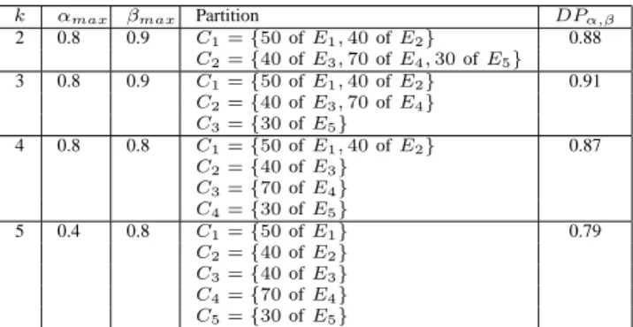
A summary of the results is given in Table 5. As it is shown in Table 5, the maximal value of overall homogeneity degree corresponds to partition k = 3 with α = 0.8 and
β = 0.9 (DP0.8,0.9(P3) = 0.91)
The justification of this result follows. First, note that for partition P3, objects of the sets E3 and E4 are in the same class, which is C2. Accordingly, all objects described by label l4are in class C2. This leads to M Dα(l4, C2) = 1. Moreover, class C2 contains the majority of objects described by label l8. For P4, in turn, the values of
M Dα(l4, C2) and M Dα(l4, C3) are less than 1; and the values of M Dα(l8, C2) and M Dα(l8, C3) will decrease. Consequently, DPα,β(P4) < DPα,β(P3). The same re-mark holds by comparing partition P3to partitions P2, and
P5.
k αmax βmax Partition DPα,β
2 0.8 0.9 C1= {50 of E1, 40 of E2} 0.88 C2= {40 of E3, 70 of E4, 30 of E5} 3 0.8 0.9 C1= {50 of E1, 40 of E2} 0.91 C2= {40 of E3, 70 of E4} C3= {30 of E5} 4 0.8 0.8 C1= {50 of E1, 40 of E2} 0.87 C2= {40 of E3} C3= {70 of E4} C4= {30 of E5} 5 0.4 0.8 C1= {50 of E1} 0.79 C2= {40 of E2} C3= {40 of E3} C4= {70 of E4} C5= {30 of E5}
Table 5. Results of the application of Algo-rithm 1
5.3. Discussion
This section first explains the role of the parameters α and β and their utility in explaining the behavior of datasets. A practical example illustrating this fact is then provided.
5.3.1
Role of
αand
βFirst, we note that to obtain coherent results, the values of α and β should be greater or equal to 0.5. This corre-sponds to the majority rule. Indeed, according to Proposi-tion 2, if α ≥ 0.5 and if M Dα(lj, Ci) > 0, then class Ci will contain more than 50% of objects having the label li. Moreover the fact that β have to be greater than 0.5 assures that the number of labels lj of which M Dα(lj, Ci) > 0 represents a proportion greater than 50% in the class. For instance, for partition P3in Table 5, we have:
• M D0.8(l1, C1) = 1,
• M D0.8(l3, C1) = 0.8,
• M D0.8(l5, C1) = 1,
• M D0.8(l9, C1) = 0.93 and
• HC0.8,0.9(C1) ≥ 0.9.
Then, class C1is described by labels l1, l3, l5and l9.
− For C2: • M D0.8(l2, C2) = 1, • M D0.8(l4, C2) = 1, • M D0.8(l6, C2) = 1, • M D0.8(l7, C2) = 0.89, • M D0.8(l8, C2) = 0.8 and • HC0.8,0.9(C2) ≥ 0.9.
Then, C2is described by labels l2, l4,l6, l7and l8.
− For C3:
• M D0.8(l10, C3) = 1, and
• HC0.8,0.9(C3) ≥ 0.9.
Then, C3is described by label l10.
This type of result can not be obtained with methods de-scribed in Section 2 since te use of a distance measure that handles mixed attributs does not grantee that the obtained classes are described by distinct labels.
Results such as ones presented above allow, in a second stage, to make decisions such as:
• Forecasting: the fact that each class is described with
distinct labels permits to conclude that each object having a label ljmust be included in a class for which label lj is representative. This permits to predict the behavior of any object.
• Detection of outlier: a new object Or described by a label lj is included in the nearest class Ciin terms of numerical attributes. If the label ljis not representative of class Ci, then object Oris an outlier.
5.3.2
Road traffic application
Consider that a road traffic datasets representing the number of vehicles passing in a point x of a road network each hour during one day. Each object is then described by 24 numerical attributes {A1, A2, . . . , A24}: A1is the num-ber of vehicles on 00h00, A2is the number of vehicles on 01h00, and so on. The objects are also described by 2 cat-egorical attributes A25and A26that represent respectively
working day and holiday with DOM (A25 = {Y, N } and
DOM (A26) = {Y, N }.
By applying one of numerical attributes-based clustering methods, the proposed approach assures that the objects in the same class are more similar than objects within different classes according to only numerical attributes. After that, the identification of the partition that maximizes the overall homogeneity degree permits to detect factors that influence the behaviors of datasets. For example, obtaining a class
C1 described by the label N N and N Y (α and β should be greater or equal to 0.5) indicates that the majority of the objects described by label N N or label N Y are in the same class. We can next conclude that the traffic during weekend is similar to the traffic during the holiday and that any new object whose values are recorded in a holiday or a weekend will have the same behavior as the representative labels of class C1. Moreover, we can detect the outliers as mentioned above and we can explain some facts like accidents or traffic lights problems.
6. Conclusion
In this paper, we first introduced the concept of homo-geneity degree. This concept permits to measure the level to which a class is homogenous in respect to categorical at-tributes. Then, we proposed an extended mixed-attributes clustering algorithm based on the notion of homogeneity degree. Currently, the extended algorithm requires the use of a conventional partitional clustering method. However, we intend to explore the possibility to extend the algorithm to apply with other type of clustering methods such as hier-archical or density-based ones.
References
[1] A. Ahmed and D. Lipika. A k-mean clustering algorithm for mixed numeric and categorical data. Data and Knowledge
Engineering, 63(2):503–527, 2007.
[2] H. Chung-Chian, C. Chin-Long, and S. Yu-Wei. Hierarchi-cal clustering of mixed data based on distance hierarchy.
In-formation Sciences, 177(20):4474–4492, 2007.
[3] M. Ester, H.-P. Kriegel, J. Sander, and X. Xu. A density-based algorithm for discovering clusters in large spatial data-bases with noise. In Proc. of 2nd Int. Conf. on Knowledge
Discovery and Data Mining (KDD), pages 226–231,
Port-land, Oregon, August 1996.
[4] S. Guha, R. Rastogi, and K. Shim. CURE: An efficient clustering algorithm for large databases. In Proc. of ACM
SIGMOD Int. Conf. on Management of Data, pages 73–84,
Seatle, USA, June 1998.
[5] M. Halkidi, Y. Batistakis, and M. Vazirgiannis. On cluster-ing validation techniques. Journal of Intelligent Information
[6] Z. He, X. Xu, and S. Deng. Scalable algorithms for clus-tering mixed type attributes in large datasets. International
Journal of Intelligent Systems, 20(10):1077–1089, 2005.
[7] Z. Huang. A fast clustering algorithm to cluster very large categorical data sets in data mining. In Research Issues on
Data Mining and Knowledge Discovery, 1997.
[8] Z. Huang. Extensions to the k-means algorithm for cluster-ing large data sets with categorical values. Data Mincluster-ing and
Knowledge Discovery, 2(3):283–304, 1998.
[9] A.-K. Jain, M. Murty, and P.-J. Flynn. Data clustering: A review. ACM Computing Surveys, 31(3):264–323, 1999. [10] L. Kaufman and P. Rousseeuw. Finding groups in data: An
introduction to cluster analysis. John Wiley & Sons, 1990.
[11] C. Li and G. Biswas. Unsupervised clustering with mixed numeric and nominal data—a new similarity based agglom-erative system. In Proc. of the First Asian Pacific Conference
on Knowledge Discovery from Databases, pages 35–61,
Sin-gapore, 1997.
[12] J. Mcqueen. some methods for classification and analy-sis of multivariate observations. In 5th Berkeley Symp. on
Math. Statistics and Probability, pages 281–298, Berkley,
CA: University of California Press, 1967.
[13] R.-T. Ng and J. Han. Efficient and effective clustering meth-ods for spatial data mining. In 20th Int. Conf. on Very Large
DataBases (VLDB), pages 144–155, Santiago, Chile,
Sep-tember 1994.
[14] H. Ralambondrainy. A conceptual version of the k-means algorithm. Pattern Recognition Letters, 16(11):1147–1157, 1995.
[15] T. Zhang, R. Ramakrishnan, and M. Livny. BIRCH: An ef-ficient data clustering method for very large databases. In
Proc. of ACM SIGMOD Int. Conf. on Management of data,