HAL Id: pastel-00006196
https://pastel.archives-ouvertes.fr/pastel-00006196
Submitted on 30 Jun 2010
HAL is a multi-disciplinary open access
archive for the deposit and dissemination of
sci-entific research documents, whether they are
pub-lished or not. The documents may come from
teaching and research institutions in France or
abroad, or from public or private research centers.
L’archive ouverte pluridisciplinaire HAL, est
destinée au dépôt et à la diffusion de documents
scientifiques de niveau recherche, publiés ou non,
émanant des établissements d’enseignement et de
recherche français ou étrangers, des laboratoires
publics ou privés.
logic
Olivier Delande
To cite this version:
Olivier Delande. Symmetric dialogue games in the proof theory of linear logic. Computer Science [cs].
Ecole Polytechnique X, 2009. English. �pastel-00006196�
Th`ese de Doctorat Sp´ecialit´e Informatique
Symmetric dialogue games in the proof theory of
linear logic
Pr´esent´ee et soutenue publiquement par
Olivier Delande
le 15 octobre 2009
devant le jury compos´e de
Claudia Faggian
Andr´e Hirschowitz Rapporteur
Olivier Laurent
Paul-Andr´e Melli`es
Dale Miller Directeur de th`ese
Acknowledgements
My first and foremost thanks go to my adviser Dale Miller for his support over the past three years. He not only provided highly valuable advice for the technical aspects of my research, but also the scientific vision that helped me put that work into perspective. On an equally important topic, he was always available and encouraging, and brought me confidence when I needed it. He also taught the first course I ever attended on the topic of logic, so I owe him my taste for this domain.
I am grateful to Andr´e Hirschowitz and Laurent Regnier for their extensive work in reviewing my thesis. Many of the ideas developed in this thesis were inspired by the discussions I had with Claudia Faggian and Paul-Andr´e Melli`es, so I would like to thank them for that. I am honoured that both of them, together with Olivier Laurent, accepted to be part of my jury.
I would like to thank Martin Hyland for welcoming me as a research visitor at the DPMMS in Cambridge, where I designed the concurrent game model described in Chapter 4 of this document. I had the privilege to work at the LIX, and I would like to thank my colleagues for making it a wonderful work environment, starting with the extremely helpful administrative staff, Catherine, Isabelle, James, Lydie, Marie-Jeanne and Matthieu, my other colleagues from the Tarski⊥`Church office, Alexis, David, and Vivek, later joined by Alexandre and Ivan. Special thanks go to Alexis whose work was inspirational and who provided useful advice. I also thank my other colleagues at Parsifal, the LIX and beyond, Anne-Laure, Andrew, Bruno, Carlos, Catuscia, David, Denis, Elaine, Florian, Fran¸cois, Frank, Jesus, Jo¨elle, Kaustuv, Laurent, Lutz, Matteo, Miki, Nicolas, Romain, Samuel, Stefan, St´ephane, Sylvain, Ulrich, Zach, . . . This list is by no means complete.
Last but not least, thanks to my family and friends for being supportive and to Florence who shared the whole adventure with me.
Contents
Introduction 1
1 Preliminaries 3
1.1 First-order classical logic . . . 3
1.2 Sequent calculus . . . 4
1.3 Linear logic . . . 7
1.4 Focalisation . . . 9
1.5 Multifocalisation . . . 12
1.6 Proof theory and computation . . . 13
1.7 Games and logic . . . 14
1.8 The neutral approach . . . 15
2 Additive neutral games 17 2.1 An additive neutral game . . . 17
2.1.1 Hintikka’s additive game for truth . . . 17
2.1.2 A neutral presentation . . . 20
2.1.3 Computation as dual proof search . . . 23
2.1.4 Interaction as proof normalisation . . . 24
2.2 Simple games for a fragment of MALL . . . 25
3 A sequential neutral game for MALL 29 3.1 Unrestricted multiplicatives . . . 29
3.1.1 Incompleteness . . . 29
3.1.2 Concurrency and focusing . . . 30
3.2 Proof system . . . 31 3.3 Basic definitions . . . 32 3.4 Neutral expressions . . . 32 3.5 Neutral graphs . . . 32 3.5.1 Interacting multiplicatives . . . 34 3.5.2 A neutral presentation . . . 37
3.6 Positions and moves . . . 39
3.6.1 Positions . . . 39 3.6.2 Micro-moves . . . 41 3.6.3 Macro-moves . . . 45 3.7 Examples . . . 45 3.7.1 Indeterminacy . . . 46 3.7.2 Atoms . . . 47
3.8 Winning strategies and cut-free proofs . . . 48
4 A concurrent neutral game for MALL 55 4.1 Introduction . . . 55
4.1.1 Non-uniformity . . . 55
4.1.2 Locality and concurrency . . . 56
4.1.3 The [⊤] rule . . . 56
4.1.4 Failure . . . 57
4.2 Proof system . . . 58
4.3 Neutral graphs . . . 59
4.4 Subgraphs . . . 60
4.5 Micro-moves . . . 63
4.6 Macro-moves and positions . . . 66
4.6.1 Definition . . . 66
4.6.2 Macro-moves as phases . . . 67
4.7 Strategies . . . 71
4.8 Winning strategies and proofs . . . 73
4.8.1 Strategy classes . . . 73
4.8.2 Goal trees . . . 73
5 Extensions 75 5.1 Explicit cuts . . . 75
5.1.1 Infinite interactions . . . 76
5.1.2 An alternate cut micro-move . . . 78
5.1.3 Winning strategies and proofs . . . 80
5.2 Exponentials . . . 81
5.3 First-order quantification . . . 82
5.4 Equality . . . 84
5.5 Fixed points . . . 85
6 Related and future work 87
Introduction
There is no absolute, unique notion of truth. In mathematics, we usually think of a true statement as one that can be proved. The late 19th century and the 20th century saw considerable efforts to formalise mathematics, in an attempt to set the bases of sound reasoning that everyone would agree on. As a byproduct of this effort, the development of proof theory provides formal ways to rep-resent mathematical proofs, but also gives the ability to reason about proofs themselves. A proof is a comprehensive collection of arguments establishing the truth of a statement. It is a self-contained object, that can be written once and for all.
However, proofs are not the only way to convince someone of the truth of a statement. Consider two persons called the Player and the Opponent. If the Player wants to convince the Opponent of the truth of a statement, she might opt for an interactive approach by letting the Opponent ask questions and delivering her arguments as needed. Debating is an example of such an interaction, and varies in its rules and degrees of formality. Logicians incorporate elements of game theory to study interaction. In the context of computer science, this line of research provides models of the interaction between a program and the environment it is running in.
Determining the relationship between the static notion of truth defined by proofs, and the dynamic one defined by interaction, is a vast field of research. Paul Lorenzen, who developed dialogue games, even considered games as prim-itive objects serving as a foundation for logic. A session of interaction, or play in the game-theoretic terminology, will typically involve only some of the argu-ments that can be found in a proof, much like in an examination: the examiner— the Opponent—tests the examinee—the Player—’s knowledge by asking some questions and verifying the answers given by the examinee, but she is not likely to test the whole subject in a single session. The important point is that the examiner has the power to ask any question pertaining to the subject. The only way for the examinee to be absolutely sure to pass the test is to know the whole subject. In the same fashion, a proof can be seen as a winning strategy allowing the Player to succeed in every play.
This fundamental asymmetry between the examinee and the examiner, or the Player and the Opponent, is pervasive in mainstream game semantics for logic. If a statement is provable, then the Player is able to defend it against all possible attacks by the Opponent. Conversely, if a statement is not provable, then the Opponent is able to defeat the Player by asking the right questions. In the former case, the Player’s winning strategy can be seen as a proof. In the latter case, nothing much is done with the Opponent’s winning strategy, which is merely seen as a refutation of the Player’s arguments. An interesting question is whether the Opponent’s strategy can be seen as a proof of the negation of the Player’s statement. In this thesis, we develop an original neutral approach to proof search. In our games, the two players have symmetric roles. Instead of being an examiner and an examinee, they are two parties attempting to prove opposite statements. The winning strategies of either player are seen as proofs of the statement she defends.
Our work is part of the computation-as-proof-search tradition. Instead of
considering proofs as preexisting objects that can be seen as winning strategies in the interaction, we see each step of the interaction as a step in two simultaneous exhaustive searches for the proofs of two dual formulae. We will work in the multiplicative and additive fragment of linear logic (MALL), which has two important advantages. Firstly, it is symmetric enough to allow a single process to perform two orthogonal proof searches. Secondly, it is not complete, i.e. the fact that a formula is not provable does not imply that its negation is. In other words, refuting a statement is necessarily different from proving its negation, highlighting the relevance of our approach. The formalism of choice for representing proofs will be sequent calculus, as it is the perfect basis for proof search and enjoys the symmetries we require. Moreover, the property of focalisation of linear logic will be thoroughly used in this thesis, and we will demonstrate its significance in interaction.
Outline of the thesis
• Chapter 1 introduces the fundamental notions used in our work. In par-ticular, the reader will find a presentation of sequent calculus, linear logic, and focalisation. We also present briefly the scope of the neutral approach and put it into the perspective of the history of logic and games.
• Chapter 2 develops the neutral approach in the restricted additive setting for which it was first designed by Miller and Saurin [MS06]. The focus is put on the particularities of dual proof search and the properties that will be preserved in the games for MALL.
• Chapter 3 describes a neutral game for MALL which is sequential in na-ture. The game-theoretic model is simple and the main result establishes the equivalence, for each player, between the provability of the player’s statement and the existence of a winning strategy. Some of this material was covered in our publications [DM08, DMS09].
• Chapter 4 introduces a new game model allowing for enough concurrency to establish a correspondence between proofs and winning strategies. • Chapter 5 investigates a few extensions of our game model. In particular,
we discuss the introduction of explicit cut moves in the game.
• Chapters 6 and 7 discuss related and future work and summarise the contributions of the thesis.
Preliminaries
This chapter presents core concepts that will be used throughout this thesis. We introduce linear logic through its sequent calculus, obtained by restricting the structural rules of the sequent calculus LK for classical logic. We also discuss focalisation, perhaps the most outstanding result on linear logic, and one of its extensions, multifocalisation. We finally introduce dialogue games for logic and our neutral approach.
1.1
First-order classical logic
Logic manipulates formulae which are mathematical statements written in a formal language. The features of a specific language determine the expressive-ness of the logic. The more constructions the language allows, the richer the logic will be. Propositional languages allow logics to describe finite behaviour. Expressing finite statements about infinitely many objects requires at least a first-order language. With such a language, it is possible to quantify over the elements of a set, as in “there exists an element of the set such that . . . ” or “for all elements of the set, . . . ”, which is familiar to any mathematician. Other, higher-order settings exist, in which it is possible to quantify over more complex objects such as relations.
A first-order language consists of
• a countable set of function symbols, each one being associated with a natural number called its arity,
• a countable set of variables,
• a countable set of predicate symbols, each one being associated with a natural number called its arity.
Function symbols with arity 0 are also referred to as constant symbols. We will now assume that a first-order language is fixed. Terms are inductively defined as follows. A variable is a term. If f is a function symbol with arity n, and t1, . . . , tn are terms, then f (t1, . . . , tn) is a term.
We can now define formulae. Formulae of first-order classical logic are in-ductively defined by the following grammar.
F, F′::= P (~t) | F ∨ F′ | ⊥ | F ∧ F′| ⊤ | F → F′ | ∀xF | ∃xF | ¬F where P is a predicate symbol of arity n, ~t = t1, . . . , tn is a list of n terms, and
x is a variable. A formula of the form P (~t) is an atom. ∨, ⊥, ∧, ⊤, →, ∀, ∃, and ¬ respectively represent disjunction, falsehood, conjunction, truth, implication, universal quantification, existential quantification, and negation. F ≡ G is an abbreviation for (F → G) ∧ (G → F ).
1.2
Sequent calculus
Proof theory is the formal study of mathematical proofs. There are many ways to represent proofs formally, and the one we are particularly interested in is sequent calculus. Sequent calculus was introduced by Gentzen [Gen69] as a proof system for classical logic named LK, and has been adapted to other logics since then. One of the strengths of this formalism is its symmetry.
A sequent is an expression of the form x1, . . . , xm; F1, . . . , Fn⊢ G1, . . . , Gp,
where x1, . . . , xmis a list of distinct variables called the signature and F1, . . . , Fn
and G1, . . . , Gp are formulae. The sequent x1, . . . , xm; F1, . . . , Fn⊢ G1, . . . , Gp
is a formal way of expressing the statement ∀x1. . . ∀xm F1∧ . . . ∧ Fn → G1∨
. . . ∨ Gp, i.e. that the disjunction of the Gi holds under the assumption of the
conjunction of the Fi. In sequent calculus, reasoning is expressed by inference
rules of the form
P1 . . . Pn
C
where P1, . . . , Pnare sequents called the premises of the rule and C is a sequent
called the conclusion of the rule. An inference rule formalises a step of reasoning in a proof, expressing that the conclusion follows from the premises. Figure 1.1 gives the rules of LK. Σ stands for a list of variables, Γ and ∆ for lists of formulae, x for a variable, and F , F1and F2 for formulae. Notice that the signature of a
sequent is almost never modified by a rule. As a result it is usually omitted. A proof is built by combining inference rules in a tree structure. For example, we can formally prove in LK the syllogism “all humans are mortal; Socrates is human; therefore Socrates is mortal”. We encode this syllogism as the formula (∀x (H(x) → M (x))) ∧ H(s) → M (s). The proof is H(s) ⊢ H(s) init M (s) ⊢ M (s) init H(s) → M (s), H(s) ⊢ M (s) →L ∀x (H(x) → M (x)), H(s) ⊢ M (s) ∀L ∀x (H(x) → M (x)), (∀x (H(x) → M (x))) ∧ H(s) ⊢ M (s) ∧L2 (∀x (H(x) → M (x))) ∧ H(s), (∀x (H(x) → M (x))) ∧ H(s) ⊢ M (s) ∧L1 (∀x (H(x) → M (x))) ∧ H(s) ⊢ M (s) CL ⊢ (∀x (H(x) → M (x))) ∧ H(s) → M (s) →R in which we omitted the XL and XR rules for the sake of brevity.
The sequent at the bottom of a proof is called its conclusion. The notion of derivation generalises the notion of proof. In a proof, all the sequents at the leaves of the tree are the conclusions of rules with no premises. In a derivation, such a leaf is said to be closed. An open leaf is simply a sequent which is not the conclusion of any rule. The collection of all the open leaves is called the frontier of the derivation. A derivation thus expresses that its conclusion follows from its frontier.
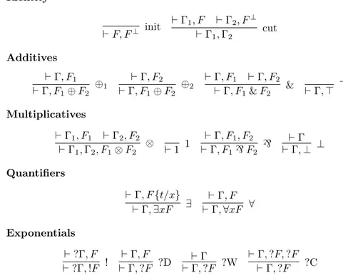
Inference rules are classified into groups. The identity group consists of the rules that identify two formulae: the init and cut rules. The init rule expresses a fundamental axiom of logic: a formula implies itself. The cut rule allows to introduce lemmas in a proof. It combines two proofs, one of them having the lemma as a conclusion, the other one having the lemma as a hypothesis. The logical rules express the logical meaning of the connectives. Each logical
Identity Σ; F ⊢ F init Σ; Γ1⊢ ∆1, F Σ; Γ2, F ⊢ ∆2 Σ; Γ1, Γ2⊢ ∆1, ∆2 cut Logical rules Σ; Γ, F1⊢ ∆ Σ; Γ, F2⊢ ∆ Σ; Γ, F1∨ F2⊢ ∆ ∨L Σ; Γ ⊢ ∆, F1 Σ; Γ ⊢ ∆, F1∨ F2 ∨R1 Σ; Γ ⊢ ∆, F2 Σ; Γ ⊢ ∆, F1∨ F2 ∨R2 Σ; Γ ⊢ ∆ Σ; Γ, ⊤ ⊢ ∆ ⊤L Σ; Γ ⊢ ∆, ⊤ ⊤R Σ; Γ, F1⊢ ∆ Σ; Γ, F1∧ F2⊢ ∆ ∧L1 Σ; Γ, F2⊢ ∆ Σ; Γ, F1∧ F2⊢ ∆ ∧L2 Σ; Γ ⊢ ∆, F1 Σ; Γ ⊢ ∆, F2 Σ; Γ ⊢ ∆, F1∧ F2 ∧R Σ; Γ, ⊥ ⊢ ∆ ⊥L Σ; Γ ⊢ ∆ Σ; Γ ⊢ ∆, ⊥ ⊥R Σ; Γ1⊢ ∆1, F1 Σ; Γ2, F2⊢ ∆2 Σ; Γ1, Γ2, F1→ F2⊢ ∆1, ∆2 →L Σ; Γ, F1⊢ ∆, F2 Σ; Γ ⊢ ∆, F1→ F2 →R Σ, x; Γ, F ⊢ ∆ Σ; Γ, ∃xF ⊢ ∆ ∃L Σ; Γ ⊢ ∆, F {t/x} Σ; Γ ⊢ ∆, ∃xF ∃R Σ; Γ, F {t/x} ⊢ ∆ Σ; Γ, ∀xF ⊢ ∆ ∀L Σ, x; Γ ⊢ ∆, F Σ; Γ ⊢ ∆, ∀xF ∀R Σ; Γ ⊢ ∆, F Σ; Γ, ¬F ⊢ ∆ ¬L Σ; Γ, F ⊢ ∆ Σ; Γ ⊢ ∆, ¬F ¬R Structural rules Σ; Γ ⊢ ∆ Σ; Γ, F ⊢ ∆ WL Σ; Γ ⊢ ∆ Σ; Γ ⊢ ∆, F WR Σ; Γ, F, F ⊢ ∆ Σ; Γ, F ⊢ ∆ CL Σ; Γ ⊢ ∆, F, F Σ; Γ ⊢ ∆, F CR Σ; Γ1, F2, F1, Γ2⊢ ∆ Σ; Γ1, F1, F2, Γ2⊢ ∆ XL Σ; Γ ⊢ ∆1, F2, F1, ∆2 Σ; Γ ⊢ ∆1, F1, F2, ∆2 XR
In the ∀L and ∃R rules, t is a term containing variables from Σ only. In the ∃L and ∀R rules, x is not free in the conclusion.
rule deals with the main connective of a specific formula, called the principal formula, leaving the other formulae of the sequent, which form the context, unchanged. Each inference rule is named after that connective. The suffixes “L” and “R” after the name of an inference rule mean that the principal formula is respectively on the left and on the right of the ⊢ symbol. The structural rules have no logical content, but express properties of the sequents themselves. In particular, they imply that in a sequent Γ ⊢ ∆, the order and multiplicities of the formulae in Γ and ∆ do not matter. In other words that Γ and ∆ could be seen as sets.
LK is highly symmetric. For each one of the pairs of connectives ∨/∧, ⊥/⊤, and ∃/∀, the right rule of a connective behaves like the left rule of the other. This is the well-known De Morgan duality. The following equivalences are provable.
¬(F1∨ F2) ≡ ¬F1∧ ¬F2 ¬(F1∧ F2) ≡ ¬F1∨ ¬F2
¬⊥ ≡ ⊤ ¬⊤ ≡ ⊥
¬∃xF ≡ ∀x¬F ¬∀xF ≡ ∃x¬F
F1→ F2≡ ¬F1∨ F2 ¬¬F ≡ F
It is therefore possible to put formulae in negation normal form where negation is applied to atoms only, and where there is no implication. An atom or the negation of an atom is called a literal.
The fundamental property of LK is cut admissibility. An inference rule is admissible when removing this rule from the proof system does not change the set of provable sequents.
Theorem 1.2.1 (Cut admissibility). The cut rule of LK is admissible. Although Gentzen originally stated this result in this way, he proved a stronger result: every LK proof can be effectively transformed into a cut-free proof. This procedure pushes cuts higher in a proof. For example pushing a cut through a disjunction is done as follows:
π3 Γ1⊢ ∆1, Fi Γ1⊢ ∆1, F1∨ F2 ∨Ri π1 Γ2, F1⊢ ∆2 π2 Γ2, F2⊢ ∆2 Γ2, F1∨ F2⊢ ∆2 ∨L Γ1, Γ2⊢ ∆1, ∆2 cut π3 Γ1⊢ ∆1, Fi πi Γ2, Fi⊢ ∆2 Γ1, Γ2⊢ ∆1, ∆2 cut
The cut elimination procedure gives a computational interpretation of se-quent calculus. In particular, the Curry-Howard isomorphism sees proofs as programs, and cut elimination corresponds to program execution.
An immediate corollary is the consistency of the logic. A logic is inconsis-tent when two dual formulae F and ¬F are provable. If classical logic were inconsistent, then the empty sequent would be provable by the cut rule
⊢ F ⊢ ¬F
⊢ cut
and, by the admissibility of cut, there would be a cut-free proof of the empty sequent. A case analysis shows that there is no cut-free proof of any sequent of the form ⊢ ⊥, . . . , ⊥.
Cut admissibility makes cut-free proofs objects worthy of consideration. Provability is preserved when eliminating cut. Cut-free derivations have a useful property.
Proposition 1.2.2. In a cut-free derivation, every formula is a subformula of a formula occurring in the conclusion.
Here, F is a subformula of G if it is a subtree of an instance Gσ of G. This result holds because the cut rule is the only one to introduce brand new formulae (reading derivations bottom-up). With this result we recast cut-free sequent calculus by replacing the notion of formula with the notion of formula occurrence, which is formally a location in the syntactic tree of a formula. For example, the formula F ∨ F has two distinct occurrences of the subformula F .
Another useful property of LK is that the init rule can be restricted to atoms. Proposition 1.2.3. Restricting the init rule to the atomic case does not affect provability.
Later on, we will consider a logic without atoms. The init rule will then be admissible.
1.3
Linear logic
Linear logic was introduced by Girard [Gir87]. It emerged from a semantic study of polymorphic λ-calculus. We choose a syntactic approach by introducing it through its sequent calculus LL, obtained by restricting the structural rules of LK.
The weakening (WL and WR) and contraction (CL and CR) rules of LK express that one can always weaken a statement by requiring an additional hypothesis or allowing an additional conclusion, and that multiple occurrences of a formula are as good as one. In a sequent Γ ⊢ ∆, the lists Γ and ∆ can be considered as sets. Linear logic is obtained by removing the weakening and contraction rules. In our presentation we also internalise the XL and XR rules. In other words, Γ and ∆ are now multisets of formulae.
One of the interesting consequences is that previously interchangeable sets of inference rules for the logical connectives are not equivalent any more. For example we chose the following right rules for disjunction in LK:
Γ ⊢ ∆, F1
Γ ⊢ ∆, F1∨ F2 ∨R1
Γ ⊢ ∆, F2
Γ ⊢ ∆, F1∨ F2 ∨R2
but we could have chosen the following rule instead: Γ ⊢ ∆, F1, F2
Γ ⊢ ∆, F1∨ F2 ∨R
Those two presentations can be proved equivalent only with the structural rules. Therefore we obtain two distinct disjunctions in linear logic, respectively de-noted to by ⊕ and`. Similarly, we get two conjunctions & and ⊗:
Γ ⊢ ∆, F1 Γ ⊢ ∆, F2
Γ ⊢ ∆, F1& F2 &
Γ1⊢ ∆1, F1 Γ2⊢ ∆2, F2
The same goes for the units ⊥ and ⊤, which become four units: 0 for ⊕, ⊥ for `, ⊤ for &, and 1 for ⊗. In that context, the De Morgan dual pairs are ⊕/&, 0/⊤, ⊗/`, and 1/⊥. ⊕, &, 0, and ⊤ make up the additive fragment of linear logic (ALL). ⊗,`, 1, and ⊥ make up the multiplicative fragment of linear logic (MLL). All eight of them make up the multiplicative and additive fragment of linear logic (MALL).
We will mostly be interested in MALL, which has a highly symmetric sequent calculus well suited to our approach. Its provability is decidable, more precisely PSPACE-complete [LMSS92, Kan94]. However, we present the full first-order linear logic here. The formulae of first-order linear logic are inductively defined by the following grammar.
F, F′ ::= P (~t) | P (~t)⊥| F ⊕ F′| 0 | F & F′| ⊤ | F ⊗ F′
| 1 | F ` F′ | ⊥
| !F | ?F | ∀xF | ∃xF
where P is a predicate symbol of arity n, ~t = t1, . . . , tn is a list of n terms, and
x is a variable. A formula of the form P (~t) is an atom.
In addition to the MALL connectives and first-order quantifiers, linear logic contains two connectives ! and ? called exponentials. Girard included them to recover the weakening and contraction rules in a controlled way. This allows intuitionistic logic to be encoded into linear logic, for example.
We did not include negation and implication as actual connectives. Like in LK, the ability to put formulae in negation normal form makes them superfluous. In the grammar, P (~t)⊥is a negated atom. Negation is an involution, inductively defined as (F1⊕ F2)⊥= F1⊥& F2⊥ (F1& F2)⊥= F1⊥⊕ F2⊥ 0⊥= ⊤ ⊤⊥= 0 (F1⊗ F2)⊥= F1⊥` F2⊥ (F1` F2)⊥= F1⊥⊗ F2⊥ 1⊥= ⊥ ⊥⊥= 1 (!F )⊥= ?F⊥ (?F )⊥= !F⊥ (∃xF )⊥= ∀xF⊥ (∀xF )⊥= ∃xF⊥
Linear implication F1⊸F2is defined as F1⊥` F2.
The sequent calculus for linear logic, LL, is presented in Figure 1.2. Due to the perfect symmetry of left and right rules, we opted for the mono-sided presentation, i.e. with sequents of the form ⊢ Γ. A sequent Γ ⊢ ∆ is replaced with ⊢ Γ⊥, ∆.
Many properties of LK are preserved in LL, including Theorem 1.2.1 and Propositions 1.2.2 and 1.2.3. The cut elimination step for additives is of partic-ular interest. When pushing a cut through a pair of dual formulae F1&F2/F1⊥⊕
F⊥ 2 π1 ⊢ Γ1, F1 π2 ⊢ Γ1, F2 ⊢ Γ1, F1& F2 & π3 ⊢ Γ2, Fi⊥ ⊢ Γ2, F1⊥⊕ F2⊥ ⊕i ⊢ Γ1, Γ2 cut πi ⊢ Γ1, Fi π3 ⊢ Γ2, Fi⊥ ⊢ Γ1, Γ2 cut
only one of π1 and π2 is kept. In the context of such an interaction between
Identity ⊢ F, F⊥ init ⊢ Γ1, F ⊢ Γ2, F⊥ ⊢ Γ1, Γ2 cut Additives ⊢ Γ, F1 ⊢ Γ, F1⊕ F2 ⊕1 ⊢ Γ, F2 ⊢ Γ, F1⊕ F2 ⊕2 ⊢ Γ, F1 ⊢ Γ, F2 ⊢ Γ, F1& F2 & ⊢ Γ, ⊤ ⊤ Multiplicatives ⊢ Γ1, F1 ⊢ Γ2, F2 ⊢ Γ1, Γ2, F1⊗ F2 ⊗ ⊢ 1 1 ⊢ Γ, F1, F2 ⊢ Γ, F1` F2 ` ⊢ Γ ⊢ Γ, ⊥ ⊥ Quantifiers ⊢ Γ, F {t/x} ⊢ Γ, ∃xF ∃ ⊢ Γ, F ⊢ Γ, ∀xF ∀ Exponentials ⊢ ?Γ, F ⊢ ?Γ, !F ! ⊢ Γ, F ⊢ Γ, ?F ?D ⊢ Γ ⊢ Γ, ?F ?W ⊢ Γ, ?F, ?F ⊢ Γ, ?F ?C
Figure 1.2: Mono-sided sequent calculus for linear logic.
& rule in a derivation. Such an operation is called slicing a derivation, and the resulting object is an (additive) slice. We will use the following notation for instances of the & rule where a slice is taken:
⊢ Γ, F1
⊢ Γ, F1& F2 &1
⊢ Γ, F2
⊢ Γ, F1& F2 &2
1.4
Focalisation
Andreoli [And92] proved a fundamental result about linear logic. With efficient logic programming in mind, Andreoli developed deep insights into the structure of the cut-free proofs in LL in an effort to reduce non-determinism in proof search.
For some inference rules it is the case that the premises are provable if and only if the conclusion is. Those rules are said to be invertible. For example the & rule is invertible since each premise ⊢ Γ, Fican be derived from the conclusion
⊢ Γ, F1& F2: ⊢ Γ, F1& F2 ⊢ F⊥ i , Fi init ⊢ F⊥ 1 ⊕ F2⊥, Fi ⊕i ⊢ Γ, Fi cut
During proof search, all the invertible rules can be applied eagerly without losing completeness. This inspired Andreoli to establish a classification of connectives
of linear logic:
• the connectives &, ⊤, `, ⊥, ? and ∀ are called asynchronous; their intro-duction rules are invertible;
• their duals ⊕, 0, ⊗, 1, !, and ∃ are called synchronous.
A formula which is not a literal is synchronous (resp. asynchronous) iff its main connective is. An inference rule introducing a connective is synchronous (resp. asynchronous) iff that connective is.
Andreoli proved that proof search can be forced to follow a specific strategy without losing completeness.
1. As long as the current sequent contains asynchronous formulae, asyn-chronous rules can be applied, in any order. Those rules are not only invertible, they also commute.
2. When no more asynchronous rules can be applied, one must select a (syn-chronous) formula and focus on it: hereditarily apply synchronous rules to that formula and its descendants, until they become asynchronous again. Then, go back to the previous point.
Those two modes alternate in a proof. The first mode is called an asynchronous phase and the second one a synchronous phase.
Although the restriction to that behaviour does not affect provability, it drastically constrains the shape of proofs. Andreoli extended the classification of synchronous/asynchronous formulae to literals. For each pair of dual liter-als P (~t)/P (~t)⊥, one arbitrarily chooses a bias by declaring one of them to be
synchronous (or positive) and the other one to be asynchronous (or negative). Again, this choice does not affect the provability of a formula, but it has a major impact on the shape of its proofs and can be used to control it [LM07].
Extending the classification of formulae to literals makes sense. Logically speaking, an atom is a placeholder for a generic formula that will never be inspected. Therefore, one expects a proof of a formula to be roughly unchanged if an atom is uniformly replaced with an arbitrary formula. With focalisation, the synchrony of a formula determines the shape of a proof. Thanks to the classification of atoms, a focused proof can be trivially adapted if an atom is uniformly replaced with a formula, as long as that formula and that atom have the same synchrony.
For any pair of dual formulae F /F⊥, F+ will denote the synchronous (or
positive) one, and F−will denote the asynchronous (or negative) one. Figure 1.3
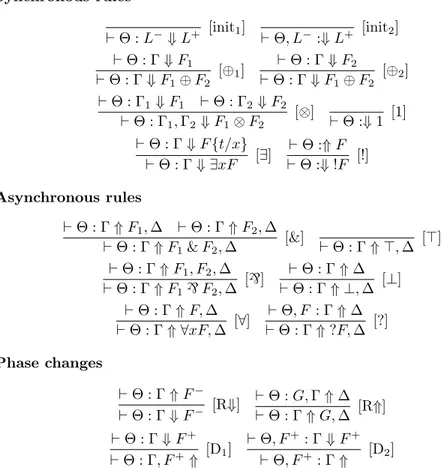
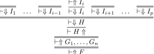
shows the focused proof system for linear logic. Sequents are of one of the two forms ⊢ Θ : Γ ⇓ F or ⊢ Θ : Γ ⇑ ∆. Those sequents should be read in the unfocused sequent calculus as ⊢ ?Θ, Γ, F and ⊢ ?Θ, Γ, ∆ respectively. Θ is a set of formulae, Γ is a multiset of positive formulae and negative literals, F is a formula, and ∆ is a multiset of formulae. A sequent of the form ⊢ Θ : Γ ⇓ F is in a synchronous phase, and focuses on the formula F . A sequent of the form ⊢ Θ : Γ ⇑ ∆ is in an asynchronous phase, and ∆ is the multiset of the potentially asynchronous formulae that need to be taken care of before the end of the phase.
The structure of focused proofs suggests abstracting away from the details of the phases. We may consider synchronous (resp. asynchronous) phases as large synthetic inference rules [Cur05] introducing a full layer of synchronous (resp. asynchronous) connectives. In particular, we will identify two focused proofs which only differ by a permutation of inference rules within a phase. It should be pointed out that although the order in which individual rules are
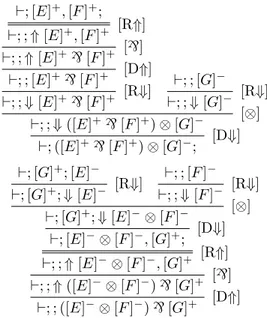
Synchronous rules ⊢ Θ : L− ⇓ L+ [init1] ⊢ Θ, L−:⇓ L+ [init2] ⊢ Θ : Γ ⇓ F1 ⊢ Θ : Γ ⇓ F1⊕ F2 [⊕1] ⊢ Θ : Γ ⇓ F2 ⊢ Θ : Γ ⇓ F1⊕ F2 [⊕2] ⊢ Θ : Γ1⇓ F1 ⊢ Θ : Γ2⇓ F2 ⊢ Θ : Γ1, Γ2⇓ F1⊗ F2 [⊗] ⊢ Θ :⇓ 1 [1] ⊢ Θ : Γ ⇓ F {t/x} ⊢ Θ : Γ ⇓ ∃xF [∃] ⊢ Θ :⇑ F ⊢ Θ :⇓ !F [!] Asynchronous rules ⊢ Θ : Γ ⇑ F1, ∆ ⊢ Θ : Γ ⇑ F2, ∆ ⊢ Θ : Γ ⇑ F1& F2, ∆ [&] ⊢ Θ : Γ ⇑ ⊤, ∆ [⊤] ⊢ Θ : Γ ⇑ F1, F2, ∆ ⊢ Θ : Γ ⇑ F1` F2, ∆ [`] ⊢ Θ : Γ ⇑ ⊥, ∆⊢ Θ : Γ ⇑ ∆ [⊥] ⊢ Θ : Γ ⇑ F, ∆ ⊢ Θ : Γ ⇑ ∀xF, ∆ [∀] ⊢ Θ, F : Γ ⇑ ∆ ⊢ Θ : Γ ⇑ ?F, ∆ [?] Phase changes ⊢ Θ : Γ ⇑ F− ⊢ Θ : Γ ⇓ F− [R⇓] ⊢ Θ : G, Γ ⇑ ∆ ⊢ Θ : Γ ⇑ G, ∆ [R⇑] ⊢ Θ : Γ ⇓ F+ ⊢ Θ : Γ, F+⇑ [D1] ⊢ Θ, F+ : Γ ⇓ F+ ⊢ Θ, F+: Γ ⇑ [D2]
F+ (resp. F−) stands for a positive (resp. negative) formula. L+ (resp. L−)
stands for a positive (resp. negative) literal. In [R⇑], G is either a positive formula or a negative literal.
applied is nondeterministic, there is only one asynchronous phase with a given conclusion. In other words, all the non-deterministic choices are grouped in synchronous phases, which does not come as a surprise since asynchronous rules are invertible. As we shall see in this thesis, focalisation is adapted to an interactive interpretation: a synchronous phase corresponds to choices that we make, and an asynchronous phase to choices that an opponent makes.
As we will mostly be interested in MALL, the proof systems we will con-sider will be simpler. The non-linear Θ zone is not needed in the absence of exponentials.
1.5
Multifocalisation
Although focalisation provides an abstraction from individual inference rules, it forces the decomposition of synchronous formulae to be sequentialised. The [D1] and [D2] rules start a synchronous phase by picking a formula as focus, and
the other synchronous formulae have to wait for their turn. Consider the two following MLL focused proofs.
⊢ L−⇓ L+ [init1] ⊢ L+, L−⇑ [D1] ⊢ L+⇑ L−` ⊥ [`, R⇑, ⊥] ⊢ L+⇓ (L−` ⊥) ⊗ 1 [⊗, R⇓, 1] ⊢ (L−` ⊥) ⊗ 1, L+⇑ [D1] ⊢ (L−` ⊥) ⊗ 1 ⇑ L+` ⊥ [`, R⇑, ⊥] ⊢ (L−` ⊥) ⊗ 1 ⇓ (L+` ⊥) ⊗ 1 [⊗, R⇓, 1] ⊢ (L+` ⊥) ⊗ 1, (L−` ⊥) ⊗ 1 ⇑ [D1] ⊢ L−⇓ L+ ⊢ L−, L+ ⇑ ⊢ L−⇑ L+` ⊥ ⊢ L−⇓ (L+` ⊥) ⊗ 1 ⊢ (L+` ⊥) ⊗ 1, L−⇑ ⊢ (L+` ⊥) ⊗ 1 ⇑ L−` ⊥ ⊢ (L+` ⊥) ⊗ 1 ⇓ (L−` ⊥) ⊗ 1 ⊢ (L+` ⊥) ⊗ 1, (L−` ⊥) ⊗ 1 ⇑
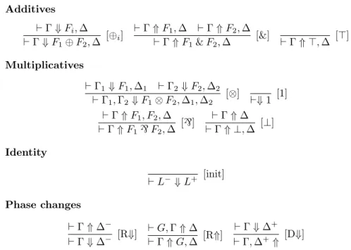
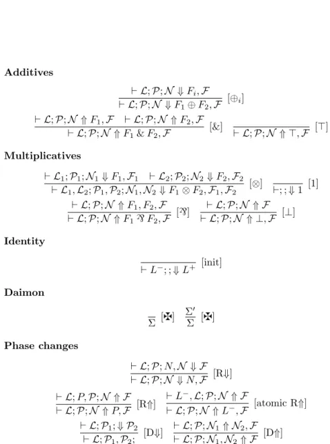
Those proofs only differ by the order in which the phases are scheduled. Chaud-huri, Miller and Saurin propose in [CMS08] to extend focalisation by allowing several foci to be selected for a synchronous phase, a feature known as mul-tifocalisation. They introduce a sequent calculus for MALL (see Figure 1.4). Saurin provides a multifocused sequent calculus for the full logic in [Sau08b]. Multifocused sequent calculus is clearly sound and complete with respect to LL. Soundness is seen by removing focusing annotations from sequents, and completeness follows from the completeness of single focalisation.
In addition to the two sequentialised proofs above, multifocusing allows a proof in which the synchronous formulae are decomposed concurrently:
⊢ L−⇓ L+ [init]
⊢ L+, L−⇑ [D]
⊢⇑ L+` ⊥, L−` ⊥ [`, R⇑, ⊥]
⊢⇓ (L+` ⊥) ⊗ 1, (L−` ⊥) ⊗ 1 [⊗, R⇓, 1]
⊢ (L+` ⊥) ⊗ 1, (L−` ⊥) ⊗ 1 ⇑ [D]
The authors of [CMS08] show that maximally multifocused MLL proofs cor-respond to MLL proof nets. We will not cover this topic here, but we will
Additives ⊢ Γ ⇓ Fi, ∆ ⊢ Γ ⇓ F1⊕ F2, ∆ [⊕i] ⊢ Γ ⇑ F1, ∆ ⊢ Γ ⇑ F2, ∆ ⊢ Γ ⇑ F1& F2, ∆ [&] ⊢ Γ ⇑ ⊤, ∆ [⊤] Multiplicatives ⊢ Γ1⇓ F1, ∆1 ⊢ Γ2⇓ F2, ∆2 ⊢ Γ1, Γ2⇓ F1⊗ F2, ∆1, ∆2 [⊗] ⊢⇓ 1 [1] ⊢ Γ ⇑ F1, F2, ∆ ⊢ Γ ⇑ F1` F2, ∆ [`] ⊢ Γ ⇑ ∆ ⊢ Γ ⇑ ⊥, ∆ [⊥] Identity ⊢ L− ⇓ L+ [init] Phase changes ⊢ Γ ⇑ ∆− ⊢ Γ ⇓ ∆− [R⇓] ⊢ G, Γ ⇑ ∆ ⊢ Γ ⇑ G, ∆ [R⇑] ⊢ Γ ⇓ ∆+ ⊢ Γ, ∆+⇑ [D⇓]
In [R⇑], G is either a positive formula or a negative literal. In [D⇓], ∆+ is not
empty.
Figure 1.4: Multifocalisation for MALL.
use multifocalisation as a way to improve the concurrency of focused sequent calculus.
1.6
Proof theory and computation
In the general context of the study of computation, approaches to proof theory traditionally fall into two categories.
In the computation-as-proof-normalisation approach, proofs model programs in functional languages. The computational content of this model is seen in the correspondence between proof normalisation and program execution. In that setting, a formula is a type, and a proof is a term of that type. A formula is true iff its type is not empty. Implication corresponds to the “arrow” constructor for types and plays a fundamental role. Proofs of A → B are functions mapping proofs of A to proofs of B. Proof normalisation corresponds to β-reduction in λ-calculus.
In the computation-as-proof-search approach, the state of the computation is seen as a sequent, and the computation itself as the search for a cut-free proof of that sequent. This is the basis for logic programming [MNPS91]. In that tradition, the specific features of a proof system are used to model proof search strategies. For example, the bias assignment to the atoms in a focused proof system can force forward-chaining or back-chaining [LM07].
1.7
Games and logic
The connections between logic and games have a long and rich history, although they remained informal until the 1950s. It is known since Aristotle that a debate can be seen as a game. The twentieth century saw the development of game theory, and connections were then made to logic. From the point of view of game theorists in general, the kinds of games studied in logic are quite specific. They typically involve two players with distinct roles, are not concerned with probabilities, and usually have two outcomes: a win for a player or for the opponent.
In a typical game for logic, the two players, called the Player and the Op-ponent, or ´Elo¨ıse and Ab´elard, build a sequence of moves called a play. For each finite sequence of moves, the rules of the game specify which player shall be the one to extend the sequence with a move, and which moves are at her disposal for doing so. Plays may be infinite in general, but there may also be some finite sequences of moves that cannot be extended with additional moves. In either case, the rules of the game classify maximal plays into those won by ´
Elo¨ıse and those won by Ab´elard. The plays are the uni-dimensional objects of the games. There are also bi-dimensional objects of interest called strategies. Strategies represent move policies that players may follow. A typical strategy is simply a set of plays that a player is prepared to follow. An important question about the game is whether a specific player can play according to some strategy which ensures her victory. If the answer is positive, then such strategies, called winning strategies, are formal witnesses to this fact. Similarly, proofs are wit-nesses to the truth of a formula. The games we are interested in tend to make this connection between games/formulae, provability/the existence of a winning strategy, proofs/winning strategies, and computation/dynamics of interaction.
Dialogue games were formalised by Lorenzen [Lor61]. In those games, the Player tries to establish the truth of a formula while the Opponent tries to establish its falsehood. Informally, the Opponent plays the role of an examiner and the Player plays the role of an examinee. For example, if the formula is a conjunction, the Opponent chooses a conjunct and challenges the Player to prove it; if it is a disjunction, the Player chooses which disjunct to prove.
Lorenzen’s work inspired mainstream game semantics in the computation-as-proof-normalisation tradition. The main idea is to interpret proofs as strategies, and to define an operation of composition of two strategies corresponding to the cut of the two proofs. This line of work began with Blass’ game semantics for linear logic [Bla92]. Major advances allowed to solve long-standing problems such as the full-abstraction problem for the language PCF [AJM00, HO00]. The objective was to establish a correspondence between strategies and programs, and this required controlling the information available to the players to choose moves. Hyland and Ong developed the adequate notion of innocent strategy to this end. Theses approaches also provided models for logics capturing the dynamics of cut elimination [AJ94, AM99]. Another major problem investigated in this line of research was the ability to represent concurrent programs in games. Abramsky and Melli`es developed concurrent games [AM99] in which moves are performed concurrently in maximal chunks. Melli`es also developed asynchronous games in which the traces of computation (sequences of moves) are equipped with a homotopy relation giving a geometric reading of concurrency. In this framework, it is possible to see innocence as positionality [Mel04].
Game-theoretical studies of logic programming are less common. Some of them model Prolog engines, beginning with [vE86] which connected Pro-log computations and two-person games using the αβ-algorithm. Loddo et al. [CLN98, Lod02] further developed this line of research with constraint logic programming [LC00]. Galanaki et al. [GRW08] accounted for negation in logic programming. Some other game-theoretic studies are more fundamentally con-cerned with proof search, as a foundation of logic programming. The games of Pym and Ritter [PR04] model the search for uniform proofs with backtrack-ing. More recently, Saurin [Sau08b, Sau08a] investigated proof search in Lu-dics [Gir01] guided by interaction with tests.
1.8
The neutral approach
The approach we develop in this thesis is inspired by dialogue games, but it clearly lies in the computation-as-proof-search tradition. The major novelty of this work is a change of perspective: instead of considering asymmetric settings in which the Player provides the arguments and the Opponent only aims at refuting them, we adopt a neutral approach with players having the same sta-tus. Both players attempt to prove a formula and to refute its negation. The computation can be seen as the simultaneous search for two orthogonal proofs, or dual proof search.
The neutral approach was first designed by Miller and Saurin in [MS06] in an essentially additive setting (see Chapter 2). A more subtle role assignment than the usual Player/Opponent dichotomy can be motivated by considering a common approach to proving the completeness of first-order classical logic, following, say, Smullyan [Smu95]. Proving completeness can be done by at-tempting to progressively build a sequent calculus derivation of a formula F . Each step extends the derivation with inference rules at the open leaves. If this is done in a systematic fashion, all the leaves are eventually closed, or the derivation ends up with a possibly infinite open branch. In the first case, there is a proof of F and in the second case, the open branch provides a falsifying model of F . This process can be seen as an interaction where one of the players attempts to complete the proof while the other one looks for an infinite branch. Exactly one of the players succeeds at their task.
This example relates the proof-theoretic notion of provability to the semantic notion of validity. In a decidable logic, models are expected to be finite, and so are the open branches of the derivation of F . In that case, it may be possible to extract a proof of ¬F from the counter-model for F read from an open branch. The interactive process would then be seen as two players building derivations of opposite formulae. However, models and proofs are objects which are different in nature and, even though the development of the derivation and of the counter-model of F are closely related at each step, there is no reason to expect the derivation of ¬F extracted from the counter-model to be related to the derivation of F .
The neutral approach solves this issue with a symmetric two-player game in which both players play with the same rules. If a player has a winning strategy, she is able to construct a proof: for one of the players, this would be a proof of F while dually for the other player, this would be a proof of ¬F . Each step extends the two orthogonal derivations with an inference rule of sequent calculus.
The core part of this thesis consists in defining neutral games for MALL. MALL has the advantage of having an extremely symmetric sequent calculus, which is required in our approach. The provability for MALL is PSPACE-complete, and MALL is incomplete. That is, there are formulae F such that neither F nor F⊥ are provable; take, for example, F = 1` 0. It means that the
neutral approach is not trivial in that logic: refuting a formula is not the same as proving its negation. Therefore, the game is not determinate: in some cases no player has a winning strategy. Some plays are not won by any player and, as a result, plays need to continue after one of the player has failed; it has yet to be determined whether the other player will win or not.
Chapter 3 presents a neutral game for MALL with a simple model in which the provability of a formula is equivalent to the existence of a winning strategy for the corresponding player. Chapter 4 switches to a radically different game model allowing for some concurrent behaviour, in which proofs are related to winning strategies.
Note that we follow a conventional angle. We aim at finding the suitable notion of game to bring the neutral approach to an existing logic with an existing notion of proof and refutation. In doing so, we stress the deep dualities of the logic, not only concerning proofs themselves, but also concerning the dynamics of proof search. The individual steps of proof search are performed simultaneously in the two orthogonal derivations. In contrast, Ludics [Gir01], while sharing some similarities with our work, takes another direction by radically departing from logic and making interaction the primitive notion.
Additive neutral games
This chapter introduces the neutral approach first developed by Miller and Saurin [MS06], restricting it to an additive setting in which refuting a formula is the same as proving its negation. Starting from a Hintikka-style dialogue game, we introduce a neutral syntax and discuss the remarkable properties that we wish to preserve in the game for MALL. In addition, we briefly revisit the sim-ple games, an extension to a fragment of MALL keeping this additive behaviour, yet expressive enough to encode numerous examples.
In the two-player games we consider, the players will be named 0 and 1. The symbol λ will typically denote a player. For every player λ ∈ {0, 1}, λ = 1 − λ will denote the opponent.
2.1
An additive neutral game
2.1.1
Hintikka’s additive game for truth
Jaakko Hintikka (see, for example, [Hod04]) presented a two player game to de-fine a notion of truth of a formula of first-order classical logic. One of Hintikka’s key observations was that playing on the negation of a formula F was the same as playing on F and exchanging the two players.
Two players, ´Elo¨ıse and Ab´elard, play on a single formula. ´Elo¨ıse tries to es-tablish the truth of the formula while Ab´elard tries to eses-tablish its falsehood. In this section, we present a propositional version of this game, using the propo-sitional additive fragment of linear logic (ALL). We recall the syntax of the formulae of this fragment:
F, G ::= F ⊕ G | 0 | F & G | ⊤
Hintikka’s original motivation was to provide an interactive definition of truth. In this presentation we take an alternate approach by switching to proof-theoretic notions. This distinction might seem shallow at first, since validity and provability are equivalent notions. However, seeing interaction as orthogonal proof search is at the heart of our approach, and applying this methodology to the richer MALL will provide insights into its proof theory.
The sequent calculus for ALL is straightforward: ⊢ Ei
⊢ E1⊕ E2
⊕i for i ∈ {1, 2} ⊢ E1 ⊢ E2
⊢ E1& E2 & ⊢ ⊤ ⊤
Formally, the game consists of an arena, which is a directed graph whose vertices, called positions, are the formulae occurrences, and whose arcs are called moves. Each move has an associated player, which can be either ´Elo¨ıse or Ab´elard. The following definition lists the moves of each player.
Definition 2.1.1. ´Elo¨ıse has two moves from every position of the form F ⊕ G, to F and G respectively. Ab´elard has two moves from every position of the form F & G, to F and G respectively.
We use the notation p → p′ to denote a move from a position p to a position
p′.
The positions from which there is no move, which are the occurrences of 0 and ⊤, are called terminal. A play p is a finite sequence p1, . . . , pn of positions
such that pi−1 → pi for 1 < i ≤ n. A play is maximal iff its last position is
terminal. A maximal play p1, . . . , pnis won by ´Elo¨ıse iff pn = ⊤, and by Ab´elard
iff pn = 0.
Informally, ´Elo¨ıse and Ab´elard discuss the truth of a formula by challenging each other. Each player aims at bringing the other player to a contradiction. Their argument is formally represented by a play, starting from the initial for-mula, and each move represents a step in the argument. When considering a disjunction F ⊕ G, ´Elo¨ıse gets to choose a disjunct with which to continue the discussion. Since she tries to establish the truth of F ⊕ G, and since F ⊕ G is true iff F is or G is, her task is to point out which one is. Ab´elard, who tries to establish that F ⊕ G is false, must be able to argue that F and G are both false. It seems therefore natural that ´Elo¨ıse be the one to make the choice between F and G: she simultaneously chooses which disjunct she believes to be true, and challenges Ab´elard to prove her wrong. Dually, when playing on a conjunction, Ab´elard is the one to make the choice between the conjuncts. When the play reaches a terminal position, representing the undeniable truth (⊤) or the undeniable falsehood (0), the player who is undeniably right wins the argument.
It is important to understand that there are, in general, many different plays starting from a given position, and that not all of them are won by the same player. In a real-life debate, someone defending a valid point may make some mistakes and end up losing an argument when confronted by a skilled opponent. Example 2.1.2. The tree of the plays starting at the true formula (⊤ ⊕ (0 ⊕ ⊤)) & ((0 & ⊤) ⊕ ⊤) is (⊤ ⊕ (0 ⊕ ⊤)) & ((0 & ⊤) ⊕ ⊤) ⊤ ⊕ (0 ⊕ ⊤) ⊤ 0 ⊕ ⊤ 0 ⊤ (0 & ⊤) ⊕ ⊤ 0 & ⊤ 0 ⊤ ⊤
Clearly, some of the maximal ones are won by ´Elo¨ıse, some others by Ab´elard. As illustrated by this example, a play is a uni-dimensional object which does not contain enough information to decide the truth of a formula. It is, however, a trace of a debate which ends with a player failing to prove her point. This does not come as a surprise, since objects establishing the truth of a formula, like proofs, are usually bi-dimensional. In games, a player sometimes has a way to play which ensure her victory, no matter how the opponent chooses to play.
A strategy is an object representing how a player is willing to play. A strategy is winning when the player wins all the terminal plays in which she follows the strategy. Strategies are bi-dimensional objects, formalised here as the set of plays the player is willing to play.
Definition 2.1.3 (Strategy). Let λ be a player. A λ-strategy for a position p is a minimal prefixed-closed set σ of plays such that:
• p ∈ σ,
• if p1, . . . , pn ∈ σ and player λ moves at pn, then there is exactly one
position pn+1 such that pn→ pn+1 and the play p1, . . . , pn+1 is in σ,
• if p1, . . . , pn ∈ σ and player λ moves at pn, then for every position pn+1
such that pn → pn+1, the play p1, . . . , pn+1 is in σ.
A λ-strategy is winning iff λ wins all its maximal plays.
Here we require strategies to be deterministic (whenever the player has to move, the strategy must specify at most one move) and total (whenever the player has to move, the strategy specifies at least one move; when the opponent has to move, the strategy accepts all possible moves).
In Example 2.1.2, ´Elo¨ıse has two winning strategies:
• one consisting of the plays (⊤ ⊕ (0 ⊕ ⊤)) & ((0 & ⊤) ⊕ ⊤), ⊤ ⊕ (0 ⊕ ⊤), ⊤ and (⊤ ⊕ (0 ⊕ ⊤)) & ((0 & ⊤) ⊕ ⊤), (0 & ⊤) ⊕ ⊤, ⊤, along with their prefixes;
• one consisting of the plays (⊤ ⊕ (0 ⊕ ⊤)) & ((0 & ⊤) ⊕ ⊤), ⊤ ⊕ (0 ⊕ ⊤), 0 ⊕ ⊤, ⊤ and (⊤ ⊕ (0 ⊕ ⊤)) & ((0 & ⊤) ⊕ ⊤), (0 & ⊤) ⊕ ⊤, ⊤, along with their prefixes.
Winning strategies allow a player to win against all attacks. The two play-ers cannot both have winning strategies at the same time. Otherwise playing them against each other would yield a play won by the two players, which is impossible. Not surprisingly, having a winning strategy means that the player playing it is correct at establishing the truth.
Theorem 2.1.4. Let E be a formula. E is true iff ´Elo¨ıse has a winning strategy for E. E is false iff Ab´elard has a winning strategy for E
Proof. If E = ⊤, ´Elo¨ıse has a trivial winning strategy. If E = 0, ´Elo¨ıse has no winning strategy. If E is of the form F ⊕ G, ´Elo¨ıse has a winning strategy iff she has a winning strategy for F or a winning strategy for G. If E is of the form F & G, ´Elo¨ıse has a winning strategy iff she has a winning strategy for F and a winning strategy for G. Those cases exactly match the truth semantics of the logic, hence the theorem. The dual result for Ab´elard is equally obvious.
Modelling truth is one of the objectives of the connections between logic and games, but we can do better. Since winning strategies are formal objects establishing the truth of a formula, it is natural to question how they relate to proofs. Depending on the game model and proof system, winning strategies may not correspond to proofs at all, correspond exactly to proofs, or correspond to classes of proofs.
In the case of our additive game, the correspondence is clearly one-to-one. Theorem 2.1.5. Let E be a formula. There is a one-to-one correspondence between the cut-free ALL proofs of E and ´Elo¨ıse’s winning strategies for E.
For example, ´Elo¨ıse’s winning strategies for Example 2.1.2 correspond to the two proofs of (⊤ ⊕ (0 ⊕ ⊤)) & ((0 & ⊤) ⊕ ⊤):
⊢ ⊤ ⊤
⊢ ⊤ ⊕ (0 ⊕ ⊤) ⊕1
⊢ ⊤ ⊤
⊢ (0 & ⊤) ⊕ ⊤ ⊕2 ⊢ (⊤ ⊕ (0 ⊕ ⊤)) & ((0 & ⊤) ⊕ ⊤) & and ⊢ ⊤ ⊤ ⊢ 0 ⊕ ⊤ ⊕2 ⊢ ⊤ ⊕ (0 ⊕ ⊤) ⊕2 ⊢ ⊤ ⊤ ⊢ (0 & ⊤) ⊕ ⊤ ⊕2 ⊢ (⊤ ⊕ (0 ⊕ ⊤)) & ((0 & ⊤) ⊕ ⊤) &
Remark 2.1.6. In sequent calculus, the two proofs of ⊢ ⊤ ⊕ ⊤ are distinct. We define the positions of the game as formula occurrences instead of plain formulae to make the same distinction. Otherwise the two disjuncts of ⊤ ⊕ ⊤ would be identified and ´Elo¨ıse would only have one winning strategy for this formula.
2.1.2
A neutral presentation
An important feature of ALL is its completeness. For every formula E, either E or E⊥is provable. Making this observation explicit in sequent calculus is not
easy, but it can be done in the game. The game is symmetric in the sense that disjunction (⊕ and 0) is treated in the same way by ´Elo¨ıse as conjunction (& and ⊤) by Ab´elard. What matters is not the current formula in a play, but who plays. If we negate all formulae in a game, the strategies of ´Elo¨ıse and Ab´elard are swapped.
Corollary 2.1.7. Let E be a formula. There is a one-to-one correspondence between the proofs of E⊥ and Ab´elard’s winning strategies in E.
This is a stronger statement than the mere completeness of the logic: not only is E⊥ provable if and only if E is not, but the refutations of E (witnesses
that it is unprovable) are in one-to-one correspondence with the proofs of E⊥.
Therefore, the game can be seen as the simultaneous development of two dual derivations, in which ´Elo¨ıse attempts to derive E while Ab´elard attempts to derive E⊥. Both derivations are built from the bottom up. Whenever one of
the players faces a sequent of the form ⊢ F1⊕ F2, she picks one of the disjuncts
Fi by extending the derivation with the rule ⊕i. Simultaneously her opponent
faces ⊢ F1⊥& F2⊥ and, depending on the choice of her opponent, is challenged
to prove either ⊢ F⊥
1 or ⊢ F2⊥. Even if only one of the conjuncts is picked
during a given play, the opponent must be able to accommodate to any of the two choices of the player, and her winning strategies are indeed composed of two separate sub-strategies, exactly like the proofs of ⊢ F⊥
1 & F2⊥. Whenever
one of the players faces ⊢ ⊤, she can close her derivation and wins; while her opponent, who faces ⊢ 0, cannot close her derivation and loses.
Note that since a given play only explores one branch of each conjunction, it is not a derivation per se, rather an additive slice of a derivation.
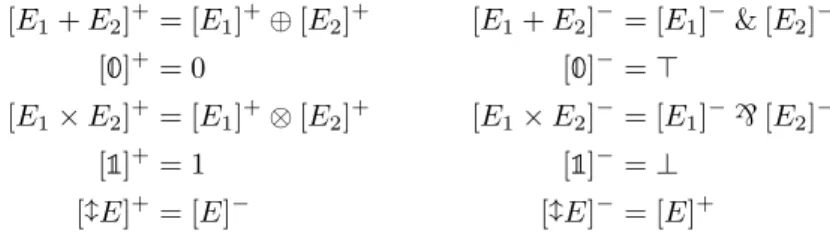
This duality motivates the introduction of a neutral syntax replacing that of formulae. Conjunction and disjunction will be replaced by a single neutral connective +, its unit will be denoted to by✵, and we will denote the change of player by˜.
[E1+ E2]+= [E1]+⊕ [E2]+ [E1+ E2]−= [E1]−& [E2]−
[✵]+= 0 [✵]−= ⊤
[˜E]+= [E]− [˜E]−= [E]+
Figure 2.1: Positive and negative translations of additive neutral expressions into ALL.
Definition 2.1.8 (Additive neutral expressions). The additive neutral expres-sions E and guarded additive neutral expresexpres-sions G are inductively defined as follows.
G, G′::= E + E′|✵ E, E′::= G |˜G
An additive neutral expression can be seen as a pair of two dual formulae of ALL called its positive and negative translations. Figure 2.1 defines them.
We can now reformulate the game in terms of neutral expressions instead of formulae.
Definition 2.1.9 (Propositional additive game). The game on a neutral ex-pression E consists of positions and moves. The positions are the occurrences of the sub-expressions of E. Consider the rewrite rules
E1+ E27→ E1 E1+ E27→ E2
There is a move E → F iff E 7→∗ ˜F . A position from which there is no move
is terminal. Plays are defined as before.
Definition 2.1.10(Strategy). A strategy for a position p is a minimal prefixed-closed set σ of plays such that:
• p ∈ σ,
• if p1, . . . , pn ∈ σ is not maximal and n is odd, then there is exactly one
position pn+1 such that pn→ pn+1 and the play p1, . . . , pn+1 is in σ,
• if p1, . . . , pn ∈ σ is not maximal and n is even, then for every position
pn+1 such that pn → pn+1, the play p1, . . . , pn+1 is in σ.
A strategy is winning iff all its maximal plays have even length, and counter-winning iff all its maximal plays have odd length.
Theorem 2.1.11. Let E be a neutral expression. There is a one-to-one corre-spondence between the proofs of [E]+ and the winning strategies for E. There is
a one-to-one correspondence between the proofs of [E]− and the counter-winning
strategies for E.
Additive behaviour is well captured by this game, with the benefit of im-proved symmetry. In Hintikka’s game, the same player might move several times in a row, as long as the principal connective of the formula remains the same. In our game these moves correspond to individual rewrite steps and a move is a maximal sequence of such steps, which ensures a strict alternation of players. From the point of view of the proof objects, a rewrite step (a.k.a. a micro-move)
corresponds to the introduction of an individual connective or unit, while a move (a.k.a. a macro-move) corresponds to a full phase. The games for MALL we develop in the next chapters are more complex but their moves still have those two levels.
With this neutral syntax it is even clearer that this game may be seen as a process accounting for the simultaneous development of two dual derivations: starting from a neutral expression E, the player who begins sees the game as an attempt to derive ⊢ [E]+, while her opponent sees it as an attempt to derive
⊢ [E]−. With this in mind, each player develops what she sees as synchronous
phases during her turn and leaves it to her opponent to decompose asynchronous phases.
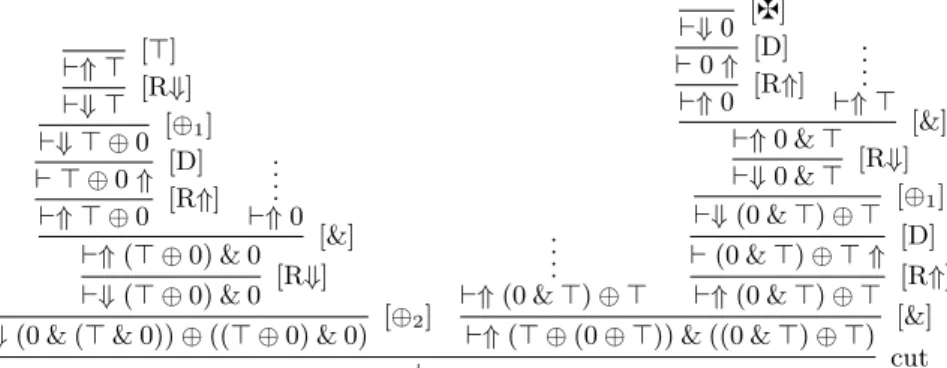
Let us revisit Example 2.1.2 and describe it in terms of neutral expressions. The formula (⊤⊕(0⊕⊤))&((0&⊤)⊕⊤) is replaced with the neutral expression ˜(˜✵ + (✵ + ˜✵)) + ˜(˜(˜✵ + ✵) + ˜✵), of which it is the negative translation. We draw the tree of plays starting from this neutral expression:
˜(˜✵ + (✵ + ˜✵)) + ˜(˜(˜✵ + ✵) + ˜✵) ˜✵ + (✵ + ˜✵) ✵ ✵ ˜(˜✵ + ✵) + ˜✵ ˜✵ + ✵ ✵ ✵
In the original game, Ab´elard was the one to begin and ´Elo¨ıse had winning strategies. Therefore the winning player was the one who did not start. It must also be the case in the neutral version of the game. In our terminology, there is a counter-winning strategy.
In the neutral game, there is a strict alternation of players. In contrast, ´Elo¨ıse would play twice in a row at ⊤ ⊕ (0 ⊕ ⊤) in the original game, for example. Those possible sequences of moves by ´Elo¨ıse are replaced in the neutral game with the macro-moves from ˜✵ + (✵ + ˜✵) to ✵ and ✵ (distinct occurrences). Those macro-moves correspond respectively to the sequences of micro-moves ˜✵ + (✵ + ˜✵) 7→ ˜✵ and ˜✵ + (✵ + ˜✵) 7→ ✵ + ˜✵ 7→ ˜✵. Since players alternate strictly, the parity of the length of a maximal play determines its winner.
There are two counter-winning strategies, corresponding to the two winning strategies of ´Elo¨ıse in the original game. The first one is composed of the plays ˜(˜✵ + (✵ + ˜✵)) + ˜(˜(˜✵ + ✵) + ˜✵), ˜✵ + (✵ + ˜✵), ✵ and ˜(˜✵ + (✵ + ˜✵)) + ˜(˜(˜✵ + ✵) + ˜✵), ˜(˜✵ + ✵) + ˜✵, ✵. Its corresponding proof is, unsurprisingly, the same as the one corresponding to the original winning strategy. If we rewrite it in a focused proof system
⊢⇑ ⊤ [⊤] ⊢⇓ ⊤ [R⇓] ⊢⇓ ⊤ ⊕ (0 ⊕ ⊤) [⊕1] ⊢ ⊤ ⊕ (0 ⊕ ⊤) ⇑ [D] ⊢⇑ ⊤ ⊕ (0 ⊕ ⊤) [R⇑] ⊢⇑ ⊤ [⊤] ⊢⇓ ⊤ [R⇓] ⊢⇓ (0 & ⊤) ⊕ ⊤ [⊕2] ⊢ (0 & ⊤) ⊕ ⊤ ⇑ [D] ⊢⇑ (0 & ⊤) ⊕ ⊤ [R⇑] ⊢⇑ (⊤ ⊕ (0 ⊕ ⊤)) & ((0 & ⊤) ⊕ ⊤) [&]
it becomes clear that micro-moves are read as individual inference rules while macro-moves are read as phases. Synchronous phases are macro-moves by the player, and asynchronous phases are macro-moves by the opponent. The intro-duction of focalisation in ALL for this single remark may seem overkill, even more so because focalisation is trivial in that context. The abstraction provided by focalisation will prove useful when we introduce multiplicatives in the game.
2.1.3
Computation as dual proof search
In the above example, the player who starts does not have a winning strategy. Determining it requires to explore the arena much like a search space in proof search. This graph exploration progressively partitions the positions in two sets, starting from the terminal ones, depending on which player has a winning strategy for them. This process not only does this classification, but it also builds winning strategies. Since steps in the game (micro-moves and macro-moves) correspond to steps in proofs (rules and phases), it is clear that the exploration of the arena builds derivations gradually. In this respect, this game is deeply rooted in the tradition of computation as proof search. An interesting aspect of this computation is that we always get a winning strategy in the end (hence a proof), but we do not know for which player until we finish. Hence, the computation can be seen as the simultaneous development of two dual derivations, one of which will eventually be closed to become a proof.
In the above example, the maximal play˜(˜✵ + (✵ + ˜✵)) + ˜(˜(˜✵ + ✵) + ˜✵), ˜(˜✵ + ✵) + ˜✵, ˜✵ + ✵, ✵ is seen as two dual derivation slices. From the point of view of the player who begins—and attempts to prove (0 & (⊤ & 0)) ⊕ ((⊤ ⊕ 0) & 0)—, the play corresponds to the slice
⊢⇑ ⊤ [⊤] ⊢⇓ ⊤ [R⇓] ⊢⇓ ⊤ ⊕ 0 [⊕1] ⊢ ⊤ ⊕ 0 ⇑ [D] ⊢⇑ ⊤ ⊕ 0 [R⇑] ⊢⇑ (⊤ ⊕ 0) & 0 [&1] ⊢⇓ (⊤ ⊕ 0) & 0 [R⇓]
⊢⇓ (0 & (⊤ & 0)) ⊕ ((⊤ ⊕ 0) & 0) [⊕2]
while from the point of view of the player who does not begin—and attempts to prove (⊤ ⊕ (0 ⊕ ⊤)) & ((0 & ⊤) ⊕ ⊤)—, the play corresponds to the slice
⊢⇓ 0 [z] ⊢ 0 ⇑ [D] ⊢⇑ 0 [R⇑] ⊢⇑ 0 & ⊤ [&1] ⊢⇓ 0 & ⊤ [R⇓] ⊢⇓ (0 & ⊤) ⊕ ⊤ [⊕1] ⊢ (0 & ⊤) ⊕ ⊤ ⇑ [D] ⊢⇑ (0 & ⊤) ⊕ ⊤ [R⇑]
⊢⇑ ⊤ [⊤] ⊢⇓ ⊤ [R⇓] ⊢⇓ ⊤ ⊕0 [⊕1] ⊢ ⊤ ⊕0 ⇑ [D] ⊢⇑ ⊤ ⊕0 [R⇑] .. .. ⊢⇑0 ⊢⇑(⊤ ⊕ 0) & 0 [&] ⊢⇓(⊤ ⊕ 0) & 0 [R⇓]
⊢⇓(0 & (⊤ & 0)) ⊕ ((⊤ ⊕ 0) & 0) [⊕2]
.. .. ⊢⇑(0 & ⊤) ⊕ ⊤ ⊢⇓0 [z] ⊢0 ⇑ [D] ⊢⇑0 [R⇑] .. .. ⊢⇑ ⊤ ⊢⇑0 & ⊤ [&] ⊢⇓0 & ⊤ [R⇓] ⊢⇓(0 & ⊤) ⊕ ⊤ [⊕1] ⊢(0 & ⊤) ⊕ ⊤ ⇑ [D] ⊢⇑(0 & ⊤) ⊕ ⊤ [R⇑] ⊢⇑(⊤ ⊕ (0 ⊕ ⊤)) & ((0 & ⊤) ⊕ ⊤) [&]
⊢ cut
Figure 2.2: Two dual derivations cut together. We have omitted the details of the derivations/strategies that will not be explored by the cut elimination procedure/in the play resulting from the interaction.
which we closed with the special rule daimon [z], named by analogy with Lu-dics [Gir01]. This rule stands for a “joker” allowing to close any branch. Of course, a derivation using the daimon is not a proof, but it is still an interesting object for our purpose. Here this rule is used as evidence that the branch cannot be closed, and plays a dual role to [⊤], which is applied by the other player. It does not come as a surprise that the winner of the play closes her branch legally with [⊤] and that the loser closes it with [z].
This observation can be generalised to two-dimensional objects: strategies and closed derivations. The exploration of the arena is seen as the simultane-ous development of two dual derivations. A strategy corresponds to a closed derivation, and a strategy is winning iff its derivation does not use [z] i.e. is a proof.
2.1.4
Interaction as proof normalisation
Another approach to the computational content of this game is to view a play as the result of the interaction of two strategies. In proof-theoretic terms, two dual derivations interact with each other through cut elimination. For example, going back to our favourite example, let us consider the play˜(˜✵ + (✵ + ˜✵)) + ˜(˜(˜✵ + ✵) + ˜✵), ˜(˜✵ + ✵) + ˜✵, ✵ once again. We can complete the two slices given in the previous section to obtain derivations representing strategies for each player, and cut them together. Figure 2.2 shows the obtained derivation.
The admissibility of cut states that no proof of the empty sequent can exist. However, with the [z] rule, closed derivations of the empty sequent do exist. In game theoretic terms, this condition expresses that it is impossible for both players to have a winning strategy for the same position.
Clearly, the cut elimination procedure maintains the invariant that two dual closed derivations are cut together to infer the empty sequent, and the successive pairs of dual formulae being cut form the two slices presented before, or, in game theoretic terms, the play resulting from the interaction of the two strategies.
This observation relates the game to the tradition of computation as proof normalisation. The computational content of interaction lies in the cut
elimi-[E1+ E2]+= [E1]+⊕ [E2]+ [E1+ E2]−= [E1]−& [E2]−
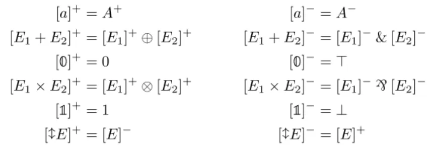
[✵]+= 0 [✵]−= ⊤
[E1× E2]+= [E1]+⊗ [E2]+ [E1× E2]−= [E1]−` [E2]−
[✶]+= 1 [✶]−= ⊥
[˜E]+= [E]− [˜E]−= [E]+
Figure 2.3: Positive and negative translations of additive and multiplicative neutral expressions into MALL.
nation procedure.
2.2
Simple games for a fragment of MALL
Our objective is to define a neutral game with not only additive but also mul-tiplicative behaviour. In [MS06] the authors investigate such a game for a fragment of multiplicative and additive linear logic. In that fragment, mul-tiplicatives of opposite polarities (⊗ and `) are not allowed to interact. We present a slight variation of that fragment here. It is considerably simpler to handle than MALL. Again, we restrict our presentation to the propositional case.
Neutral expressions are extended to incorporate a multiplicative connective × and its unit✶. Figure 2.3 shows their translations into MALL.
G, G′ ::= E + E′|✵ | E × E′ |✶
E, E′ ::= G |˜G
The fragment to which our study is restricted is presented further down. In the additive case, sequents only consisted of one formula. Positive and negative phases were of the form
Positive phase Negative phase
⊢⇑ [Gk]− ⊢⇓Ln i=1[Gi]− {⊢ [Gi]+⇑|1 ≤ i ≤ n} ⊢⇑˘ni=1[Gi]+ for some k ∈ {1, . . . , n}.
Plays correspond to additive slices, which consist of a single branch. We want to keep the same additive structure to the game, only introducing multiplicatives inside phases. A slice of a phase is allowed at most one premise, which must be a sequent with at most one formula. In other words, a positive phase needs to be either of the form
⊢⇓ G1 . . . ⊢⇓ Gi−1
⊢⇑ H
⊢⇓ Gi ⊢⇓ Gi+1 . . . ⊢⇓ Gn
or of the form
⊢⇓ G1 . . . ⊢⇓ Gn
⊢⇓ F
and a slice of a negative phase needs to be of one of the forms ⊢ H ⇑ ⊢⇑ G1, . . . , Gn ⊢⇑ F ⊢ ⊢⇑ G1, . . . , Gn ⊢⇑ F ⊢⇑ G1, . . . , Gn ⊢⇑ F With this restriction, derivations have the following shape:
• in positive phases, there are one or more branches and sequents contain exactly one formula;
• in negative phase slices, there is exactly one branch; the sequent contains zero or more formulae.
This particular shape suggests using multisets of neutral expression occur-rences to represent the state of a game in this fragment. A multiset {E1, . . . , En}
will be read positively as the collection of sequents ⊢⇓ [E1]+,. . . ,⊢⇓ [En]+ and
negatively as the sequent ⊢⇑ [E1]−, . . . , [En]−.
The micro-moves of the game are the following rewrite steps on multisets of neutral expression occurrences:
Γ,✶ 7→ Γ Γ, E1× E27→ Γ, E1, E2
Γ, E1+ E27→ Γ, E1 Γ, E1+ E27→ Γ, E2
where the comma denotes the multiset union.
Rewriting terminates since the total number of symbols of the neutral ex-pressions in a multiset strictly decreases. Neutral exex-pressions of the form ˜G do not rewrite (they are to be passed to the other player), and neither does ✵.
The restriction we want to impose on the logic corresponds to neutral expres-sions which yield, through rewriting, multisets containing at most one neutral expression of the form˜G. Formally, we define a measure ♮(E) representing the maximal number of neutral expressions of the form ˜G in a multiset that can be obtained from E through rewriting.
♮(✵) = ♮(✶) = 0 ♮(E1+ E2) = max(♮(E1), ♮(E2))
♮(˜G) = 1 ♮(E1× E2) = ♮(E1) + ♮(E2)
Definition 2.2.1(Simple neutral expressions). A neutral expression E is sim-ple iff ♮(E) ≤ 1 and all sub-expressions of E are simsim-ple.
Alternatively, simple neutral expressions E and guarded simple neutral ex-pressions G are defined with the following grammar:
Z, Z′::= Z + Z′|✵ | Z × Z′ |✶ G ::= Z | E × Z | Z × E E ::= G |˜G
We can now define the arena of the game.
Definition 2.2.2. The positions are the simple neutral expression occurrences. If {E} 7→∗{}, then there is a macro-move from E to✵. If {E} 7→∗{˜E′}, then