1
Introduction
European Union Allowances (EUAs) and Certified Emissions Reductions (CERs) are fungible assets within the European Union Emissions Trad-ing Scheme. Their properties have been documented by previous literature. First, Chevallier (2010) analyzes both time series in a vector autoregressive (VAR), impulse response function (IRF) and cointegrating framework. The author shows that EUAs and CERs affect each other significantly through the VAR model, and react quite rapidly to shocks on each other through the IRF analysis. Most importantly, both price series are found to be coin-tegrated, with EUAs leading the price discovery process in the long-term through the vector error-correction mechanism.
Second, Chevallier (2011) studies the time-varying correlations between the two assets in a Dynamic Conditional Correlation (DCC) GARCH model. The study confirms the presence of strong ARCH and GARCH effects, and documents correlations in the range of [0.01;0.90] between EUAs and CERs. These findings can then be re-used by financial agents to reach optimal risk management, portfolio selection, and hedging strategies.
Third, Mansanet-Bataller et al. (2011) investigate the price differences between EUAs and sCERs, and the extent to which financial and indus-trial operators may benefit from arbitrage strategies by buying sCERs and selling EUAs (i.e. selling the EUA-sCER spread). The authors show that the spread is mainly driven by EUA prices and market microstructure vari-ables, and less importantly by emissions-related fundamental drivers. This empirical analysis of emissions markets reveals the rational behavior of in-vestors: profit-maximizing strategies are elaborated given the very unusual institutional characteristics of emissions markets.
Compared to previous literature, this paper provides the first assessment of the interactions between EUAs and CERs in a Markov regime-switching environment. Given the recent changes in the underlying business cyle (i.e. a conjunction of a financial crisis since late 2007 coupled with a timid eco-nomic recovery since 2010), this approach may be beneficial to three groups of agents. On the one hand, academics would benefit from a greater un-derstanding of how the relationship between EUAs and CERs changes de-pending on economic activity. This literature has been documented for most energy markets (including the oil market), but to a lesser extent for the
carbon market.
On the other hand, regulatory authorities could also be interested in understanding how the price path of EUAs and CERs evolves during pe-riods of economic recession/expansion. If the carbon market is to exhibit clear macroeconomic fundamentals, then the regulator needs to diminish its intervention by amending the allocation rules for instance.
Finally, analysts, investment bankers and portfolio managers are inter-ested into the evolution of EUAs and CERs depending on the business cycle. Based on that information, they can formulate recommendations on buy/sell strategies, on the creation of new financial products, and on asset allocation strategies. If EUAs and CERs are found to be counter-cyclical for instance, then these emissions assets can be included for diversification purposes in a broad portfolio composed of equities, bonds and commodities.
Our main results highlight significant switches from low-growth to high-growth periods between the two time series, with the main regime switch being located in July 2009. Therefore, emissions assets are related to the underlying business cycle. Besides, EUAs affect CERs during expansions and recessions, while CERs are found to affect EUAs at statistically significant levels especially during expansions.
The rest of the paper is structured as follows. Section 2 summarizes the data used. Section 3 introduces the Markov regime-switching model. Section 4 presents the empirical results. Section 5 briefly concludes.
2
Data
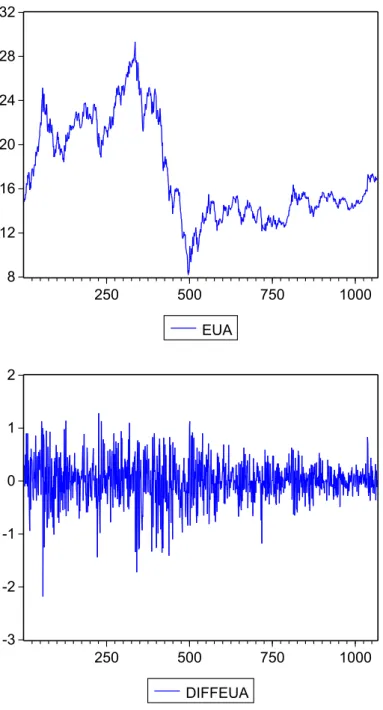
Figure 1 presents the daily time series of EUA Futures prices traded in Euro/ton of CO2 on the European Climate Exchange (ECX) from March 09,
2007 to April 26, 2011 which corresponds to a sample of 1,066 observations. The EUA Futures prices are also presented in logreturn transformation in the bottom panel of Figure 1.
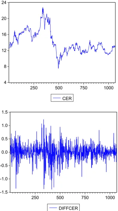
Figure 2 presents the daily time series of CER Futures prices traded in Euro/ton of CO2 on ECX. The start of the study periods corresponds to
the trading of CER futures allowances on ECX. The CER Futures prices are also presented in logreturn transformation in the bottom panel of Figure 2.
3
Regime-switching model
Following Hamilton (1989), time series may be modelled by following differ-ent processes at differdiffer-ent points in time, with the shifts between processes determined by the outcome of an unobserved Markov chain. In this frame-work, the presence of multiple regimes can be acknowledged using multivari-ate models where parameters are made dependent on a hidden stmultivari-ate process. Consider an n-dimensional vector yt ≡ (y1t, . . . , ynt)′ which is assumed to
follow a VAR(p) with parameters:
yt=µ(st) + p X i=1 Φi(st)yt−i+ ǫt ǫt∼ N (0, Σ(st)) (1)
where the parameters for the conditional expectation µ(st) and Φi(st),
i = 1, . . . , p, as well as the variances and covariances of the error terms ǫt in
the matrix Σ(st) all depend upon the state variable st which can assume a
number q of values (corresponding to different regimes). Given initial values for the regime probabilities, and the conditional mean for each state, the log-likelihood function can be constructed and maximised numerically to obtain parameters estimates of the model.
The general idea behind the class of Markov-switching models is that the parameters and the variance of an autoregressive process depend upon an unobservable regime variable st ∈ {1, . . . , M }, which represents the
proba-bility of being in a particular state of the world. A complete description of the Markov-switching model requires the formulation of a mechanism that governs the evolution of the stochastic and unobservable regimes on which the parameters of the autoregression depend. Once a law has been specified for the states st, the evolution of regimes can be inferred from the data.
Typically, the regime-generating process is an ergodic Markov chain with a finite number of states defined by the transition probabilities:
pij = P rob(st+1= j|st= i), M
X
j=1
In such a model, the optimal inference about the unobserved state vari-able st would take the form of a probability. The transition probabilities
of the Markov-process determines the probability that volatility will switch to another regime, and thus the expected duration of each regime. We rely on a constant specification to keep the model parsimonious. Each regime is thus the realization of a first-order Markov chain with constant transition probabilities.
By setting S = [1 1], both the autoregressive coefficients and the model’s variance are switching according to the transition probabilities. Typically, we set the number of states M equal to 2. Therefore, state M = 1 represents the ‘high growth’ phase, whereas state M = 2 characterizes the ‘low growth’ phase (for more details, see Hamilton (2008) and references therein). When M = 1, the growth of the endogenous variable is given by the population parameter µ1, whereas when M = 2, the growth rate is µ2.
As M rises, it becomes increasingly easy to fit complicated dynamics and deviations from the normal distribution in the returns (Guidolin and Tim-mermann (2006)). However, this comes at the cost of having to estimate more parameters. As Bradley and Jansen (2004) put it, a well-known prob-lem with any application of nonlinear models is the probprob-lem of overfitting. There is therefore a trade-off between the depth of the economic interpreta-tion which one would have available with higher degrees for state variables, and the numerical difficulties which accompany such an effort.
The model is estimated based on Gaussian maximum likelihood with St = 1, 2. The calculation of the covariance matrix is performed using the
second partial derivatives of the log likelihood function. P is the transition matrix which controls the probability of a switch from state M = 1 to state M = 2: P = " p11 p21 p12 p22 #
The sum of each column in P is equal to 1, since they represent the full probabilities of the process for each state.
4
Empirical results
4.1 Comments
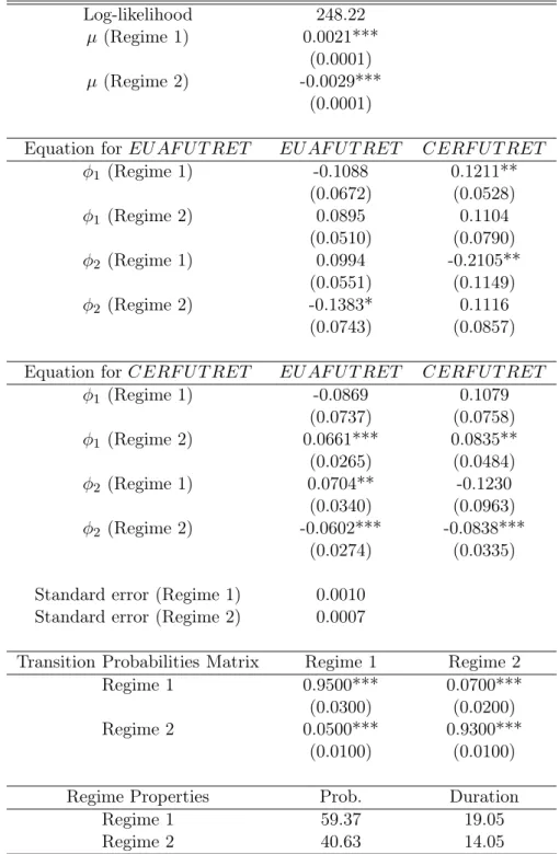
Results are provided in Table 3. The statistically significant coefficients of the two means µ show the presence of switches between high-/low-growth periods. During expansion, output growth per month is equal to 0.21% on average. The time series is likely to remain in the expansionary phase with an estimated probability equal to 95%. Regime 1 is assumed to last 19 days on average. During recession, the average growth rate is equal to -0.29%. The probability that it will stay in recession is equal to 93%. The average duration of Regime 2 is 14 days. According to the ergodic probabilities, the time series would spend 60% (40%) of the time spanned by our data sample in Regime 1 (Regime 2).
Interestingly, other coefficient estimates suggest that EUAs have several statistically significant effects on EUAs: during Regime 1 (as φ2 = 0.07
is significant at the 5% level), and during Regime 2 (as φ1 = 0.06 and
φ2 = −0.06 are significant at the 1% level). Therefore, these results confirm
the insights by Chevallier (2010, 2011) concerning the significant impact of EUAs on CERs, since the EU ETS is the most developed emissions market in the world to date. Concerning CERs, we can notice that they impact EUAs essentially during expansionary phases (as φ1 = 0.12 and φ2= −0.21
are significant at the 5% level).
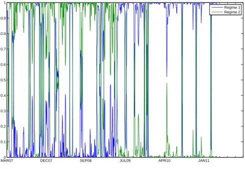
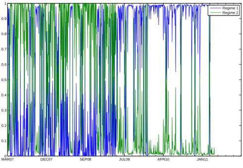
The associated smoothed and regime probabilities1 are shown in Figures
3 and 4, respectively. They reveal essentially two periods in the carbon futures markets: a low-growth period during March 2007-June 2009, and a high-growth period during July 2009-April 2011. The main switch from regime 2 to regime 1 occurs during July 2009, as the world economies start to recover from the financial crisis. Therefore, the Markov-switching model reveals new characteristics about the behaviour of emissions assets.
1The estimation routine generates two by-products in the form of the regime and smooth
probabilities. Recall that the regime probability at time t is the probability that state t will operate at t, conditional on information available up to t − 1. The other by-product is the smooth probability, which is the probability of a particular state in operation at time t conditional on all information in the sample. The smooth probability allows the researcher to ‘look back’ and observe how regimes have evolved overtime.
4.2 Diagnostic tests
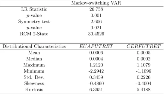
The upper panel of Table 4 reports the results of three diagnostic tests. The first is a test of the Markov-switching model against the simple nested null hypothesis that the data follow a geometric random walk with i.i.d innovations. Note M the p-value from the LR test:
P rob[LR(q∗)] > M = P rob(χ2
d> M ) +
V M(d−1)/2e−M/22−d/2
Γ(d/2) (3)
where P rob(LR(q∗) > M |H
0) is the upper bound critical value, LR
is the likelihood ratio statistic, q∗ is the vector of transition probabilities
(q∗= argmax LnL(q)|H
1) and d is the number of restrictions under the null
hypothesis.
In Table 4, this adjustment produces a LR statistic equal to 26.75. We reject the random walk at the 0.1 percent level. We conclude that the rela-tionship is better described by a two-regime Markov-switching model than by the random walk model.
The second test reported in Table 4 is for symmetry of the Markov tran-sition matrix, which implies symmetry of the unconditional distribution of the growth rates. This test examines the maintained hypothesis that p (the probability of being in a high-growth state or boom) equals q (the probabil-ity of being in a low-growth state or depression) against the alternative that p < q. Table 4 reports statistics that are asymptotically standard normal under the null. We reject the hypothesis of symmetry at the 5% level.
Third, Ang and Bekaert (2002) set out a formal definition of and a test for regime classification. They argue that a good regime switching model should be able to classify regimes sharply. Weak regime inference implies that the regime-switching model cannot successfully distinguish between regimes from the behavior of the data, and may indicate misspecification. To measure the quality of regime classification, we therefore use Ang and Bekaert’s (2002) Regime Classification Measure (RCM) defined for two states as:
RCM = 400 × 1 T T X t=1 pt(1 − pt) (4)
and 100, and pt denotes the ex-post smoothed regime probabilities. Good
regime classification is associated with low RCM statistic values. A value of 0 indicates that the two-regime model is able to perfectly discriminate between regimes, whereas a value of 100 indicates that the two-regime model simply assigns each regime a 50% chance of occurrence throughout the sample. Consequently, a value of 50 is often used as a benchmark (see Chan et al. (2011) for instance).
Adopting this definition to the current context, the RCM 2-State statistic is equal to 30.45 in Table 4. It is substantially below 50, consistent with the existence of two regimes. It is very interesting that our estimated Markov-switching model has classified the two regimes extremely well.
Finally, Table 4 reports the distributional characteristics for the Markov-switching processes implied by the estimates in Table 3. Compared to Tables 1 and 2, these values demonstrate that the two-regime model we employ matches quite well the first four central moments of the data. We conclude that the Markov-switching model produces both the degree of skewness and the amount of kurtosis that are present in the original data.
5
Conclusion
The main idea behind Markov regime-switching models consists in capturing the behavior of economic time series with respect to the underlying business cycle. Since the years 2007 to 2011 have been characterized by periods of economic growth and recession, it appears interesting to investigate how the interactions between EUAs and CERs - the two most fungible assets among emissions markets - evolve in this context.
This paper shows that significant interactions exist between the two mar-kets, especially during periods of economic recession when the market trends are destabilised. Besides, EUAs and CERs seem to vary during two main periods from low-growth to high-growth, with the main regime switch occur-ing in July 2009 (in the recovery process from the financial crisis). Overall, the Markov-Switching modelling brings us new insights as to when market shocks occur, and actually impact the EUA and CER futures price series. Thefeore, the results presented in this paper can be seen as complementary to the time-varying correlations between the two markets highlighted recently by Chevallier (2011).
References
Ang, A., Bekaert, G. 2002. Regime Switches in Interest Rates. Journal of Business and Economic Statistics 20(2), 163-182.
Bradley, M.D., Jansen, D.W. 2004. Forecasting with a nonlinear dynamic model of stock returns and industrial production. International Journal of Forecasting 20(2), 321-342.
Chan, K.F., Treepongkaruna, S., Brooks, R., Gray, S. 2011. Asset market linkages: Evidence from financial, commodity and real estate assets. Journal of Banking and Finance 35(6), 1415-1426.
Chevallier, J. 2010. EUAs and CERs: Vector Autoregression, Impulse Response Function and Cointegration Analysis. Economics Bulletin 30(1), 558-576.
Chevallier, J. 2011. Anticipating correlations between EUAs and CERs: a Dynamic Conditional Correlation GARCH model. Economics Bulletin 31(1), 255-272.
Guidolin, M., Timmermann, A. 2006. An econometric model of nonlin-ear dynamics in the joint distribution of stock and bond returns. Journal of Applied Econometrics 21(1), 1-22.
Hamilton, J.D. 1989. A new approach to the economic analysis of non-stationary time series and the business cycle. Econometrica 57, 357-384.
Hamilton, J.D. 2008. Regime-Switching Models, In Durlauf, S.N., Blume, L.E. (eds), The New Palgrave Dictionary of Economics, Palgrave Macmillan, Second Edition, 1-15.
Mansanet-Bataller, M., Chevallier, J., Herve-Mignucci, M., Alberola, E. 2011. EUA and sCER Phase II Price Drivers: Unveiling the reasons for the existence of the EUA-sCER spread. Energy Policy 39(3), 1056-1069.
Figure 1: EUA Futures Price (top) and logreturn (bottom) forms from March 2007 to April 2011 8 12 16 20 24 28 32 250 500 750 1000 EUA -3 -2 -1 0 1 2 250 500 750 1000 DIFFEUA
Figure 2: CER Futures Price in raw (top) and logreturn (bottom) forms from March 2007 to April 2011
4 8 12 16 20 24 250 500 750 1000 CER -1.5 -1.0 -0.5 0.0 0.5 1.0 1.5 250 500 750 1000 DIFFCER
Figure 3: Smoothed transition probabilities estimated from the two-regime Markov-switching VAR for EU AF U T RET and CERF U T RET
MAR070 DEC07 SEP08 JUL09 APR10 JAN11
0.1 0.2 0.3 0.4 0.5 0.6 0.7 0.8 0.9 1 Regime 1 Regime 2
Figure 4: Regime transition probabilities estimated from the two-regime Markov-switching VAR for EU AF U T RET and CERF U T RET
MAR070 DEC07 SEP08 JUL09 APR10 JAN11
0.1 0.2 0.3 0.4 0.5 0.6 0.7 0.8 0.9 1 Regime 1 Regime 2
Table 1: Descriptive statistics for the EUA ECX futures price EU AF U T EU AF U T RET Mean 17.3523 0.0019 Median 15.3800 0.0001 Maximum 29.3300 1.2800 Minimum 8.2000 -2.1800 Std. Dev. 4.4400 0.3902 Skewness 0.5834 -0.4425 Kurtosis 2.2041 5.2558 JB 88.6199 260.5869 Prob. JB 0.0001 0.0001 Observations 1066 1065
Note: EU AF U T stands for the EUA Futures Price, and EU AF U T RET for the EUA Futures Price in Logreturn form. Std. Dev. is the standard deviation. JB stands for the Jarque Bera test.
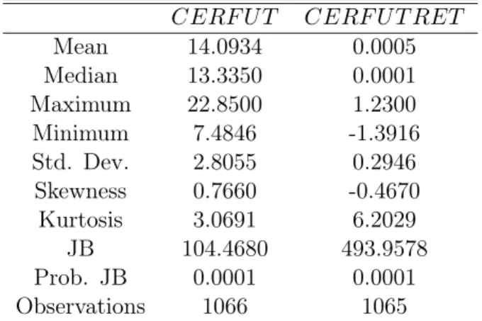
Table 2: Descriptive statistics for the CER ECX futures price CERF U T CERF U T RET
Mean 14.0934 0.0005 Median 13.3350 0.0001 Maximum 22.8500 1.2300 Minimum 7.4846 -1.3916 Std. Dev. 2.8055 0.2946 Skewness 0.7660 -0.4670 Kurtosis 3.0691 6.2029 JB 104.4680 493.9578 Prob. JB 0.0001 0.0001 Observations 1066 1065
Note: CERF U T stands for the EUA Futures Price, and CERF U T RET for the EUA Futures Price in Logreturn form. Std. Dev. is the standard deviation. JB stands for the Jarque Bera test.
Table 3: Estimation results of the two-regime Markov-switching VAR for EU AF U T RET and CERF U T RET
Log-likelihood 248.22
µ (Regime 1) 0.0021***
(0.0001)
µ (Regime 2) -0.0029***
(0.0001)
Equation for EU AF U T RET EU AF U T RET CERF U T RET
φ1 (Regime 1) -0.1088 0.1211** (0.0672) (0.0528) φ1 (Regime 2) 0.0895 0.1104 (0.0510) (0.0790) φ2 (Regime 1) 0.0994 -0.2105** (0.0551) (0.1149) φ2 (Regime 2) -0.1383* 0.1116 (0.0743) (0.0857)
Equation for CERF U T RET EU AF U T RET CERF U T RET
φ1 (Regime 1) -0.0869 0.1079 (0.0737) (0.0758) φ1 (Regime 2) 0.0661*** 0.0835** (0.0265) (0.0484) φ2 (Regime 1) 0.0704** -0.1230 (0.0340) (0.0963) φ2 (Regime 2) -0.0602*** -0.0838*** (0.0274) (0.0335)
Standard error (Regime 1) 0.0010 Standard error (Regime 2) 0.0007
Transition Probabilities Matrix Regime 1 Regime 2
Regime 1 0.9500*** 0.0700***
(0.0300) (0.0200)
Regime 2 0.0500*** 0.9300***
(0.0100) (0.0100)
Regime Properties Prob. Duration
Regime 1 59.37 19.05
Regime 2 40.63 14.05
Note: EU AF U T RET stands for the EUA Futures Price in Logreturn form. CERF U T RET stands for the CER Futures Price in Logreturn form.
Table 4: Robustness checks of the two-regime Markov-switching VAR for EU AF U T RET and CERF U T RET
Markov-switching VAR LR Statistic 26.758 p-value 0.001 Symmetry test 2.606 p-value 0.021 RCM 2-State 30.4526
Distributional Characteristics EU AF U T RET CERF U T RET
Mean 0.0006 0.0005 Median 0.0004 0.0002 Maximum 1.2120 1.1079 Minimum -2.2942 -1.1096 Std. Dev. 0.3459 0.2226 Skewness -0.4860 -0.4004 Kurtosis 6.3651 5.4188
Note: Distributional characteristics are given for the Markov-switching processes implied by the estimates in Table 3. EU AF U T RET stands for the EUA Futures Price in Logreturn form. CERF U T RET stands for the CER Futures Price in Logreturn form.