SEISMIC VELOCITY INVERSION USING MULTI-OBJECTIVE EVOLUTIONARY ALGORITHMS

HAL Id: tel-00120310

https://pastel.archives-ouvertes.fr/tel-00120310

Submitted on 14 Dec 2006

HAL is a multi-disciplinary open access archive for the deposit and dissemination of sci-entific research documents, whether they are pub-lished or not. The documents may come from teaching and research institutions in France or abroad, or from public or private research centers.

L’archive ouverte pluridisciplinaire HAL, est destinée au dépôt et à la diffusion de documents scientifiques de niveau recherche, publiés ou non, émanant des établissements d’enseignement et de recherche français ou étrangers, des laboratoires publics ou privés.

SEISMIC VELOCITY INVERSION USING

MULTI-OBJECTIVE EVOLUTIONARY

ALGORITHMS

Vijay Singh

To cite this version:

Vijay Singh. SEISMIC VELOCITY INVERSION USING MULTI-OBJECTIVE EVOLUTIONARY ALGORITHMS. Modeling and Simulation. École Nationale Supérieure des Mines de Paris, 2006. English. �tel-00120310�

______________ Collège doctoral

Ecole Doctorale n° 398 : "Géosciences et Ressources Naturelles"

N° attribué par la bibliothèque

|__|__|__|__|__|__|__|__|__|__|

T H E S E

pour obtenir le grade de

Docteur de l’Ecole des Mines de Paris

Spécialité "Dynamique et Ressources des Bassins Sédimentaires" présentée et soutenue publiquement par

Vijay Pratap SINGH

le 18 décembre 2006

APPLICATION DES ALGORITHMES ÉVOLUTIONNAIRES À LA DÉTERMINATION DE MODÈLES DE VITESSE

PAR INVERSION SISMIQUE

Jury

M. Bertrand DUQUET Examinateur

M. François JOUVE Examinateur

M. Gilles LAMBARÉ Rapporteur

M. Michel LÉGER Examinateur

M. Pascal PODVIN Examinateur

M. Marc SCHOENAUER Directeur

M. Médard THIRY Examinateur

APPLICATIONS DES ALGORITHMES ÉVOLUTIONNAIRES À LA DÉTERMINATION DE MODÈLES DE VITESSES PAR INVERSION SISMIQUE

RÉSUMÉ

Enjeux :

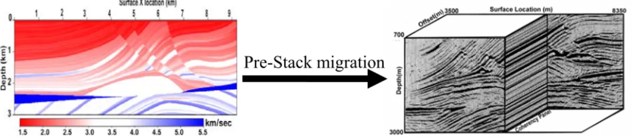
Le pétrole ne se manifeste à distance par aucune propriété physique permettant sa découverte. C'est pourquoi l'exploration pétrolière consiste à imager par la méthode sismique les pièges susceptibles d'en contenir. Le but de la migration, ou rétropropagation numérique des enregistrements sismiques, est de former une image des structures géologiques en replaçant en profondeur les réflecteurs qui ont causé les échos enregistrés. Les variations de la vitesse de propagation des ondes, de 1500 m/s dans l'eau à 6000 m/s et plus dans les roches sédimentaires compactes, rendent cette tâche critique car un modèle de vitesse erroné donne une image très distordue. Le coût énorme des forages effectués sur des structures fausses impose l'obtention d'images précises du sous-sol et donc la détermination du champ des vitesses sismiques, surtout en contexte de piémonts lorsque les images sont peu lisibles.

Positionnement du sujet :

Toutes les méthodes de détermination des vitesses exploitent la redondance des données sismiques : chaque portion de réflecteur renvoie plusieurs échos correspondant à des couples source-récepteur dont le déport, la distance de la source au récepteur, diffère. Certaines méthodes telles que la tomographie fonctionnent bien lorsque les structures géologiques sont assez simples pour que les réflexions soient bien reconnaissables sur l'ensemble des enregistrements, mais ce n'est pas le cas dans les piémonts. Nous avons donc choisi la migration itérative, dont le principe est que, la Terre étant unique, les images obtenues avec les différents déports doivent être superposables. Ce critère ne suffisant généralement pas à déterminer les vitesses correctes, il est nécessaire d'introduire des informations géologiques. Pour l'optimisation du champ des vitesses, les méthodes de gradient étant d'implémentation fort lourde, nous avons choisi un algorithme évolutionnaire pour sa simplicité, son adaptabilité, et surtout son automaticité. De plus, la diversité de la population optimale donne une idée de l'incertitude qui entache le résultat.

Résultats :

Parmi tous les champs de vitesses possibles, bien peu ont une géométrie géologiquement acceptables, d'où l'idée de ne manipuler que des modèles satisfaisant au critère de coupe équilibrée. Une coupe est équilibrée lorsqu'elle est compatible avec les hypothèses de conservation des épaisseurs et des longueurs mesurées le long des couches. Dans une première partie, nous avons montré que l'on pouvait non seulement générer des modèles géométriquement plausibles, mais aussi les optimiser relativement à des données de pendage de couches ou de position de chevauchements disponibles à l'affleurement ou dans des puits. La seconde partie concernant l'optimisation des vitesses n'a pu être reliée à la première. Dans cette seconde partie, nous avons représenté le champ de vitesses par des grilles. Par le choix d'un algorithme évolutionnaire multi objectif, nous avons pu faire coopérer efficacement les critères de semblance et de semblance différentielle qui, tous deux, mesurent l'invariance de l'image migrée quant au déport. Nous avons amélioré le réalisme des solutions en les lissant dans la direction du pendage. Enfin, nous avons extrait, des écarts à cette invariance, des corrections des grilles de vitesse qui accélèrent notablement la convergence. Les résultats obtenus sur les données Marmousi, un cas synthétique réaliste, sont satisfaisants. Sur les données réelles de Mer du Nord, le dôme de sel reste un problème non résolu par les méthodes automatiques, mais ses environs sont bien imagés.

Transfert des résultats vers l’industrie :

Le principal intérêt de la méthode développée est son automaticité et sa souplesse. Son créneau est le dégrossisage rapide de problèmes difficiles, avant qu'un interprétateur ne reprenne la main avec des méthodes interactives plus poussées, mais aussi plus exigeantes en expérience et plus consommatrices de temps humain.

Mots clés :

CHAPTER 1 ... 1

INTRODUCTION ... 1

1.1.MIGRATION VELOCITY ANALYSIS... 1

1.2.GLOBAL OPTIMISATION METHODS... 2

1.3.REPRESENTATION... 3

1.4.DOMAIN KNOWLEDGE... 3

1.5.THESIS OVERVIEW AND CONTRIBUTIONS... 4

1.6.SUMMARY OF CONTRIBUTIONS... 6

CHAPTER 2 ... 7

SURVEY OF EVOLUTIONARY ALGORITHMS (EAS) AND ... 7

MULTIOBJECTIVE EVOLUTIONARY ALGORITHMS (MOEAS) ... 7

2.1 INTRODUCTION... 7

2.2. EADEVELOPMENT HISTORY AND DISTINCTION BETWEEN EA’S... 9

2.3.1 Generational Evolutionary Algorithms... 9

2.3.2 Steady-State Evolutionary Algorithms ... 10

2.4.REPRESENTATION... 11

2.5.OPERATORS FOR THE REAL–VALUED EA ... 12

2.5.1 Crossover (or Recombination) operator ... 12

2.5.1.1. Discrete recombination (DR)... 13

2.5.1.2. Blend Crossover (BLX-α)... 13

2.5.1.3. Fuzzy recombination (FR) ... 14

2.5.1.4. Simulated Binary Crossover (SBX)... 15

2.5.2. Mutation... 16 2.5.2.1. Random mutation ... 16 2.5.2.2. Gaussian mutation ... 16 2.5.2.3. EXP mutation ... 17 2.5.2.4. Polynomial mutation ... 17 2.5.2.5. Non-uniform mutation... 17 2.6.SELECTION... 18 2.6.1. Proportional Selection... 18 2.6.2. Ranking selection... 19 2.6.3. Tournament selection ... 19 2.7. MULTIOBJECTIVE OPTIMIZATION... 21 2.7.1 Introduction ... 21

2.7.2. Multiobjective Optimisation Problem (MOP) ... 22

2.7.3. Pareto Concept ... 23

2.7.4. Pareto Dominance ... 24

2.7.5 Pareto Optimality... 24

2.7.5.1. Non-dominated set ... 24

2.7.5.2. Globally Pareto-optimal set... 25

2.7.5.3. Locally Pareto-optimal set... 25

2.7.6 Multiobjective optimisation approach ... 26

2.7.6.1. Aggregate fitness... 26

2.7.6.2. Pareto based ranking ... 26

2.7.6.3

ε

2.7.7 Overview of Multi-Objective Evolutionary algorithm (MOEA)... 28

2.7.7.1. Non-Pareto based approaches... 29

2.7.7.2. Pareto based approaches... 30

2.7.7.3 Nondominated Sorting Genetic Algorithm (NSGA) ... 31

2.7.7.4 Strength Pareto Evolutionary Algorithms (SPEA):... 32

2.7.7.5 Pareto Archived Evolutionary Strategy (PAES) ... 33

2.7.7.7 Non-Dominated Sorting Genetic Algorithm II (NSGA-II)... 36

2.7.7.8 Strength Pareto Evolutionary Algorithms 2 (SPEA2):... 38

2.7.7.10 Micro Genetic Algorithms... 43

CHAPTER 3 ... 45

VELOCITY MODEL DETERMINATION METHODS FOR COMPLEX SEISMIC DATA... 45

3.1INTRODUCTION... 45

3.2TIME DOMAIN METHODS... 46

3.2.1 Tomography methods... 46

3.2.2 Full waveform inversion methods ... 47

3.3. Depth domain methods... 48

3.3.1 Tomography migration velocity methods... 48

3.3.2 Image domain methods ... 50

3.3.2.1 Image perturbation criteria... 51

3.3.2.2 Differential Semblance Optimisation ... 53

3.3.3 Semblance function ... 55

3.4.KINEMATICS OF THE IMAGE IN OFFSET AND ANGLE DOMAIN... 57

3.4.1. Kinematics of the local–offset gathers for horizontal reflectors ... 57

3.4.2. Kinematics of the Angle gathers for horizontal reflectors ... 59

3.5MIGRATION... 59

3.5.1 Kirchhoff migration ... 60

3.5.2.DOWNWARD CONTINUATION METHODS... 62

3.5.2.1 Shot-profile migration (SPM) ... 63

3.5.2.2 Source-receiver migration ... 64

3.5.3 Comparison of Kirchhoff and wavefield-continuation method:... 65

CONCLUSIONS... 66

CHAPTER 4 ... 67

REPRESENTATIONS FOR EVOLUTIONARY MULTI-OBJECTIVE SUBSURFACE IDENTIFICATION... 67

4.1.INTRODUCTION... 67

4.2VORONOI-BASED REPRESENTATIONS... 69

4.3GEOLOGICAL KNOWLEDGE... 71

4.3.1 Geology... 72

4.3.2 Kinematic Models ... 72

4.3.3 The Contreras Model ... 73

4.4.THE EVOLUTIONARY ALGORITHM... 74

4.4.1 The Representation ... 74

4.4.2 Initialization and Variation Operators ... 75

4.4.2.1 Initialization... 76

4.4.2.2 Crossover Operator ... 76

4.4.2.3 Mutation Operator ... 77

4.4.2.4 The ε-Multiobjective Evolutionary Algorithm... 77

4.5FIRST RESULTS IN GEOLOGICAL MODELING... 78

4.5.1. The Geological Identification Problem... 78

4.5.2 The Evaluation Functions ... 78

4.5.3 A Three Fault Model... 79

4.5.4 Results on the Seven Fault Model ... 81

4.5.5 Convergence test... 83

4.5.6 Discussion on foothill identification ... 84

4.6 Velocity inversion of a foothill structure... 84

4.6.1 Two- step seismic velocity inversion ... 85

4.6.2 Single step seismic velocity inversion ... 87

... 94

CHAPTER 5 ... 94

INGREDIENTS OF MIGRATION VELOCITY ANALYSIS... 94

5.1INTRODUCTION... 94

5.2THE FITNESS FUNCTION... 95

5.2.1 Offset Domain Differential Semblance (ODS) ... 96

5.2.2 Modified Offset Domain Differential Semblance function ... 99

5.2.3 Angle Domain Differential Semblance (ADS)... 101

5.2.4 Modified Angle Domain Differential Semblance (MADS) ... 106

5.2.5DIFFERENTIAL SEMBLANCE OR SEMBLANCE ?BOTH! ... 108

AUTOMATIC GROSS VELOCITY ERROR ESTIMATION... 109

5.3INTRODUCTION OF RMO ... 109

5.3.1 RMO and Radon Transform... 110

5.3.2 Envelop ... 116

5.3.4 Results and Discussion... 117

5.4STRUCTURAL TRENDS AND DIP... 118

5.4.1 Sobel operator... 118

5.4.2 Example of Application... 120

5.5CONCLUSIONS... 122

CHAPTER 6 ... 123

SEISMIC VELOCITY INVERSION USING MULTI-OBJECTIVE EVOLUTIONARY ALGORITHMS... 123

6.1 Introduction ... 124

6.2 Multi-objective Evolutionary Algorithms... 126

6.3ε-MOEA FOR VELOCITY INVERSION... 129

6.4 Customized hybrid ε-MOEA for velocity inversion... 131

6.5. Main components of the customized ε-MOEA ... 134

6.5.1. Representation of velocity model ... 135

6.5.2. Objective functions... 135

6.5.3. Dip smoothing... 137

6.5.4. RMO correction ... 137

6.5.5. Synthesis of a parent ... 139

6.5.6. Reference Models... 141

6.6 Implementation of Customized Evolutionary Components ... 142

6.6.1 Initial Population ... 142

6.6.2. Guided crossover ... 146

6.6.2.1 Horizontal synthesis of Parent ... 146

6.6.3 Reference Models... 150

6.7. Results... 158

6.7.1. Evolutionary Algorithms and parameters ... 158

6.7.2. Marmousi Velocity Model... 161

6.7.2.1. 250m Grid sampling... 162

6.7.2.2. Superimposition of migrated image ... 170

6.7.2.3 100m Grid sampling... 171

6.7.3. L7 Model ... 175

6.8DISCUSSION AND CONCLUSION... 179

CHAPTER 7 ... 181

CONCLUSION AND PERSPECTIVE... 181

PERSPECTIVES... 182

Chapter 1

Introduction

To have significant geological information of earth requires an integration of different types of data and approaches. However one of the most successful approaches uses geophysical methods based on seismic data. Goal of seismic data processing is to convert a recorded wave field into a structural or lithological image of the subsurface. This requires a model of the wave propagation velocities of the subsurface. Nevertheless obtaining this model is often the most difficult processing step, in areas of complex structure such as foothill or salt body. The goal of this work is to develop an automatic seismic velocity estimation technique for such region using Migration Velocity Analysis (MVA) and global optimisation methods.

1.1. Migration Velocity Analysis

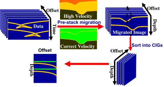
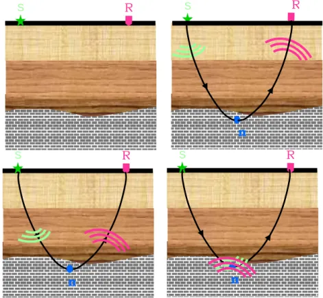
Most velocity estimation methods are based on the measurement of the kinematics of the reflections. An important difference among them lies in the way kinematics are measured, either directly from the data in the time domain, or after migration in the image domain. When geology structures are mild and lateral velocity variations are smooth, the kinematics measured on data space are usually robust and accurate. However in the presence of complex structure and/or strong lateral velocity variations, measurement of kinematic on the image space is more robust and accurate, even if migration velocity is

far from true velocity. Since migration focuses the energy, the incomplete focusing of reflection is a measurement of velocity error. Velocity estimation methods that use the focusing capability of migration to extract kinematics error are commonly known as Migration Velocity Analysis (MVA) methods.

MVA is an iterative process where each iteration is made of two distinct steps: (1) data are imaged by prestack migration and (2) the velocity function is updated based on the kinematics error measured on the migrated data. Due to the highly non-linear relationship between the velocity model and the focusing quality of image, velocity estimation is better solved when posed as optimisation problem. Both gradient and global optimisation methods have been used to estimate velocity. But because the objective function that is optimised during MVA is non-convex and has several local minima, the quality of initial velocity model is crucial for global convergence with gradient methods. On the other hand extreme computation cost is severe hindrance with global optimisation methods. The goal of this thesis is to develop a robust and efficient migration velocity estimation technique that uses global optimisation methods and remains computationally tractable.

1.2. Global optimisation methods

The objective of global optimization is to find the globally best solution of model, in the (possible or known) presence of multiple local optima. Since velocity optimisation problems in geologically complex regions are non-linear, non-convex and ambiguous, we have chosen Evolutionary Algorithms (EAs) for optimisation. EAs are stochastic search methods that mimic the metaphor of natural biological evolution. EAs operate on a population of potential solutions, applying the principles of blind variation plus survival of the fittest to produce hopefully better and better solutions.

Generic EAs have to search a large parameter space with a little exploitation of domain-specific information from previous iteration to find global optimal solutions. Consequently they are usually computationally expensive and/or have to give up on

precision. In this thesis attempts have been made to reduce the computational cost of EA by adding geological and geophysical knowledge to the component of the algorithms, at the representation level, in the variation operators and in the objective function.

1.3. Representation

Acute computation demand of global methods imposed to a concise representation of velocity model. A lot of attempts have been made for representations e.g. B-spline, Bi-cubic, horizontal layers, and Voronoi representation. It has been noticed that some representations are very concise, however unable to represent a real geological structure, whereas other which are geologically significant require a large number of parameters. Therefore in this thesis we made an attempt to represent a velocity model for foothill structure that is concise as well as geologically significant.

In this work, after some effort to design a concise and geologically meaningful representation, we finally concluded that the grid representation was the most flexible one, even though it implies a large number of unknown parameter and induces a high computational cost. Hence we started to look for domain specific ways to reduce the computational cost.

1.4. Domain Knowledge

Traditional methods extract a lot of information about the velocity model from the geological knowledge and the migrated data to correct the velocity model, as for example the geological knowledge that “generally velocity increase with depth, varition of velocity along layer is small” and “salt body have almost fix velocity”. A lot of information about the velocity can also be extrated from the gathers using residual move out (RMO) curves. They also provide information about global as well as local goodness of a velocity model. Hence we decided to use these information in our approach and have therefore developed domain specific operators. The result is a customised hybrid algorithms.

1.5. Thesis overview and contributions

Review of EAs and MOEAs: Because we made the choice of EAs as optimisation

methods we started by giving in chapter 2, an overview of Evolutionary Algorithms. First, concepts and development of evolutionary algorithms along with different components of EAs (crossover, mutation, and selection) are described. Multiobjective optimisation and related concept are then introduced and state-of-art MultiObjective Evolutionary Algorithms (MOEAs) are surveyed.

State of art in velocity optimisation tools: In chapter 3, we review the state of the art of

seismic velocity estimation techniques. We discuss time domain techniques i.e. tomography and waveform inversion, depth domain techniques i.e. tomography migration velocity analysis, and fully automatic techniques based on Differential Semblance Optimisation (DSO).

Representation: In chapter 4, we present a cross-section balancing representation for

foothills (Singh et al. 2005a and 2005b). The goal is to represent a subsurface structure in a geologically sound manner, thus obtaining a concise representation of velocity models. We successfully apply this representation to the seismic velocity inversion with optimised geological structure (Singh et al. 2005). However the limited success of a first attempt to simultaneously invert both geological and geophysical criteria leads to go back to grid representation. At this point, looking for an optimal grid size, some experiments on different grid sampling demonstrate that a too coarse sampling may lead to ambiguity.

Ingredients of velocity inversion: In Chapter 5, we modify the Differential Semblance

function (Symes, 1991) in both offset and angle domains. Modified differential semblance functions are “more convex” than the original one, and less sensitive to migration parameter settings, even for large velocity errors (Singh et al. 2005) (we shall use those modified differential semblance function and semblance function simultaneously to optimize velocity model in Chapter 6). We also present an automatic

Residual MoveOuts (RMO) extraction technique from gathers to estimate the approximate velocity error (that will be used in Chapter 6 for correcting the velocity error of the models during their optimization). Structural trends of the geological model provide significant information about the velocity model. Here we extract this information and use it reduce the velocity variation along the layers.

Automatic seismic velocity estimation using MOEA: In Chapter 6, we present our

main realization, the algorithm for automatic seismic velocity inversion, and some results obtained on both two problems. This velocity analysis method inherits the characteristics of wavefield extrapolation, mainly robustness in presence of large and sharp velocity contrast, as well as its ability to cope with multipathing. Since a global optimisation method is used, we are free from linearization of the wave equation. The basis of our algorithm is a Multi-Objective Evolutinoary Algorithm, but, in order to increase its efficiency, we first customize the algorithm itself, and also propose a new exploitation operator. The goal of the customization is to strive to have both the robustness of global methods and the efficiency of local optimisation methods. We present examples of migration velocity analyses mainly on Marmousi model, together with a few results on the North-Sea L7 model. We demonstrate that our automatic velocity analysis technique is able to cope with large velocity error and is as efficient as the gradient methods except in salt body.

Conclusions and Perspective: In Chapter 7, we conclude our research and discuss about

the possible 3D extension of our approach. Also, there is a need for adding human information during the optimisation, and integrating with some other linearized approach (Save and Biondi, 2004; Shen et al., 2004) to get a precise model. For 3D extension one may require to smartly and efficiently use migration algorithms, exploit the information from migrated data for further improvement and generation of models.

1.6. Summary of Contributions

In this thesis our first contribution is the development of an automatic cross-section balancing algorithm for foothill structure (Chapter 4). It can be generalized to other structures. We made an effort to analyze the influence of different type of representations (i.e. Voronoi, geological, and grid). We notice that representation is mostly geologically dependent and that the number of parameter is not the main issue when choosing a representation. Our second and major contribution is the development of an automatic tool for seismic velocity estimation, using a customized MOEA, and domain-specific operator where we have introduced domain knowledge. Using such tool, we were able to solve model with a large number of unknown parameters at a reasonable computation cost.

Chapter 2

Survey of Evolutionary Algorithms (EAs) and

Multiobjective Evolutionary Algorithms (MOEAs)

2.1 Introduction

The buzzword doing the beats at all hierarchical levels of the industry today is optimisation. Calculus had been the reigning emperor of optimisation techniques until recently, when global optimisation techniques have been put to use. Among those various techniques, one of the most promising is Evolutionary Computing (EC), which mimics the natural process of evolution. It is based on Charles Darwin’s theory of evolution, where nature selects the best genetic settings to survive in the next generation and some random change may occur during next generation birth. Evolutionary algorithm similarly selects the best performing solutions from the current population, and uses the variation operators of crossover and mutation to generate further solutions. An important feature of biological evolution is robustness - which is what evolutionary algorithm (EA) strives to achieve.

Essentially, EAs are a method of “breeding” solutions of a optimisation problem by means of simulating evolution. Since it is inspired by the natural selection and genetics, evolutionary computation borrows much of its dialect from genetics, cellular biology and evolutionary theory. In EC, a candidate solution is known as an individual. The collection

of current individual in the system is collectively known as the population. The actual encoding of an individual’s solution is known as its genome (or chromosome) and representation is known as genotype. The way solution operates when tested in the problem environment is known as the individual’s phenotype. When the individuals are modified to produce new individuals, they are said to be breeding. After the evaluation, a individual gets a mark, known as its fitness, which indicate how good a solution it is. The period of evaluation and assignment of fitness to a individual is known as fitness

assessment. The whole process of finding an optimal solution is known as evolving a solution.

50‘s and 60‘s

The Michigan The German The California

(Holland) (Rechenberg, Schwefel, Bienert) (Fogel, Owens, Walsh)

- More emphasis on recombination,

inversion, etc. - Used the term

“genetics”

- More emphasis on selection and mutation - Used the term “evolution”

evolution strategies simulated evolution

Evolution

Strategies

Evolutionary

Programming

Genetic

Algorithms

+

Programming

Genetic

put to automatedprogramming

t

o

d

a

y

2.2. EA Development history and distinction between EA’s

Historically, four evolutionary computation paradigms have emerged. They are: (i) evolution strategies, (ii) evolutionary programming, (iii) genetic algorithms, and (iv) genetic programming. Though during the last few years, these paradigms have crossbred and their lines of distinction have blurred, each of them had different features (Figure 2.1). The main difference between these evolutionary algorithms lies in their representation and genetic operators (Bäck, 1996). The operators are closely related with the underlying representation scheme of each evolutionary algorithm.

Genetic algorithms typically work on fixed-size bit-strings using crossover as its main operator. Evolution strategies are based on vectors of real values for representation and use mutation as the main operator. Evolutionary programming usually manipulates graphs using mutation as the single genetic operator. Genetic programming represents individuals as trees of flexible size. Another difference lies in the way selection is applied: GA use propositional selection and generational replacement, though rank based selection has become more popular over the years. Evolutionary strategies use deterministic replacement and no parent selection while evolutionary programming uses tournament replacement.

From now onward we will not detail all possible variation of EAs (see instance Eilven and Smith, 2003) but only the ones that are uses within Multi-objective EAs. There are two common high level, conceptual procedures made use of in evolutionary computation. The first one is the traditionally used generational EA, whereas the second approach is steady-state EA which is progressively a more popular newcomer.

2.3.1 Generational Evolutionary Algorithms

First, a set of random individuals (models) is generated. Then, each individual in the initial population is evaluated and fitness is assigned to them. The better individuals from the members of an initial or old population are selected for breeding and form a new population. This new population is evaluated and then mixed with the already existing

old population. An altogether optimal new population is created from this assembly (old + new population). This process is continued until an ideal individual is discovered or resources are exhausted. The pseudo code of the generational Evolutionary is as follows:

Algorithms : Generational Evolutionary Algorithm Begin EA;

t = 0; // Initializing time

Random P(t); // Initialize a usually random population of individuals: Evaluate P(t); // Evaluate the fitness of all individuals

While not done do // Testing for termination criterion t = t + 1; // Increasing time

P’’ = select P(t); // Select a sub-population for offspring production Recombine P’’(t); // Recombine the “genes” of selected parents

Mutate P’’(t); // Stochastically perturb genes of the mated population: Evaluate P’’(t); // Evaluate the new fitness

P = survive P(t), P’’(t) // Select the survivors from actual fitness: End while;

End EA;

2.3.2 Steady-State Evolutionary Algorithms

In contrast to the generational EA, where a whole offspring population is created in every generation, in steady state EA only one or a few individuals are created and immediately integrated back into the parent population in each generation. The term steady-state means that in one step only a small change takes place without the whole population changing. The pseudo code of the steady-state EA is given below

Algorithms: Steady-state Evolutionary Algorithm Begin EA;

t = 0; // Initializing time

Random P(t); // Initialize a usually random population of individuals Evaluate P(t); // Evaluate the fitness of all individuals

While not done do // Testing for termination criterion t = t + 1; // Increasing time

P’’i = select P(t); // Select a few parents for offspring production:

Recombine Pi’’(t); // Recombine the “genes” of a few selected parents

Mutate Pi’’(t); // Stochastically perturb genes of the mated parents

Evaluate Pi’’(t); // Evaluate the new fitness of offspring

P = survive P(t), Pi’’(t) // Select the survivors from actual fitness:

End while; End EA;

Of course the practical meaning of the word “generation” is fairly different in both cases: important population modification for generational evolutionary algorithms, modification of a few individual in for steady state evolutionary algorithms.

2.4. Representation

The choice of representation is one of the most critical point of the design of any EA, since it will likely have a strong impact on the algorithm’s overall performance. The EA design decision should be parsimonious in defining the representation, to limit the size of search space and to avoid generating potentially infeasible solutions. The design should be based on the physics of the problem and it should also be constrained by the domain knowledge. To avoid the generation of infeasible solutions, each parameter should be constrained by the feasible range. In Chapter 4 few geological representation techniques and related issues are described.

Once the model is chosen, then might be different way to encode it (i.e. binary, real, integer, finite state automata). For a given problem, certain encoding (or encodings) may result in a relative compact search space, which is beneficial. For example binary encoding for discrete search space, real encoding for real valued parameters are most favorable. Similarly, structural encoding, such as grammatical encoding, is one of the most efficient ways to represent network topologies.

Our discussions about the EA operators are w.r.t real value. The various operators of the real–value EAs are briefly described in the following section.

2.5. Operators for the real–valued EA

In real-coded EA, parameter, considered as genes, are used directly to form a genotype. The use of real–valued EAs for real function optimisation facilitates the problem of coding and decoding genotypes and phenotypes. A genotype represents a solution, and population is a collection of such solutions. The operators (selection, recombination and mutation) modify the population of the solutions of any representation to create a new (and hopefully better) population. The various cross-over and mutation operators are briefly explained in the following subsections.

2.5.1 Crossover (or Recombination) operator

The recombination operator combines the genes of two or more parents to generate better offspring. The main purpose of a crossover operator is to recombine the partial good information from two or more parents so as to generate better offspring. Crossover occurs during evolution according to a user-definable crossover probability. The crossover plays a central role in EAs, in fact it may be considered as one of the algorithms defining characteristics. It is one of the components to be borne in mind to improve the behaviors of EAs (Liepins et al., 1992).

In real parameter EA, the main challenge is how to use the real parameter vectors to create a new pair of offspring vectors. In what follows, a real parameter crossover is

described followed by few real-parameter mutation operators. A good overview of many real parameter crossover and mutation operators can be found in Herrara et al. (1998)

2.5.1.1. Discrete recombination (DR)

DR corresponds to a standard uniform crossover in the binary case. Geometrically it is represented in Figure 2.2. Only cross sites are allowed to be chosen at the variable boundaries (green point). The offspring O1i∈(P1i, P2i) for each 1≤i≤n. This crossover operator

does not have adequate search power because the set of the possible values for each parameter is unchanged. Therefore we need mutation operator to change the set of possible values.

Figure 2.2: Discrete recombination on two decision variables. Parents are represented

in pink and offspring are represented in green. This operator does not have adequate search power.

2.5.1.2. Blend Crossover (BLX-α)

The BLX cross-over was proposed by Eshelman and Schaffer (1993). For the ith parameter, and two parents Pt1i and Pt2i the blend recombination (BLX- α) creates at each

generation t one offspring Ot+1i that can be represented as follow:

Ot+1i = Pt1i + β (Pt2i - Pt1i ),

where β is a random variable in the interval [-α , 1+ α]. The value α defines the size of area for possible offspring (Figure 2.3). If α value is more than 0 than it add exploration property whereas α =0 adds the exploitation property. If α is set to zero, this recombination creates a solution inside the range defined by the parents (see Figure 2.3) given area. It is also called arithmetic by Michalewig and intermediate by Rechenberg and Schwafel. P1i P2i O1i O2i P1 P2

Figure 2.3: The BLX- α operator. Parents are represented in pink, offspring in green and

upper and lower limit in rose colour. BLX-a uniformly picks new individuals with values that lie in [P1i- α I, P2i+ α I].

If the distance between the parents solution is small, the difference between the offspring and parents solution is also small. This property makes the search operator partially adaptive.

2.5.1.3. Fuzzy recombination (FR)

Fuzzy recombination operator was proposed by Voigt et al. (1995). The probability that the offspring has the value Oi is given by a bimodal distribution

p(Oi)∈ (φ(P1i), φ(P2i) )

With triangular probability distribution ψ(r) having the modal values P1i and P2i with

P1i – d.| P2i - P1i | ≤ r ≤ P1i +d. | P2i - P1i |

P2i –d.| P2i - P1i |≤ r≤ P2i +d.| P2i - P1i |

for P1i ≤ P2i and d ≥1/2. Geometrically, it is represented in Figure 2.4

Figure 2.4: The FR operator, parents are in pink colour and offspring in green, lower

and upper limits in rose colour. Each triangle denotes the probability of the offspring to resemble each of its two parents.

PiL Oi P1i P1i PiU

d

PiL P2it_Oit+1 P1it_O PiU it+1

I

This operator gives importance to the creation of a solution near to its parents. The distribution can be changed with the parameter d. If d is large the solution will be away from the parents and vice versa.

2.5.1.4. Simulated Binary Crossover (SBX)

Simulated binary crossover (SBX) operator for real variables was first introduced by Deb and Agrawal (1995). This operator gives similar results to those that would be given if the parents were binary encoded, and binary single crossover were to be performed. This operator respects the interval schemata processing, in the sense that common interval schemata of the parents are preserved in the offspring’s. The SBX crossover puts the stress on generating offspring in proximity to the parents. So, the crossover guaranties that the range of the children is proportional to the range of the parents, and also favors that near parent individuals are more likely to be chosen as children than individuals distant from the parents. These crossovers are self-adaptive in the sense that the spread of the possible offspring solutions depends on the distance between the parents, which decreases as the population converges.

The procedure of computing offspring P1i t+1 and P2i t+1 from the parent solutions P1i t

and P2i t is as follows. First, a random number ui is generated between 0 and 1, thereafter

a spread factor βi = | P2i t+1 - P1i t+1 | / | P2i t - P1i t | iscalculated using specified probability

distribution function given below. These probability distribution functions are used to create an offspring using the following relation (Deb and Agrawal, 1995):

P(βi) = 0.5 (ηc+1) βiηc , if βi ≤ 1 ;

P(βi) = 0.5 (ηc+1) / βiηc , otherwise.

ηc (distribution index) is a non-negative real number. βi is calculated by equating area

under the curve equal to ui using the following relation.

βi = (2ui )1/ηc +1 if ui ≤ 0.5 ;

βi = (1/2(1-ui ))1/ηc +1 otherwise .

After getting the βi from the above relation the offspring is calculated as follows

xi (2, t+1) = 0.5 [ (1 - βi ) xi (1, t) + (1 + βi ) xi (2, t) ] .

A large value of ηc gives a higher probability to generate 'near parent' offspring (Figure

2.6).

Figure 2.6: A large value of ηc has a higher probability to generate offspring similar to the

parents and vice versa (Deb and Agrawal, 1995).

2.5.2. Mutation

Mutation provides a mechanism for maintaining diversity in a population. In one way, it acts as a safeguard against premature convergence by randomly changing the value of one or more allele in a chromosome. However, for real-coded genetic algorithms, it often plays the main role. Several mutation types are in use and we describe below few widely used ones.

2.5.2.1. Random mutation

Each variable that is going to be mutated is assigned a value, laying within its feasibility range (see Michalewicz, 1992).

2.5.2.2. Gaussian mutation

This mutation is similar to the previous one, except that the mutation step ∆Pi is calculated according to a Gaussian’ distribution. Smaller mutation steps are much more probable then large mutation steps. This is the standard in evolutionary strategies

(Rechenberg 1973, Schwefel 1977, Bäck 1995a). Oit+1 = ri (PiU - PiL) where ri is a random

number between [0,1].

2.5.2.3. EXP mutation

This mutation type comes from the idea that the role of mutation at the beginning is to make larger jumps, whereas later on, as the search progresses, fine tuning is achieved by making smaller jumps.

2.5.2.4. Polynomial mutation

Polynomial mutation was proposed by Deb and Goyal (1995). If x is the value of the ii th

parameter selected for mutation with a probability pm and the result of the mutation is the

new value yi _{obtained by a polynomial probability distribution}

( )

(

)

(

)

x are the lower and upper bound of x respectively i

and r is a random number in [0,1] i i L i U i i i x x x y = +( − )δ

The distribution is controlled by the parameter ηm_{(distribution index).}

2.5.2.5. Non-uniform mutation

Non-uniform mutation was first introduced Michalewicz (1992). According to this, the probability to have the value y after mutation for the ith parameter is

(

)

if r

<0.5

if r

≥

0.5

(

)

where tmax _{is the maximum number of generations, b a user is specified control}

parameter and τ a random bit, 0 or 1. The exponent ofr approaches 0 as t approaches i

tmax andy is closer toi x . This allows reducing the search closer to the optimum value as i

the evolution proceeds.

2.6. Selection

An evolutionary algorithm performs a selection process in which the best fitting members of the population survive, whereas, the “least fit” members are eliminated. In a constrained optimization problem, the notion of “fitness” partly depends on whether a solution is feasible (i.e. whether it satisfies all the constraints), and partly on its objective function value. Selection provides the driving force in an evolutionary algorithm and the selection pressure is a critical parameter. If the selection pressure is too high the search will terminate prematurely, and if the pressure is too low progress will be slower than necessary. There exists a variety of selection algorithms: Goldberg and Deb (1991) performed some analysis on some of the most commone algorithms used in Genetic Algorithms (GAs).

2.6.1. Proportional Selection

In proportional selection, the individuals are selected according to their relative fitness values. The selection probability of ith individual Iig at generation is defined as

P(Iig ) = f(Iig ) /Σλi=1 f(Iig ).

This is a probabilistic selection method in which every individual having non-zero fitness will have a chance to be reproduced. This selection scheme is adopted by the simple genetic algorithm and believed to be the most similar mechanism that occurs in nature. One problem with the fitness-proportional selection is that it is directly based on the fitness. Assessed fitness is rarely an accurate measure of how “good” an individual really is.

2.6.2. Ranking selection

Ranking selection is a selection method which assigns selection probabilities solely on the basis of the rank i of individuals, ignoring absolute fitness values. In (µ, ) uniform ranking (Schwefel, 1995), the best µ individuals are assigned a selection probability of 1/ µ while the rest are discarded:

1/ µ 0≤i≤ µ P(Iig ) = 0 µ≤i≤λ

2.6.3. Tournament selection

This is the most popular selection mechanism. It is popular because of it is simple, fast and has well understood statistical properties. Tournament selection (Blickle and Thiele, 1995) is performed by choosing parents randomly and reproducing the best individual from this group. When the number of parents is q, this is called the q-tournament selection. The standard values of q are 2 and 7. Value 2 is used in GA whereas 7 is used in GP. Value 2 is weakly selective whereas value 7 is highly selective.

There are many other types of crossover operator like unimodal normally distributed crossover (UNDX) (Ono and Kobayashi, 1997), simplex crossover (Tsutsui et al., 1999), fuzzy connective based crossover (Herrara et al., 1995) and uniform average crossover (Nomura and Miyoshi, 1996). The comparisons of these crossover operators are mainly context dependent. The issue of exploration and exploitation make a crossover dependent on a chosen selection operator. Beyer and Deb (2001) argued that in most situations selection operator reduces the diversity. The reduction of diversity due to the selection operator can be related to the exploitation property of selection operator. Hence, in general, crossover operator should enhance the population diversity. Such a balance between the descent and ascent of diversity will allow EA to have an adequate search property (Figure 2.5) Based on this argument; two postulates have been recently suggested by Beyer and Deb (2001).

First population mean should be invariant before and after the crossover. Second population diversity may increase after the crossover.

Figure 2.5: When selection is reducing the diversity, the variation should increase the

diversity. Balancing the two allows EAs to have adequate search property.

Since real parameter crossover operator directly manipulates two or more real number to create one or more number as an offspring, one may wonder if there is a special need for using another mutation operator. The confusion arises because both operators seem to perform the same task, i.e. perturb every solution in the parent population to create a new population. The distinction among various operators lies in the extent of perturbation allowed in each operator. Although it is highly debated in literature, Deb (2000) believed that distinction between these two lies in the number of parent’s solution used for perturbation process. If only one parent is used for perturbation then it is called mutation On the other hand, if more than one parents are involved for perturbation then it is called crossover.

2.7. Multiobjective

optimization

2.7.1 Introduction

Multiobjective optimisation is different from single-objective optimization in that it involves consideration of more than one, and often conflicting, objective functions. Many real world design problems involve multiple, usually conflicting optimization criteria. Often, it is very difficult to weigh the criteria to build a global criterion. Multiobjective evolutionary algorithms use the principle of Pareto optimality, which states that, a model is “Pareto optimal” if it is not possible to improve it with respect to any criterion without worsening it with respect to at least one other criterion. This in turn allows the user to choose among many alternatives.

Figure 2.6: Ideal Multiobjective Optimisation and traditional preference based

optimisation. Traditional preference based methods require multiple run and need to define weight for obtaining trade of solution, whereas ideal multiobjective optimisation gives possible trade of solution in a single run.

Multiple trade-off solutions f2 f1 Higher level of information Multiobjective optimisation problem mininize f1 minize f2 ... minize fn Subjective to constrain Ideal Multi-objective optimiser Higher level of Information Estimate a relative importance vector (w1 +w2 +w3 +…)

Single objective optimisation

F= (F1w1 +F2w2 +F3w3 +)

Single objective optimiser Preference Based Approach

Multiobjective is not only different in terms of number of objective function but also in term of number of search spaces. Single objective optimisation has only parameter search space, whereas multiobjective optimisation has two search space parameter and objective space (Figure 2.7). As a result multi-objective optimizations produce a number of compromise solutions, known as the Pareto-optimal solutions. It is not a consequenc of algorithms, it is a choice. The task in a multi-objective optimization problem is to find as many Pareto-optimal solutions as possible. Classical optimization methods are not efficient in finding multiple Pareto-optimal solutions. The major difficulty with all classical methods is that they require multiple run and need to define weight to each objective to obtain multiple Pareto-optimal solutions (Figure 2.6) and they sometime can not find whole front (concave front).

Evolutionary algorithms (EAs) are ideally suited to solve multi-objective optimization problems, simply because multiple Pareto-optimal solutions can be captured in a single population by suitably modifying the EA selection operators. Additionally, evolutionary algorithms are less sensitivity to the shape or continuity of the Pareto front (Coello, 2001).

With multiobjective optimization problems, knowledge about the Pareto-optimal set helps the decision maker in choosing the best compromise solution. For instance, when simulating a mountain front, a geologist works on an existing model space exploring multiple model possibilities to arrive at the best possible model. Thereby, the model space is reduced to a set of optimal trade-offs. However, generating the Pareto-optimal set is computationally expensive and often infeasible, because of the complexity of the underlying application, which prevents exact methods from being applicable. EAs also do not guarantee the identification of optimal trade-offs but try to find a set of solutions that are (hopefully) not too far away from the optimal front (Figure 2.6).

2.7.2. Multiobjective Optimisation Problem (MOP)

A multiobjective problem (MOP), also called criteria optimization, or multi-performance or vector optimization involves a vector of N parameter x _{, a vector of M}

objective functions, and a vector of L dimensional constraint gl x . The objective

function as well as constrains are functions of the parameter. Since minimizing Fm( x ) is

equivalent to maximizing - Fm( x ), we may assume minimization in all cases without

any loss of generality.

Minimizing Fm(xr)=(f1(xr),f2(xr),...fm(xr)) _{m=1, 2...M;}

subjected to gl x g1 x , g2 x , .. .. . .. gl x 0) l= 1,2…L;

where x x1, x2, .. . .. .. . xn xi L

x_i x_iU _{i= 1,2,…..N}

Each parameter xi has to take a value within a lower bound xi L

and an upper bound xi

U

. If any solution x _{satisfies all the L constraint} gl x and all the 2N variable bounds, it is called as a feasible solution, and infeasible in other cases. In the presence of constraints, the entire parameter space need not be feasible.

Figure 2.7: Representation of parameter space and corresponding objective space.

2.7.3. Pareto Concept

The concept of Pareto-optimum was first introduced by Vilfredo Pareto (Pareto 1886). The key Pareto concepts for the minimization problem are defined as follows:

a x2 x3 x1 f₁ f2 Parameter Space Objective Space

2.7.4. Pareto Dominance

For any two decision vector ar=(a1,a2,...an)_and b =(b1,b2,...bn)

r , b ar < r (ar dominatesbr) if F_m

( )

( )

F

(

a

)

F

(

b

)

r

r ≤

F

(

a

)

F

(

b

)

F

(

b

)

F

(

a

r

)

r

r

r

_≠

_∧

_≠

Based on the Pareto dominance concept in a multi-objective problem, a solution for which there is no way of improving any-objective without worsening at least one other objective is called a Pareto-optimal solution. A graphical representation of Pereto optimal (non-dominated) and dominated solutions is depicted in Figure 2.8.

Figure 2.8: Representation of Pareto optimal solutions and dominated solution. Blue

front is the final Pareto optimal solution, whereas green and pink fronts were Pareto optimal at particular instant. Now they are dominated by Blue front solution.

2.7.5 Pareto Optimality

2.7.5.1. Non-dominated set

Among a set of solutions S, the subset of non-dominated solutions S’ are those that are not dominated by any member of S. In Fig. 2.8, blue dots represent the non dominated solutions and they are called Pareto-optimal solutions. Fig. 2.9 shows the Pareto-optimal sets for different possible combinations of maximization and minimization functions.

Pareto optimal = non-dominated

F1 F2

2.7.5.2. Globally Pareto-optimal set

The non-dominated set of the entire feasible search space S is the globally Pareto-optimal set.

2.7.5.3. Locally Pareto-optimal set

If for every member x in a set P, there exists no solution y (in the neighborhood of x such that ⎜⎜y-x⎜⎜∞ ≤ε , where ε is a small positive number) dominating any member of the set P, then the solutions belonging to the set P constitute a locally Pareto-optimal set (Miettinen, 1990 ; Deb, 1999c).

Figure 2.9: Representation of Pareto front shape in different Min –Max condition of

objective function.

f

f

f1

f2

2.7.6 Multiobjective optimisation approach

To solve multiobjective problem with EA, the only things that need to be modified is the selection. In multiple-objective fitness assessment, an individual receives separate assessments in each of the criteria of interest, and the system must determine how to select individuals based on some function of these criteria. There are two common strategies for doing this, aggregate fitness and Pareto ranking. Now a day a recently developed approach based on ε-dominance concept is routinely used. Here we present aggregate fitness, Pareto ranking and ε-dominance based strategy for selection.

2.7.6.1. Aggregate fitness

Here the strategy is to join each individual’s assessments into single aggregates fitness by which the individual is selected. The most straightforward aggregation approach is simply to add the various assessments as a weighted sum (Hajela and Lin 1992). An alternative way to do this is to set the standardized fitness to the maximum (worst) of the various fitness assessments (Wilson and Macleod 1993). A third aggregation technique known as lexicographic ordering is used with ranking and tournament selections (Fourman, 1985). Lexicographic ordering assumes that there is an order of importance among the criteria. Here, individuals are first sorted (for ranking or tournaments) by the most important criterion. Ties are then broken by ranking by the second criterion, then the third criterion, etc.

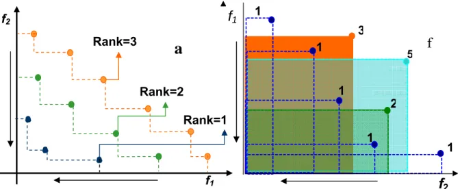
2.7.6.2. Pareto based ranking

In this set of method, individuals are ranked according to some Pareto based mechanism. There are two common techniques which result in Pareto ranking. The first technique, by Goldberg (1989), consists in assigning rank “1” to all the individuals who are not dominated rank ‘”2” to nondominated remaining individuals and so on. This ranks individuals in layers based on their domination of others (Figure 2.10a). The second technique by Fonseca and Flemming (1993) simply sets an individual’s standardized fitness as the number of individuals in the population which dominate that individual

The Pareto ranking procedures based on the above two procedures are summarized in Table 2.1.

Figure 2.10: Pereto ranking according to Goldberg’s (1989) at left and according to

Fonseca and Fleming (1993) at right.

Table: Steps of Pareto ranking for Goldberg’s (1989) and Fonseca and Fleming (1993). procedure:

Goldberg’s method (1989)

procedure:

Fonseca and Fleming method (1993)

input: individual fk, k=1, 2, …, popSize

output: fitness eval(fk)

step 1: rank 1 is given to the nondominated individuals

step 2: removing them from contention. step 3: finding the next nondominated individual, removing them from contention, rank 2 is assigned to them.

step 4: process continues until the entire population is ranked, and

output fitness eval(fk).

input: individual fk, k=1, 2, …, popSize

output: fitness eval(fk)

step 1: rank 1 is given to the nondominated individual

step 2: removing them from contention. step3: finding the next nondominated individual, removing them from contention, rank equally to the number of its dominating individuals plus one.

step 4: process continues until the entire population is ranked, and

output fitness eval(fk).

f

a

f

f

2.7.6.3

ε

-dominance ranking

The ε-dominance sorting is done in two steps: (1) sorting of non-dominance solutions (2) ε-box (εi*fi , where fi min is the minimum possible value of the ith objective and εi is the

allowable tolerance in the ith objective, below which the values are insignificant for the user.) is created for each solution and after that ε non-dominance box solutions are sorted. This approach maintains the diversity along the Pareto front and help in fats convergence. The concept of ε-dominance is illustrated (Figure 2.11).

Figure 2.11: Illustration of ε-dominance concept.(a) dominance solution (b) the ε

-dominant solution by star and ε-dominant region by background colour (c) After sorting

ε-dominant solution.

2.7.7 Overview of Multi-Objective Evolutionary algorithm (MOEA)

Multi-objective problems (MOP) were first discussed by Rosenberg in 1967. The first reported implementation and test of a multi-objective evolutionary approach was the Vector Evaluated Genetic Algorithm (VEGA) by Schaffer (1984). Since this branch of EA has attracted many researchers dealing with non-linear, non-convex and integer-variable multi-objective optimization problems.

Recently, there has been a surge in research on new, and particularly genetic/ evolutionary multi-objective optimization algorithms and their applicability to various optimization problems (Coello, 2001; Corne et al., 2000; Deb et al., 2002; Jensen, 2003; Knowles and Corne, 2000; Tan et al., 2002; Zitzler and Thiele, 1999). Fonseca and Flemming (1993) classified the MOEA into three groups, namely: (i) plain aggregation

f1 f2 f1 f2 f1 f2

a

_b

_c

approaches used to handle the MOP are Non-Pareto and Pareto based approaches. The evolution of MOEA is shown in Figure 2.12

Figure 2.12: Key developments of multi-objective evolutionary algorithms.

2.7.7.1. Non-Pareto based approaches

The Vector Evaluated Genetic Algorithm (VEGA; Schaffer, 1985) is a non-Pareto based approach. It is a straight forward extension of single objective GA. In each generation, GA population is randomly divided into subpopulations, equal to the number of

Epsilon-dominance

Laumanns, Thiele, Deb and Zizler (2002)

Pareto-based MOEAs

MOGA, NPGA , NSGA, (1993-1995)

Development History of Multi-Objective

Evolutionary Algorithms

Penalty -Based approach

Non Pareto-based

ESVO[Kursawe 91]

Goldberg's Suggestion (1989)

Pareto-based selection and

niching mechanisms

Elitist MOEAs

SPEA, SPEA2, MOGAs, PAES, NSGA-II , etc. (1998 - Present)

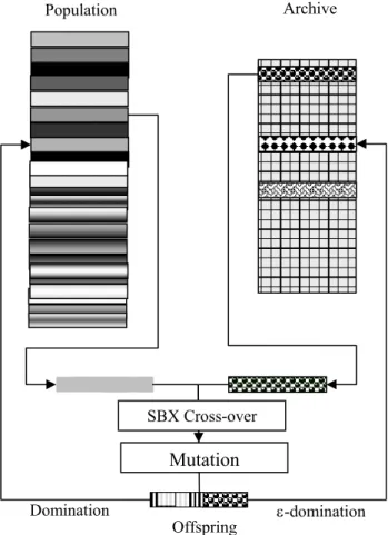
Epsilon-MOEA (2003)

objectives. Each subpopulation is assigned a fitness based on different objective functions. In this way, each objective function is used to evaluate some members in the population. It is reported that this method tends to accumulate results at extremes to the solution space, often yielding poor convergence of the Pareto front (Fourman (1985)). A more recent algorithm, based on scalarization with a weighted sum function, is proposed in Ishibuchi and Murata (1998) where the weights are chosen at random. Recently, Coello and Christiansen (1999) proposed two different methods based on aggregated functions and min-max optimization.

2.7.7.2. Pareto based approaches

The major objective of MOEA is to find a set of well-distributed solutions close to the true Pareto-optimal front. The goals in the development of MOEA are i) convergence to the true Pareto-optimal front, ii) maintenance of a well-distributed set of non-dominated solutions and iii) achieving both the above tasks with computational efficiency. To fulfill above criteria many approach has been used.

These methods use the concept of Pareto optimality explicitly. Many successful evolutionary multi-objective optimization algorithms were developed based on the two ideas suggested by Goldberg (1989): Pareto dominance and niching. Pareto dominance is used to exploit the search space in the direction of the Pareto front. Niching explores the search space along the front to keep diversity. The well-known first generation Multi-objective Evolutionary Algorithm’s (MOEA) is MultiMulti-objective Genetic Algorithm (MOGA) (Fonseca and Flemming, 1993), Niched Pareto Genetic Algorithm (NPGA) (Horn et al., 1994), Non-dominated Sorting Genetic Algorithm (NSGA) (Srinivas and Deb, 1994), Strength Pareto Evolutionary Algorithm (SPEA) (Zitzler, Laumannas and Thiele, 1999), etc. In the recent past, the first generation MOEA were modified using more effective approaches such as rMOGAxs (Purshouse and Fleming, 2001) NSGA-II (Deb et al., 2001), SPEA2 (Zitzler, Laumannas and Thiele, 2001), Generalized Regression GA (GRGA) (Tiwari and Roy 2002) and so on.

Pareto-based ranking correctly assigns all nondominated individuals the same fitness, however, this does not guarantee that the Pareto set is uniformly sampled. In order to avoid such a problem, Goldberg and Richardson (1987) proposed the additional use of fitness sharing. The main idea behind this is that individuals in a particular niche have to share the available resources. The more number of individuals located in the neighborhood of a certain individual; the more its fitness value is degraded. Detailed discussions of MOEA approaches can be found in Coello et al.(2002) and Deb (2001). We now briefly describe below the most frequently used first generation MOEAs (NSGA, SPEA, PAES) and the second generation MOEAs (PEAS, NSGAII and SPEA2).

2.7.7.3 Nondominated Sorting Genetic Algorithm (NSGA)

This was first proposed by Srinivas and Deb (1994). In NSGA the population is first ranked using the Goldberg’s (1989) Pareto ranking. As a result a large fitness is assigned to the individual in the first non-dominated front, namely the set of the non–dominated individual with rank 1 (Figure 2.13). Better non-dominated sets are emphasized systematically and NSGA progress towards the Pareto-optimal region front wise. The flow chart of NSGA algorithms is shown in the Figure 2.13. Moreover, performance sharing in parameter space allows phenotypically diverse solutions to emerge with NSGAs. NSGA includes some fundamental MOEA components, but is now surpassed by other state of the art algorithms.

Figure 2.13 Non-Dominated Sorting Genetic Algorithm

2.7.7.4 Strength Pareto Evolutionary Algorithms (SPEA):

This was first introduced by Zitzler and Thiele (1999). This algorithm introduced an elite-preserving strategy by using an archive P’ which contains the non-dominated solutions found previously. A clustering method (average linkage method) based on the objective space was implemented to preserve the diversity in the population. The flow chart of SPEA is shown in Figure 2.14

start Initialize population. gen = 0 reproduction according to dummy fitness identify nondominated individuals assign dummy fitness sharing in current front front = front + 1 front = 1 population classified gen<maxGen stop crossover mutation gen = gen + 1 No No Yes Yes

Figure 2.14: Strength Pareto Evolutionary Algorithms

In this algorithm, at each generation, nondominated individuals are copied to the external non dominated set (Archive). For each individual in the Archive, the strength value is proportional to the number of solution to that this individual dominates. The fitness of the member of the current population is computed according to the strength of all the Archive solutions that is dominates.

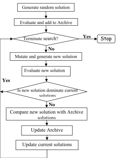
2.7.7.5 Pareto Archived Evolutionary Strategy (PAES)

This was first introduced by Knowles and Corne (2000a). The basic idea in this is shown by a flow chart (see Figure .2.15).

Initialize population and Pareto-optimal set, set gen=0 Start

Current Population

Determination of Nondominated solution

Extend Pareto set

Extend Population _{Reduce Pareto set by clustering}

Selection Crossover and Mutation

Size<Max. Size

Is feasible population

filled ?

Is gen <max gen

Update Pareto Set gen=gen+1 Yes No No Yes Yes Stop No

Figure 2.15: Flow chart of Pareto Archived Evolution Strategy (Knowles and Corne,

2000a)

This consists of a (1+1) evolution strategy (i.e., a single parent that generates a single offspring) in combination with Archive that records some of the non-dominated solutions previously found.

A new crowding method is introduced in this algorithm to promote the diversity in the population. The objective space is divided into hypercube by a grid in a recursive manner, which determines the density of individuals. Each solution is placed in certain grid location based on the values of its objective functions. A map of such grid is maintained, indicating the number of solutions that reside in each grid location. The zone with lower density is favored. Moreover the procedure has lower computation complexity

Generate random solution Evaluate and add to Archive

Terminate search? Stop

Mutate and generate new solution Evaluate new solution

Is new solution dominate current solutions

Compare new solution with Archive solutions

Update Archive

Update current solutions No

No

Yes