Mission Drift in Microcredit and
Microfinance Institution Incentives
Sara Biancini
David Ettinger
Baptiste Venet
CES
IFO
W
ORKING
P
APER
N
O
.
6332
CATEGORY 1: PUBLIC FINANCE
JANUARY 2017
An electronic version of the paper may be downloaded
• from the SSRN website: www.SSRN.com
• from the RePEc website: www.RePEc.org
CESifo Working Paper No. 6332
Mission Drift in Microcredit and
Microfinance Institution Incentives
Abstract
We analyze the relationship between Microfinance Institutions (MFIs) and external donors, with
the aim of contributing to the debate on “mission drift” in microfinance. We assume that both
the donor and the MFI are pro-poor, possibly at different extents. Borrowers can be (very) poor
or wealthier (but still unbanked). Incentives have to be provided to the MFI to exert costly effort
to identify the more valuable projects and to choose the right share of poorer borrowers (the
optimal level of poor outreach). We first concentrate on hidden action. We show that
asymmetric information can distort the share of very poor borrowers reached by loans, thus
increasing mission drift. We then concentrate on hidden types, assuming that MFIs are
characterized by unobservable heterogeneity on the cost of effort. In this case, asymmetric
information does not necessarily increase the mission drift. The incentive compatible contracts
push efficient MFIs to serve a higher share of poorer borrowers, while less efficient ones
decrease their poor outreach.
JEL-Codes: O120, O160, G210.
Keywords: microfinance, donors, poverty, screening.
Sara Biancini
Université de Caen Normandie
France - 14000 Caen
[email protected]
David Ettinger
Université Paris Dauphine
France - 75775 Paris Cedex 16
[email protected]
Baptiste Venet
Université Paris Dauphine
France - 75775 Paris Cedex 16
[email protected]
This version: January 2017.
We would like to thank Emmanuelle Auriol, François Bourguignon, Attila Tasnádi and seminar
participants at Oligo Workshop in Paris, the Canadian Economic Association Conference in
Ottawa and the European Development Network Conference in Bonn for helpful comments.
1
Introduction
For the last 30 years, the microfinance industry has been responsible for a massive growth of pro-poor financial services. The growth of the sector and the increasing financial flows into Microfinance Institutions (MFIs) have stimulate a debate on the evolution of the sector. The main elements of the recent evolution are the explosion of for-profit and profit-oriented MFIs and the change in the nature of some external donors (private vs. public). Both these issues have contributed to fuel the debate on the “mission drift” in microfinance. Armend´ariz et al. (2011) state that mission drift arises when a MFI “increases its average loan size by reaching out to wealthier clients neither for progressive lending nor for cross-subsidization reasons. Mission drift in microfinance arises when an MFI finds it profitable to reach out to unbanked wealthier individuals while at the same time crowding out poor clients”. Aubert, de Janvry, and Sadoulet (2009) define mission drift as a context where “MFIs increasingly tend to work with clients that are less poor”.
However, encouraging profitability is not necessarily a sign of abandoning the pro-poor orientation of microfinance. On the contrary, from the origin, financial sustainability and prof-itability have been considered as necessary conditions for a healthy development of microcredit markets. This clearly appears in Yunus (2007), when in its well known book “Banker to the Poor”, he states “If Grameen does not make a profit, if our employees are not motivated and do not work hard, we will be out of business. (...) In any case, it cannot be organized and run purely on the basis of greed. In Grameen we always try to make a profit so we can cover all our costs, protect ourselves from future shocks, and continue to expand. Our concerns are fo-cused on the welfare of our shareholders, not on the immediate cash return on their investment dollar.” (chapter 11, p. 204). Similarly, in the Key Principles in microfinance published by the Consultative Group to Assist the Poor (CGAP) in 2004, financial sustainability is evoked as the 4th principle and defined as “necessary to reach significant numbers of poor people”. In this spirit, observers and policymakers have increasingly put the accent on the necessity for microfinance institutions to be profitable, or “financially” sustainable, raising interest rates and going through commercialisation to be able to attract private investors (see Cull et al., 2009).
Nonetheless, a report commissioned by Deutschebank research showed that, in 2007, 70% of MFIs were small start-ups, mostly unprofitable, while only the top 150 MFIs were fully sustainable mature entreprises (Dieckmann et al., 2007). At the same time, the positive view of commercialization and profitability has been challenged in recent years by the critics following
the news that the largest microfinance bank in Latin America, the Mexican Compartamos, was offering returns on equity of 53%, while charging interest rates exceeding 100% to the poor. In a famous column appeared in the New York Times on January 14, 2011, Yunus reacted to this debate denouncing a tendency to “sacrificing microcredit for megaprofits”.
The main difficulty when trying to assess the extent of “mission drift” is that it is complicated to empirically establish whether a microfinance institution has indeed deviated from its poverty-reduction mission. One widely used proxy for poverty is average loan size, but as Armend´ariz et al. (2011) point out, the relationship between mission drift and loan size is not easy to tackle, so that socially responsible investors should be cautious when interpreting empirical evidence on loan size. Another possible sign of mission drift could be a tendency to practice higher interest rates. However, Roberts (2013) shows that, although profit oriented MFIs do usually charge higher interest rate, they are not significantly more profitable, because they tend to have higher costs. He concludes that his analysis finds “no obvious indication of a mission drift”.
We believe that additional theoretical work is needed to understand the phenomenon and being able to interpret empirical facts. In the present paper, we present a theoretical analysis aimed at increasing our understanding of the role of donors in affecting mission drift tendencies in microfinance. We propose a model in which both the donor and the MFI are pro-poor, although they can put different weights on the aim of providing credit to the poorest borrowers. Incentives have to be provided to the MFI to exert costly effort to identify the more valuable projects and to choose the right share of poorer borrowers (the optimal level of poor outreach). We characterize the optimal contract proposed to MFIs in the aim of balancing outreach, budget considerations and MFIs survival.
We consider both the cases of hidden action (effort is not observable) and hidden types (MFIs have unobservable cost heterogeneity). The two cases are relevant for the sector. For instance, the report “Microfinance in Africa” realised for the United Nations in OSAA and NEPAD (2013), put the accent on the difficulties of operating in a context of lack of transparency and weak institution, an environment which favor hidden action problems. In addition, the same report also points out that the donors should promote the diversification of institutions to “improve range and quality of services, and reduce costs”. This suggest the importance of the role of donors in proposing differentiated contracts in a context of heterogeneous institutions as in our framework with hidden types. Hidden type problems are also likely to be very relevant in context like Latin America, where microcredit providers present a wide range of institutional diversity and performances (see for instance the recent Report of Trujillo and Navajas, 2014).
We first assume that effort is unobservable (hidden action model) assuming that the donor cannot observe neither the effort level chosen by the MFI, nor the fraction of richer borrowers. He only discovers the total repayment rate of loans to the MFI. We show that, in this case, asymmetric information can reduce the share of very poor borrowers reached by loans, thus increasing mission drift. This happens when the pro-poor orientation of the MFI is weak as compared to the one of the donor, so that this source of mission drift is more likely to arise in country in which MFIs are profit oriented. Afterwards, we allow for unobserved heterogeneity among MFIs: some of them are more efficient than others and the contract proposed by the donor has to screen among different types of MFI (hidden type model). In this case, the existence of asymmetric information between the donor and the heterogeneous MFIs tends to increase the poor outreach of the more efficient MFIs while decreasing it for less efficient ones so that in some case asymmetric information has the effect of lowering the average level of mission drift (i.e. the share of richer borrowers who are granted a loan).
1.1 Related literature
The question of the relationship between MFIs and external donors has gained importance in the last year. Surprisingly, as Ghosh and Van Tassel (2013) point out, the existing literature on microfinance has not paid much attention to that question1. An indirectly related literature has considered the broader question of the relationship between external donors and other recipients (such as NGOs). For instance, Besley and Ghatak (2001) consider the issue of the optimal contract between a government and an NGO to carry out a development project, showing how hold-up problems shape the optimal way to delegate responsibility for providing social welfare and development services to nongovernmental organizations. Aldashev and Verdier (2009, 2010), examine the effects of international competition between NGOs to raise funds. They show that if the level of outside options of NGO entrepreneurs is low enough, increased competition among NGOs can lead to higher fund diversion, despite the fact that they care about the impact of their projects.
More recently, the literature has tackled specific issues of microfinance. In this context, Aubert, de Janvry, and Sadoulet (2009) focus on the internal organization of MFIs and highlight the importance of the incentives given to the credit agents. They analyze the optimal contract in the presence of moral hazard and investigate the issue of mission drift in this context. In their model, the credit agents are not pro-poor and can under-report repayments so that they
1Most papers are dedicated to the contracting between MFIs and their clients: see Ghatak and Guinnane
have to be given the right incentives to investigate the ability and wealth of borrowers. The MFI can monitor agents. However, when monitoring is costly, a pro-poor MFI can be obliged to provide the agent with incentives based on repayments thus generating mission drift. While Aubert, de Janvry, and Sadoulet (2009) concentrate on the internal incentives provided by MFIs, incentive issues are also likely arise in the relationship between MFIs and external donors. In our paper, we concentrate on this relationship as a source of contract frictions and mission drift. In our context, we find reasonable to assume that both the MFI and the donors are pro-poor, at least to some extent. Although we do not allow the MFI to under-report repayments, in our framework, incentives need to be provided to have the MFI exerting costly effort to discover valuable clients’ investment projects (while wealth is easily observable by the MFIs which has better knowledge than the donors of the local conditions). In this context, in addition to moral hazard problems we also consider adverse selection issues. MFIs are heterogeneous and the donor cannot perfectly observe their characteristics. In our context, asymmetric information and contract distortions can have different impacts on mission drift.
Ghosh and Van Tassel (2011, 2013) also focus on the relationship between donors and MFIs. In their first paper, they present a model in which socially responsible MFIs (their main goal is to reduce poverty) must be funded by a profit-seeking investor. They find that competition among MFIs to obtain external funds has two opposite effects: on the one hand, having to pay a high rate of return to the external funder raises the interest rates charged to borrowers; on the other hand, it is also a way to make the funding more efficient by redirecting funding from inefficient MFIs to more efficient ones. If the average increase in the quality of MFIs more than compensates for the higher interest rates, the competition for external funds is pro-poor. In our paper, we do not consider competition and we assume that the donor also has a social objective. We show that the optimal contract proposed to heterogeneous MFIs does not necessarily exclude inefficient MFIs, unless there are very few of them. We characterize separating contract in which efficient and inefficient MFIs are optimally proposed different contracts. Moreover, we consider asymmetric information.
Our approach is thus similar to Ghosh and Van Tassel (2013), who extend the previous analysis by introducing asymmetric information and socially motivated donors. In their analysis, the financial return may be used as a screening mechanism by donors to discriminate between MFIs, dissuading high cost MFIs to apply for external funding. In our framework, we show that exclusion of the less efficient MFIs occurs only if their number is small. Otherwise, the donor may propose different contracts to different types of MFIs, which may have different
impacts on mission drift. Incentives will be provided not to squeeze out the less efficient MFIs, but to promote effort and to screen among heterogeneous MFIs proposing different contracts to different types of MFIs. In addition, we assume that the donor cares for the survival and long term viability of MFIs, putting a positive weight on the profit of the MFI. This captures the idea that leaving some money to a MFI is not completely wasteful for the donor, because it allows the MFI to survive in the future.
2
The basic model
We consider the relationship between a donor (the principal, “he”) and an MFI (the agent, “she”). The MFI lends a mass 1 of money to a local population of borrowers. The population of borrowers contains an infinity of borrowers, who don’t have access to bank lending. Borrowers are heterogeneous: some of them are richer (they are unbanked but less poor, with a positive initial wealth level that is not pledgeable and does not allow to access bank lending) and some of them are poorer (they have no wealth whatsoever). The MFI chooses the proportion α of the money lent to richer borrowers in his loans portfolio and the weight she puts on financing the right level of poorest borrowers measures her pro-poor orientation. In addition, the MFI has to exert effort to screen out valuable projects, when examining the project proposed by both richer and poorer borrowers. This effort level e can be interpreted as the share of loans for which the MFI makes costly effort in order to identify the quality of the project. Without any screening effort on the MFI side, the expected reimbursement of richer borrowers, RR,
is strictly higher than the expected reimbursement of poorer borrowers, RP, because richer
borrowers have higher collateral. We also assume that the screening effort increases the loans return by a parameter, ∆R and for simplicity we assume that this parameter is identical for richer and poorer borrowers.
The expected reimbursement for the projects financed by the MFI is therefore equal to:
θ(α, e) = RP + α(RR− RP) + ∆Re (1)
With e, the fraction of loans for which the MFI exerts a screening effort. We assume that the cost associated to the effort e is linear and does not depend on the type of borrowers so that we can denote it µe with µ > 0. This effort translates into a monetary cost, because in order to identify the quality of the borrower projects, the MFI has to pay credit officers who study the quality of the projects. The effort provided by the MFI can thus be simply interpreted
as an effort necessary to examine projects and screen the good ones (with higher repayment potentials). Alternatively, this can be interpreted as the effort (and the cost) necessary to provide additional services to the borrowers, thus increasing the potential of their investment projects.
In order to finance the loans, the MFI has no direct access to the financial market so that she has to contract with a donor (the principal). The donor proposes a contract or a menu of contracts to the MFI. The contract specifies the refund, T , that the MFI is supposed to pay to the donor in exchange for the funding and, depending on the informational context that we will specify the effort level, e.
The donor’s utility is an increasing function of the refund he receives from the MFI but the donor is also concerned by the loan allocation to the right borrowers and the survival of the MFI. More precisely, we represent his preferences with the following utility function:
V = T − 1 + λ1 ( 1− (α− α ∗ 1− α∗) 2)+ λ 2(θ(α, e)− µe − T ) (2)
T − 1 is the budget balance of the lending process for the donor. λ1 > 0 is the weight that
the donor puts on the distribution of the loans to the right borrowers. α∗is the optimal fraction of loans granted to richer borrowers. α∗ is not necessarily equal to 0. For several reasons, the donor may prefer that some richer borrowers may also be financed.2
We choose the formula (1− (α1−α−α∗∗)2) to represent the utility that the donor derives from
lending money to borrowers with a fraction of richer borrowers because we wanted to make it clear that the donor derives a positive utility from lending this money. In the version we use, this element that we incorporate in the utility function is always positive. However, after some normalization, we can show that this is equivalent to considering −(α − α∗)2 which is simpler.
(θ(α, e)−µe−T ) is the amount of money left to the MFI and λ2 ≥ 0 is a parameter representing
the interest of the donor in the survival of the MFI. The higher θ(α, e)− µe − T , the higher the net income of the MFI and her probability to survive. We assume that λ2 < 1, otherwise the
donor could increase his utility by simply transferring money to the MFI.
2
Different values for the optimal share of poorer borrowers can derive from natural welfare functions in which the donor cares for the welfare of the poorest borrowers, while taking into account that richer unbanked borrowers generates higher expected income. For instance, even if the donor only cares about poorer households, she might take into account that lending to some richer individual might generate a trickle-down effect, for instance creating local jobs and increasing the living condition of the poorer borrowers. On the other hand, even if richer households produce higher expected revenue, the donor would want to finance a certain ratio of poorer borrowers to achieve a better distribution of wealth. In addition, unbanked wealthier are relatively more abundant than unbanked poor in many middle-income regions. As noted in Armend´ariz et al. (2011) the fact that many MFIs in these region serves a higher share of less poor borrowers does not necessarily means that they all deviated from their mission.
The MFI also cares about the ratio of poorer and richer borrowers to whom she grants loans. For the sake of simplicity, we assume that the preferred fraction of richer borrowers for the MFI is the same as for the donor, α∗.3 However, the weight that the MFI gives to this dimension of his utility β1 > 0, may differ from the λ1 of the donor. Eventually, the MFI’s utility function is
defined as follows. U = θ(α, e)− T − µe + β1 ( 1− (α− α ∗ 1− α∗) 2) (3)
Besides, we assume that the MFI has no other external funds at the time she accepts the contract with the donor so that she also faces a budget constraint:
θ(α, e)− T − µe ≥ 0 (4)
The MFI does not accept a contract such that this constraint is not satisfied (perfectly anticipating her own behavior after having accepted the contract).
3
First case: the donor cannot observe effort e (Hidden action)
In this section, we assume that the donor cannot observe neither the effort level chosen by the MFI, e nor the fraction of richer borrowers, α. However, the donor discovers the reimbursement level, θ, obtained by the MFI (the MFI cannot hide the money). We also assume that e can take any value in the interval [0, 1] and that the value of µ is common knowledge. The timing of the game is the following:
• Step 0: The donor makes an offer (θc, Tc) to the MFI. The offer may be interpreted as:
I propose you a capital of 1 in order to lend money to local borrowers. If I observe that you obtain a reimbursement rate equal to θc, I ask you a repayment Tc. If I observe a reimbursement rate different from θc, I ask you a repayment T > θ(1, 1) and you go
bankrupt.
• Step 1: The MFI accepts the offer or refuses it. If she refuses it, the game is over without any lending or transfers. If she accepts it, the game continues.
• Step 2: The MFI chooses e and α. 3
We could also obtain results with an α∗M F I and an α∗D and α∗M F I ̸= α∗D. However, we chose to consider a
unique α∗in order to show that our results cannot be explained by the different view about the optimal fraction of richer borrowers between the MFI and the donor. Hence, the choice of a unique α∗.
• Step 3: Borrowers reimburse the loan. θ(e, α) is common knowledge and the MFI makes her payment to the donor in accordance with the initial contract and the actual value of θ.
This game is aimed at representing, in a simple framework, a situation in which the donor cannot observe the actual effort made by the MFI to discover good projects (or to propose valuable services to borrower) nor the actual wealth of the borrowers. On the other hand, we can think that the donor can more easily observe the total revenue of the MFI and propose a reimbursement of the funds which is a function of the realized revenues, that, for simplicity, we assume to be perfectly observable.
Before focusing on the contract and the decisions of the MFI, we first observe that it is not necessary to consider values of θc such that θc< RP + α∗(RR− RP) since both the donor and
the MFI agree that α < α∗ gives a lower utility and a lower reimbursement level than choosing α = α∗.
Now, let us consider the MFI decision. Since the contract only specifies θc, the reimburse-ment level, if she accepts it, she will choose among all the pairs (e, α) such that θ(e, α) = θc. In order to increase the size of the reimbursement rate, increasing the share of rich borrowers is a substitute to higher effort.
If θc≥ RP+ α∗(RR− RP), the MFI will choose an α such that α≥ α∗ so that the marginal
cost of increasing θ by rising the fraction of richer borrowers is 2β1 RR−RP
α−α∗
(1−α∗)2 which is strictly
increasing in α. The MFI increases α up to the point when further increasing the share of richer borrowers becomes more costly than increasing effort. The marginal cost of increasing θ by a raise in the effort level is equal to ∆Rµ which is a constant. The two costs are equal when α = α∗+(1−α∗)2(RR−RP)µ
2β1∆R ≡ α
M. Therefore, there are 3 cases (assuming that Tcis small
enough, otherwise the MFI will refuse the contract): • If θc< R
P+ αM(RR−RP), the MFI will choose an effort level 0 and an α equal to θ
c−R
P
RR−RP
in order to obtain θc.
• If RP + αM(RR− RP) ≤ θc≤ RP + αM(RR− RP) + ∆R, the MFI will choose α = αM
and an effort level e∈ [0, 1] such that the reimbursement level is equal to θc. • If θc> R
P + αM(RR− RP) + ∆R, the MFI will choose an effort level 1 and an α equal
to θc−RP−∆R
RR−RP in order to obtain θ
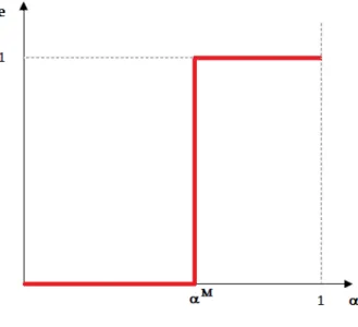
This result appears on Figure 3 which represents all the pairs (α, e) chosen by the MFI depending on the θc proposed by the donor. When the graph goes northeast, this coincides with a higher θc chosen by the donor. The graph is uniquely characterized by the value of αM.
Figure 1: MFI’s preferences
Now, the donor. We first consider the donor’s first best, the choice that he would impose on the MFI if he could choose the pair (α, e) which maximizes his utility while satisfying the MFI budget constraint, T ≤ θ(α, e) − µe. This constraint will always be binding since λ2 < 1,
therefore we can assume that in this first best contract, T = θ(α, e)− µe so that the donor’s utility will be equal to:
V = RP + α(RR− RP)− 1 + ∆Re − µe + λ1 ( 1− (α− α ∗ 1− α∗) 2) (5)
This is equal to the utility of the MFI given in (3), except that T (the transfer for the MFI) is replaced by 1 and the parameter β1 is replaced by λ1.
Looking at the formula, we observe that if ∆R < µ, the donor prefers e = 0, if ∆R > µ, the donor prefers e = 1 and if µ = ∆R, the donor is indifferent among effort levels. As for the optimal level of α, we can find it by maximizing α(RR− RP) + λ1(1− (α−α
∗
1−α∗)
2). This gives an
optimal α for the donor: α∗+(1−α∗)2(RR−RP)
2λ1 ≡ α D.
Now, the donor cannot actually choose the pair (α, e) because he does not observe the choice of the MFI. We can consider 3 different cases.
If ∆R ≤ µ, the cost of effort is higher than the social benefit, the donor prefers (αD, 0). Preferring that the MFI makes no effort, the donor can propose a contract which only
cov-ers the costs with no effort when the share of richer borrowcov-ers is equal to αD, (θc, Tc) = (θ(αD, 0), θ(αD, 0)). The MFI will accept the contract and choose (α, e) = (αD, 0) so that the donor will manage to impose his preferred pair to the MFI.
If ∆R > µ and αD ≥ αM, the cost of effort is lower than the social benefit and the optimal α for the donor is higher than the optimal α for the MFI. The donor can obtain that the MFI chooses (α, e) = (αD, 1) by proposing a contract (θc, Tc) = (θ(αD, 1), θ(αD, 1)−µ). In this case, the donor can obtain the preferred share of richer borrowers by imposing a high reimbursement which forces the MFI to exert effort and to push the share of richer borrowers to αD.
Now the richest case is when ∆R > µ and αD < αM. Since ∆R > µ, the donor would prefer the MFI to make an effort equal to 1 (the social cost of the effort is lower than the social profit). The donor would also like the MFI to choose an α strictly lower than αM since αD < αM. However, we already noted that whatever the contract proposed (θc, Tc), it is never possible to
obtain that the MFI chooses an effort equal to 1 and an α < αM since the MFI will always reduce its effort (with a marginal cost ∆Rµ for an increase in θ) and raise the ratio, α of richer borrower (with a marginal disutility for an increase in θ strictly lower than ∆Rµ when α < αM). Therefore, we obtain the following result.
Proposition 1 The donor proposes a contract (θc, Tc) to the MFI such that:
• If ∆R ≤ µ, the donor proposes a contract inducing effort e = 0, setting θc= θ(αD, 0) and Tc= θ(αD, 0).
• If ∆R > µ and λ1 > ∆Rµ β1 (equivalent to αD ≥ αM), the donor proposes a contract
inducing effort e = 1, setting θc= θ(αD, 1) and Tc= θ(αD, 1)− µ. • If µ ≤ ∆R < µ + λ1(αM−αD)(αM+αD−2α∗)
1−α∗ + (αM − αD)(RR− RP) and λ1 ≤ ∆R
µ β1, the donor proposes a contract inducing effort e = 0, setting θc= θ(αD, 0) and Tc= θ(αD, 0). • If ∆R > µ +λ1(αM−αD)(αM+αD−2α∗)
1−α∗ + (α
M− αD)(R
R− RP) and λ1 ≤ ∆Rµ β1, the donor
proposes a contract inducing effort e = 1, setting θc= θ(αM, 1) and Tc= θ(αM, 1). In all cases the MFI accepts and executes the proposed contract.
If the social cost of effort is high, µ ≥ ∆R, there is no effort and no distortion due to the asymmetry of information. The donor can implement the lending policy he prefers even if he only observes θ. Even if αM < αD so that in order to obtain the reimbursement rate θ(αD, 0) which would coincide with the preferred choice of the donor (αD, 0), the MFI would rather make
strictly positive effort and choose an α strictly lower than αD (as can been seen with point A and A’ in Figure 2(a)), the donor can implement (αD, 0). The MFI will never make any effort if she is not compensated for this effort because of her budget constraint. If the donor wants to implement point A, although the MFI would prefer point A’ (with the same θ), the donor can force the MFI to choose A.
The α chosen is not equal to α∗ which may be considered as a mission drift. This is explained by the tradeoff between lending money to poorer borrowers and obtaining a higher reimbursement rate. Since the cost of an increase in the fraction of richer borrowers at the neighborhood of α∗ is negligible and the marginal increase in reimbursement rate is constant, equal to RR− RP, the chosen α will always be higher than α∗.
If the social cost of effort is lower than its social benefit, µ < ∆R, it is socially optimal to make an effort equal to 1. However, this effort will not always be implemented. If αD is higher
than αM, the situation is simple, the donor proposes a contract with an α = αD, e = 1 and a repayment such that the MFI makes no profit. Since (αD, 1) is an element of the optimal curve
of the MFI, he will accept the contract and choose (αD, 1). This is represented by point B in Figure 2(a).
Now, if αD < αM and the donor proposes a contract (θ(αD, 1), θ(αD, 1)− µ), the MFI will not choose (αD, 1). He will choose a lower effort level and a higher α.
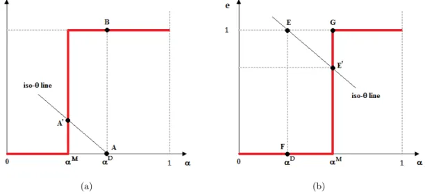
(a) (b)
Figure 2: MFI’s preferences and optimal contracts under hidden action.
As we can see on Figure 2(b), if the donor proposes a contract (θ(αD, 1), θ(αD, 1)− µ) with α < αM (such as the one denoted by point E in the Figure 2(b)), the MFI will substitute effort for a higher proportion of richer borrowers (choosing E′). Therefore, the donor cannot do better
than choosing between 2 solutions. He can either obtain that the MFI chooses αD by proposing a contract (θ(αD, 0), θ(αD, 0)) (corresponding to point F in Figure 2(b)) but no effort will be made or he can propose (θ(αM, 1), θ(αM, 1)− µ) (corresponding to point G in Figure 2(b)) so that the effort level will be equal to 1 but the fraction of richer borrowers will be higher than the donor’s first best. In the first case, the effort level is suboptimal, in the second case, the fraction of richer borrowers is too high, a stronger mission drift. The donor will choose among these two contracts the one that minimizes his utility loss.
The model thus shows how mission drift is affected by the objectives of the donor and the MFI. As expected, a high share of richer borrower can depend on the preferences of the donor. If the donor puts a low weight on the pro-poor mission, then he can decide to push the MFIs to realize his preferred share of poor borrowers asking for a high reimbursement, so that effort alone is not enough for the MFI to generate the required revenue and she is pushed to serve more richer borrowers. The hidden action problems can have an additional (adverse) impact on the mission drift as compared to the benchmark case of complete information. This happens when the MFI put relative low weight on the pro-poor mission while the donor is more pro-poor (as in the case illustrated in Figure 2(b)): in this case, the donor cannot induce the preferred share of poorer borrowers and mission drift increases (as in point G). Alternatively, the donor has to renounce to induce high effort (as in point F ). This could also be interpreted as an other source of mission drift in the sense that, for a given share of richer borrower, the quality of the service provided by the MFI has to be degraded to satisfy the contract proposed by the donor. We have thus shown that hidden action is likely to have an adverse effect on mission drift when the pro-poor orientation of the MFI is weak compared to the one of the donors. On the contrary, if the MFI is pro-poor, the contract proposed by the donor can induce the desired level of effort and of the share of reacher borrower desired by the donor so that asymmetric information has no particular impact on the mission drift.
To drive some implications from the model, it is first important to note that hidden action is related to the unobservability of effort. In practice, this problem is more relevant when the market is less transparent and the information on the functioning of MFIs is hard to gather. For instance the report “Microfinance in Africa” (OSAA and NEPAD, 2013) mentions that a widespread weakness of African Microfinance is the prevalence of governance problems coupled with the diffusion of informal enterprises with scarce access to reliable information. In these countries, governments and development institutions should thus probably concentrate their efforts in increasing transparency and support MFIs to improve governance. In addition, we
have shown that the distortions are driven from the weak pro-poor orientation of MFIs. In a context in which many MFIs are profit-oriented, like in many Latin American countries for instance, the presence of hidden action is more likely to worsen the mission drift. But things should be different in Asian countries like India and Pakistan with a traditional focus on the social mission (Report on Asian Microfinance edited by Bedson, 2009). This is not to say that moral hazard cannot occur in pro-poor MFIs, but in our framework we show that in this case it is easier for the donors to obtain the desired levels of effort and redistribution through second best contracting with the MFIs.
4
Second case : the donor cannot observe the type of the MFI
θ (Hidden type)
In this section, we consider the case in which MFIs are characterized by unobservable hetero-geneity. For simplicity, we assume that there are two types of MFIs, a share η of more efficient ones with low cost of effort µL, and a share (1− η) of less efficient MFIs with high cost of effort µH > µL. To simplify the analysis, we assume in this section that effort is observable and can take two values, ei ∈ {0, 1}, i = 1, 2. We thus restrict our attention to the hidden type problem
faced by the donor. The donor cannot observe the cost of effort of the MFI but he can offer a menu of contracts possibly discriminating between the different types of MFIs. We assume that the donor offers a contract depending on the type of MFI (H, L) in such a way that each MFIs prefers the contract designed for her type rather than the contract designed for the other type (the Revelation Principle ensures that restricting the attention to this kind of contracts is without loss of generality). Thus, in step 0, the donor proposes a menu of contracts depending on the MFI’s type (θH, TH, eH), (θL, TL, eL). The other steps are unaffected.
Because types are unobservable, the proposed contracts have to satisfy an incentive compati-bility constraint, to avoid that MFIs mimic a cost of effort different from the true one. As well known, incentives for truthful revelation generally generate additional costs for the principal (the donor) in terms of rents abandoned to the agents (the MFI) and in terms of contract dis-tortions. In some cases the principal (the donor) might also decide to offer the same contract to both types (pooling equilibrium) instead of tailoring the contract on the different cost char-acteristics, when the distortions created by the separating contracts are too large.
V = η [ TL− 1 + λ1 ( 1− (α L− α∗ 1− α∗ ) 2)+ λ 2(θ(αL, eL)− µLeL− TL) ] +(1− η) [ TH− 1 + λ1 ( 1− (α H − α∗ 1− α∗ ) 2)+ λ 2(θ(αH, eH)− µHeH − TH) ] (6) Under the two budget constraints:
θ(αL, eL)− TL− µLeL≥ 0 (7)
θ(αH, eH)− TH − µHeH ≥ 0 (8)
And the incentive compatibility constraints:
θ(αL, eL)− TL− µLeL+ β1(1− ( αL− α∗ 1− α∗ ) 2)≥ θ(αH, eH)− TH − µLeH + β 1(1− ( αH − α∗ 1− α∗ ) 2) (9) θ(αH, eH)− TH − µHeH + β1(1− ( αH− α∗ 1− α∗ ) 2)≥ θ(αL, eL)− TL− µHeL+ β 1(1− ( αL− α∗ 1− α∗ ) 2)(10)
For standard reasons, at the optimal solution, the budget constraint of type H (8) and the incentive compatibility constraint of type L (9) will be binding so that we can replace in the objective function of the donor (6) the values of the transfers:
TH = θ(αH, eH)− µHeH (11) TL = TH + β1 [ (α H− α∗ 1− α∗ ) 2− (αL− α∗ 1− α∗ ) 2]+ (θ(αL, eL)− θ(αH, eL)) + eH(µH − µL)(12)
Replacing (11), (12) and (1) in (6) we obtain:
V = η [ λ1(1− ( αL− α∗ 1− α∗ ) 2) + ∆R + R P + αL(RR− RP)− µLeL− 1 ] +(1− η) [ λ1(1− ( αH− α∗ 1− α∗ ) 2) + ∆R + R P + αH(RR− RP)− µHeH − 1 ] −η(1 − λ2) [ β1[( αH − α∗ 1− α∗ ) 2− (αL− α∗ 1− α∗ ) 2] + eH(µH − µL)] (13)
Because the MFI revenue θ(αi, ei) and her effort ei, i = {1, 2} are observable, maximizing (6) with respect to Ti, θ(αi, ei) and ei corresponds to maximizing with respect to ei and αi equation (13) subject to the residual constraints (7) and (10).
The last term in the donor’s objective (13), β1[(α
H−α∗
1−α∗ )2−(
αL−α∗
1−α∗ )2]+eH(µH−µL), represents
the information rent of the most efficient type L. Efficient MFIs get a (weakly) positive rent from their information advantage. This rent is null if and only if µHeH = µLeL (which can
occur only if eH = eL = 0) and αH = αL. The objective function of the donor is decreasing in the information rent, but its weight in donor’s utility is decreasing in λ2 (the higher λ2 the
more the donor is willing to abandon positive profits to the MFIs to ensure their survival and thus the less costly is the information rent in terms of utility for the donor). The donor can choose to induce equal or different effort level and propose different or equal transfers (and thus shares αi, i∈ {H, L}).
Proposition 2 Depending on the value of the parameters, the optimal menu of incentive-feasible contracts takes one of the following forms:
Type 1: The donor induces no effort for both types (eH = eL = 0). The share of richer
borrowers are αL = αH = αD. Transfers are equal for the two types of MFI, TH = TL = θ(αD, 0).
Type 2: The donor induces effort only from the efficient type L (eH = 0, eL = 1). The
shares of richer borrowers are αL = αH = αD respectively. The transfer from the less efficient MFI is TH = θ(αD, 0) and TL = θ(αD, 1)− µL (or more precisely TL is arbitrarily closed to θ(αD, 0)− µL).
Type 3: The donor induces effort from the two types (eH = eL= 1) and proposes a separating
contracts with different shares of richer borrowers αL< αH and TL< TH.
Proof : see Appendix Analysis.
Type 1 contract (no effort) is optimal if and only if ∆R < µL. Otherwise, the principal would induce effort of at least the more efficient type L.
If µL≤ ∆R ≤ µH the donor proposes a type 2 contract, inducing high effort only for type L, because effort of type H is too costly to be desirable. This type of contract does not generate any information rent and allows the donor to obtain its preferred share of richer borrowers αD. Because type H is not incited to exert effort, its contract is not attractive for type L, who will be indifferent between the contract for type H MFI and the one proposed for its type. Similarly, type H is not attracted by the contract proposed to L because this contract does not allow to cover a high cost of effort µH.
The richest case is the one in which ∆R > µH. In this case, effort of the two types of MFI is socially efficient, it would always be induced under complete information. However, under asymmetric information the principal needs to satisfy the incentive compatibility constraint (9), which becomes costly because an MFI of type L has a lower cost of effort and an incentive to pretend to be of type H.
Therefore, in order to obtain that both types of MFI make the effort, it is necessary to leave an information rent to the efficient MFIs. Even when ∆R > µH, it may be the case that the donor prefers a type 2 contract in which inefficient MFIs do not make the effort in order to reduce the information rent given to efficient MFIs. This will be the case if ∆R− µH (the efficiency gain associated to the effort of an inefficient MFI) and 1− η (the proportion of inefficient MFIs) are low.
However, for reasonable values of the parameters of the model, the optimal contract for the donor will be a separating type 3 contract in which both types of MFI make the effort. This requires that ∆R > µH which means that effort of the less efficient type also bring some
efficiency gain, and that 1− η is not too small, which means that there is not a overwhelming majority of more efficient MFIs. We will elaborate on type 3 contracts in the remaining part of this section.
Let us first consider the nature of these contracts. The donor wants both types of MFI to make the effort. In order to do so, he may propose the following two contracts: (eH, αH, TH) = (1, αD, θ(α, 1)− µH) and (eL, αL, TL) = (1, αD, θ(α, 1)− µL). But both types of MFI would choose the first contract pretending to be inefficient and obtaining to pay back to the donor the lower amount of money θ(αD, 1)− µH. In order to deter efficient MFIs from choosing the contract designed for inefficient ones, the donor has to make the contract designed for inefficient MFIs less attractive. A natural way to do so, since TH cannot be lower than θ(αD, 1)− µH (otherwise inefficient MFIs will not be able to cover their costs) is to increase αH. Lowering the fraction of loans provided to poorer borrowers is costly for the MFI who also cares about the ratio of poorer and richer borrowers financed by his loans. Then, an efficient MFI will prefer a contract with α = αD and a higher T rather than the contract designed for inefficient MFIs with both a higher T and a higher α. As a result, we observe a stronger mission drift with an α > αD when the MFI is inefficient even though both the MFI and the donor would prefer α to be equal to αD. This mission drift is explained by the hidden type of the MFI. The donor chooses the stronger mission drift as a way to reduce the information rent given to the efficient type.
Now, this is not the end of the story. Usually, in the principal-agent theory, the no distortion at the top rule applies. The contract designed for the most efficient agent is not distorted, not affected by the asymmetric information (except for the amount of the transfer). A natural interpretation of this rule in the environment we consider would be that the contract proposed to the efficient agent should specify an effort level and an α equivalent to the one we would observe with perfect information: e = 1 and α = αD. This is not the case. It is possible here to obtain a contract which is socially preferable to the one obtained in the perfect information case.
For the sake of simplicity, we will first present the intuition for the case λ2 = 0. Suppose
that the donor wants both types of MFI to make the effort and α to be equal to αD. He
can obtain this outcome with a contract (e, α, T ) = (1, αD, θ(α, 1)− µH). Both types of MFI accept the contract and efficient MFIs obtain a revenue equal to µH − µL. This means that
efficient MFIs are no longer budget constrained. Then, the donor could propose a contract (1, αD − ε, θ(αD − ε, 1) − µH + ε(2αD−2α∗−ε)β1
(1−α∗)2 ),
ε(2αD−2α∗−ε)β1
(1−α∗)2 , being the MFI’s increase in
utility when α decreases from αD to αD− ε. This contract can be interpreted as follows. The donor proposes to efficient MFIs a reduction of α and an increase in the money that he is paid back by an amount equivalent to the increase in utility obtained by reducing α. This means that the donor derives both his extra utility by lowering α and the extra utility that the MFI derives by lowering α (through the increase of T ), a total equal to (λ1+β1)(α
D−α∗)2−(αD−ε−α∗)2
(1−α∗)2 .
If the donor receives all the social surplus associated to a decrease in α, his optimal value of α is no longer αD but it coincides with the social optimal value of α (taking into account the MFI and the donor’s preferences): αD+M F I ≡ α∗+ (1−α∗)2(RR−RP)
2(λ1+β1) < α
D so that the donor is
better off if the efficient MFI accepts the contract (as long as αD− ε ≥ αD+M F I) and the MFI will accept it as long as ε(2αD−2α∗−ε)β1
(1−α∗)2 ≤ µH− µL(otherwise the budget constraint is no longer
satisfied and she goes bankrupt).
This explains why in the optimal contract designed for the efficient MFI, the α is strictly lower than αD, getting closer to αD+M F I, the value of α which maximizes the joint utility of the donor and the MFI. Distorting downwards the share of richer borrowers served by the efficient MFI, the donor can obtain an higher surplus, so that he always chooses to do it in the optimal contract.
Because at the optimal contract the share of richer borrowers is distorted upwards for the inefficient MFIs an lower for the inefficient, the total share of richer borrower can be lower or higher than the one prevailing under complete information. The impact of hidden types on
mission drift is thus ambiguous. Intuitively, if the share of efficient MFIs, η, is high enough, then the average share of richer borrowers served by the two types of MFI would decrease, because the downward distortion of α would prevail for a large number of contracts. To see this, we have computed the share of richer borrower α = ηαL+(1−η)αH and compared it with the benchmark level αD (obtained under complete information) in anumerical example. As an illustration, if we set α∗ = 0.2, β1 = λ1 = 0.3, λ2 = 0, RP = 0.5, RR = 0.1, ∆R = 0.7, µH = 0.4, µL = 0.1,
then the average share of richer borrowers α is lower than αP whenever the share of efficient MFI η is higher than 0.5. Thus, in this example if more than one half of the MFI are efficient, mission drift is reduced when information is asymmetric. The same qualitative behavior holds in general (but of course the particolar threshold of η moves when modifying the values of the parameters), as shown in the Appendix.
In our context, in which both the MFI and the donor are pro-poor (although they can put different weight on pro-poor orientation and also care about revenues), incomplete information can deliver a result which is socially more desirable than complete information. The necessity to discriminate among MFIs types pushes the donor to decrease the share of richer borrower served by more efficient MFI while demanding higher transfers to compensate for this deviation from the preferred level αD. This allows the donor and the MFI to increase efficiency and may have an unexpected beneficial effect on the pro-poor orientation of lending activities (when the average share of poorer borrowers is increased).
Discussion.
A noticeable feature of the hidden type problem is that the impact of asymmetric information does not necessarily go in the direction of increasing the mission drift with respect to the benchmark case of complete information. As shown above, in the separating equilibrium with different shares of richer borrowers, this share is distorted upwards for the inefficient MFI but downwards for the more efficient.
At the separating contract of type 2 with equal shares of richer borrower, the shares are not distorted with respect to full information. However, the agency problem of the donor induces an inefficiently low level of effort for high cost MFIs. This can be perceived as a higher difficulty for some types of (relatively inefficient) MFIs to increases services to poor borrowers, when contracting with an external donor.
Hidden types issues are particularly relevant in markets in which the level of heterogeneity among MFI is high. This is for instance in many Latin American countries, as stressed for instance in the recent report by Trujillo and Navajas (2014). In this context, our analysis could
offer arguments to suggest that governments and development institutions have a role to play to help MFIs to build capacity, provide better services and increase efficiency. In our model, to discriminate among MFIs under hidden types, the donor must set the contract such as the share of richer borrowers is smaller for more efficient MFIs. This allows the donor and the MFI to increase efficiency and may have an unexpected beneficial effect on the pro-poor orientation of lending activities. This indirect positive effect can occur if number of efficient MFIs is large enough and it is greater when their number increases. Therefore, governments and development institutions aiming to strengthen the fight against poverty could play a role by helping MFIs to increase their efficiency.
It is also worth noting that the optimal menu of contracts of type 3 could also be interpreted as follows. For less efficient MFIs , the donor imposes a level αH and get all the revenue minus µH. In a sense, the donor covers exactly all the MFI’s costs assuming that she is inefficient. For
more efficient MFIs, the donor also imposes α but a lower level, αL and state a fix repayment rate so that the most efficient MFIs freely choose to exert the effort and keeps a positive margin.4
5
Conclusion
The present paper contributes to the debate on the recent evolution of the microfinance sector, fueled by the explosion of for-profit and profit-oriented MFIs and by a change in the nature of some external donors (private vs. public). The entry of new market players raises the fear for a deviation from the poverty-reduction mission, the so-called “mission drift”. We build a model in which we analyze the relationship between donors and MFIs, assuming that both are pro-poor. Assuming that the effort to screen valuable investment projects is costly, incentives have to be provided to the MFI by the donor to exert the right effort level and to choose the desired share of poorer borrowers. We first concentrate on hidden action issues. We show that, in this context, asymmetric information can reduce the share of poorer borrowers reached by loans, thus increasing the mission drift.
In the second part of the paper we concentrate on hidden type issues. Incentives have to be provided to screen among heterogeneous MFIs, while inducing the optimal level of effort. In this case, the impact of asymmetric information does not necessarily increase the mission drift. The share of richer borrower can be distorted upwards for inefficient MFIs but downwards for the more efficient ones. The incentive compatible contract pushes efficient MFI to serve a higher share of poorer borrowers, while less efficient ones decrease their poor outreach. Our results
4
confirm the idea that mission drift is a complex phenomenon and that observing that MFIs are serving unbanked wealthier populations should not, as such, be considered as alarming by so-cially responsible investors and observers. Our model shows a relationship between contracting under asymmetric information and the level of the mission drift. But this relationship is not univocal. In markets in which hidden action is likely to be the main issue, our model confirms that profit oriented MFIs may increase the mission drift. On the other hand, in markets in which the main problem is unobserved MFI heterogeneity, contract frictions between donors and MFIs do not necessarily increase the level of the mission drift. The fact that donors push some types of MFI to increase the share of wealthier borrower can be compatible with a larger poor outreach for more efficient MFIs, with an ambiguous effect on total mission drift.
Appendix:
Proof of Proposition 2
Let us first show that (eH, eL) = (1, 0) cannot be part of an optimal choice for the donor. Sup-pose that there exists an optimal menu of contracts for the donor ((eH, TH, αH), (eL, TL, αL)) with (eH, eL) = (1, 0) for some values of the parameters of the model.
In order to satisfy the incentive constraints, the two following conditions must be satisfied: θ(αH, 1)− TH− µH+ β1(1− ( αH − α∗ 1− α∗ ) 2)≥ θ(αL, 0)− TL+ β 1(1− ( αL− α∗ 1− α∗ ) 2) θ(αL, 0)− TL+ β1(1− ( αL− α∗ 1− α∗ ) 2)≥ θ(αH, 1)− TH − µL+ β 1(1− ( αH − α∗ 1− α∗ ) 2) Therefore: θ(αH, 1)− TH − µH + β1(1− ( αH− α∗ 1− α∗ ) 2)≥ θ(αH, 1)− TH− µL+ β 1(1− ( αH − α∗ 1− α∗ ) 2)
which cannot be verified since µL < µH. Hence, there cannot exist an optimal menu of contracts for the donor with (eH, eL) = (1, 0).
Assume now that there exists an optimal menu of contracts for the donor such that eH = eL= 0.
Because no effort is made, there is no asymmetric information issue. The donor in order to maximize his objective function chooses his preferred α: αD and a transfer equal to the expected repayment without effort and an α = αD for both types: θ(αD, 0).
Consider the case in which the donor would like to impose (eH, eL) = (0, 1).
Suppose that there were only MFI of type type L and the donor would like them to make effort. Then, by definition of αD and because of the budget constraint, the donor would impose the following optimal contract (eL, αL, TL) = (1, αD, θ(αD, 1)− µL). On the other hand, if there were only MFIs of type H and the donor would like them to make no effort, by definition of αD and because of the budget constraint, the donor would impose the following optimal contract (eH, αH, TH) = (0, αD, θ(αD, 0)). Now, even in the presence of the two types of MFI exist, these two contracts satisfy the budget constraints and the incentive constraints so that the donor cannot obtain a higher utility than what he obtains by proposing these two contracts if he wants to implement (eH, eL) = (0, 1).
We first intend to show that the donor cannot maximize his utility by choosing a menu of contracts such that αH < αL or αH = αL̸= αD .
Suppose that the donor can maximize his utility by proposing two contracts with αH ≤ αL. Because of the incentive constraints, we must have
TL= TH − β1((1− ( αL− α∗ 1− α∗ ) 2)− (1 − (αH − α∗ 1− α∗ ) 2))
If this equality is not satisfied, one of the two incentive constraints is not satisfied.
Besides, the budget constraint of type L can be written: TH ≤ θ(αH, 1)− µH so that the best contracts the donor can propose for a fixed (αL, αH) with αH < αL gives him a utility:
(1− η)(θ(αH, 1)− 1 − µH − β2(1− ( αH − α∗ 1− α∗ ) 2)) +η(θ(αL, 1)− 1 − µH − β2(1− ( αL− α∗ 1− α∗ ) 2)− β 1((1− ( αL− α∗ 1− α∗ ) 2)− (1 − (αH − α∗ 1− α∗ ) 2)))
If we put aside the last term: β1((1− (α
L−α∗
1−α∗ )2)− (1 − (
αH−α∗
1−α∗ )2)), by definition of αD, this
expression is maximized choosing αH = αL = αD. Besides, since αH ≤ αL, the last term is always negative or null and by choosing αH = αL= αD, the donor minimizes the value of this last expression putting it equal to zero. Hence, this cannot be maximized by choosing αH < αL or αH = αL̸= αD.
Eventually, neither αH < αLnor αH = αL̸= αD can be part of an optimal menu of contracts for the donor.
Now we intend to prove that αH = αL = αD, necessarily with TL = TH = θ(αD, 1)− µH, cannot be part of an optimal menu of contracts for the donor. In order to prove it, we will propose a pair of contracts that gives a higher utility to the donor.
Consider the following pair of contracts: (1, αD, θ(α, 1)− µH) and (1, αD− ε, θ(α − ε, 1) − µH +ε(2αD−2α∗−ε)β1
(1−α∗)2 − ε2) with ε strictly positive and arbitrarily small.
The type H will never choose the second contract since this would mean making the effort and having to repay to the MFI an amount strictly higher than her reimbursement minus µH. She does not respect her budget constraint with this contract and goes bankrupt so that she chooses the first contract.
Now, let us verify that the type L prefers the second contract. With the first contract, she gets:
µH− µL+ β1(1− (
αD− α∗ 1− α∗ )
With the second contract, she gets: µH− µL+ β1(1− ( αD − ε − α∗ 1− α∗ ) 2−ε(2αD− 2α∗− ε)β1 (1− α∗)2 + ε 2 (15) Equal to µH − µL+ β1(1− ( αD− α∗ 1− α∗ ) 2+ ε2 (16)
(16) is strictly higher than (15) since ε2 > 0.
Now, is the donor strictly better off if a type L MFI chooses the second contract rather than the first one?
If a type L MFI chooses the first contract, the donor gets:
θ(αD, 1)− µH − 1 + λ1(1− (
αD− α∗ 1− α∗ )
2) + λ
2(µH− µL) (17)
If a type L MFI chooses the second contract, the donor gets:
θ(αD− ε, 1) − µH− 1 + ε(2α D − 2α∗− ε)β 1 (1− α∗)2 − ε 2+ λ 1(1− ( αD− ε − α∗ 1− α∗ ) 2) +λ2(µH − µL+ ε2− ε(2αD− 2α∗− ε)β1 (1− α∗)2 )
Computing the value of (18)− (17), we obtain:
θ(αD− ε, 1) − θ(αD, 1) +ε(2α D− 2α∗− ε)β 1 (1− α∗)2 − ε 2+ λ 1( (αD− ε − α∗)2− (αD− α∗)2 (1− α∗)2 ) +λ2(ε2− ε(2αD− 2α∗− ε)β1 (1− α∗)2 )
Remembering that θ(αD− ε, 1) − θ(αD, 1) =−ε(RR− RP), this is equal to:
−ε(RR− RP) + ε(β1+ λ1) (1− α∗)2 (2α D − 2α∗− ε) − ε2+ λ 2(ε2− εβ1 (1− α∗)2(2α D− 2α∗− ε)) (18)
Which can be written:
ε[−(RR− RP) + β1(−α2) + λ1 (1− α∗)2 (2α D− 2α∗− ε) − ε2(−λ 2)] (19) Now, by definition, αD = α∗+ (1−α∗)(RR−RP)
2λ1 so that (19) is equal to:
ε[−(RR− RP) + (RR− RP)
β1(−α2)
(1− α∗)2(2α
D− 2α∗− ε) − ε2(−λ
Equivalent to:
ε[β1(−α2) (1− α∗)2(2α
D − 2α∗− ε) − ε2(−λ
2)] (21)
If ε is sufficiently small this is strictly positive since αD > α∗.
The donor is strictly better off if the type L chooses the second contract rather than the first one. Since the type L also strictly prefers the second contract rather than the first one, the donor will be strictly better off proposing both contract 1 and contract 2 than if he only proposes contract 1. Hence, αH = αL= αD, necessarily with TL= TH = θ(αD, 1)− µH, is not an optimal menu of contracts for the donor.
Illustration: non binding budget constraint for type L
Consider the case in which the budget constraint of type L, given in (7), is not binding at the optimal solution. In this case, the optimal shares of richer borrowers αH and αL are obtained maximising the objective of the donor as given in (13) with no further constraints, as long as αL < αH. In fact, as long as αL < αH, the incentive compatibility of type H, (10), is always
satisfied because type H cannot choose the contract designed for type L without violating the budget constraint (8). The following result holds:
Result 1 Suppose that µH < ∆R and µH − µL > β1 − (1−α
∗)2(R
R−RP)2
4(β1(1−λ2)+λ1)2 so that the budget constraint (7) is not binding. Then there exists a threshold η(α∗, λ1, λ2, β1, RR−RP)≡ ˜η ∈ (0, 1) such that:
• If, 0 < η ≤ ˜η the donor proposes the separating contract with different shares of richer borrowers described in case 3, the MFIs accept the contract and choose
αH = { αD+(1−α∗)2β1η(1−λ2)(RR−RP) 2(λ1(1−η)−β1η(1−λ2)) , if η≤ 1 − 2β1(1−λ2) (1−α∗)(RR−RP)+2β1(1−λ2)+2λ1; 1, otherwise. (22) αL = αD−(1− α ∗)2β 1(1− λ2)(RR− RP) 2λ1(λ1+ β1(1− λ2)) (23) • If ˜η < η ≤ 1 the donor proposes the separating contract with equal share of richer borrowers described in case 2. Type L exerts high effort and type H doesn’t. Both types choose αH = αL= αD.
Proof : Suppose for now that (7) is not binding (the condition under which this is satisfied will be checked ex-post). Then, the optimal contract from the point of view of the donor is
obtained by the unconstrained maximisation of (13) with respect to αH and αL. Because (13) is a concave function of αLand αH the optimal solution is obtained from the first order conditions:
∂V ∂αH = (1− η)(RR− RP − 2(αH − α∗) (1− α∗)2 ) + ηβ1 2(αH − α∗) (1− α∗)2 = 0 ∂V ∂αL = η(RR− RP − 2(αL− α∗) (1− α∗)2 ) = 0
Solving the system of first order conditions (and imposing 0 ≤ αH ≤ 1 and 0 ≤ αL ≤ 1) gives the values of αH and αL in (22) and (23). We have now to verify the conditions un-der which these contracts respect type L budget constraint (7). Replacing these values in (7), and developing computations we obtain that (7) is not binding if and only if µH < ∆R and µH− µL> β1−(1−α
∗)2(R
R−RP)2
4(β1(1−λ2)+λ1)2 . Equations (22) and (23) thus characterize the best separating
contract from the point of view of the donor when the latter condition is satisfied.
Now consider the (weighted) average share of richer borrowers is given by α = ηαL+ (1− η)αH. Replacing for the values of αH and αLgiven by (22) and (23) respectively and developing computations, we find that α is smaller than αDif and only if η > 1− (1−α∗)β1(1−λ2)(RR−RP)
λ1(2λ1+2β1(1−λ2)−(1−α∗)(RR−RP)) ≡
ˆ
η. Replacing for α∗= 0.2, β1 = λ1 = 0.3, λ2 = 0, RP = 0.5, RR= 0.1, ∆R = 0.7, µH = 0.4, µL=
0.1, we obtain the numerical example given in the main text. We remind here that for very low values of 1− η the contract of type 2 illustrated in Proposition 2 can be preferred by the donor to the contract of type 3 here illustrated. Replacing for the value of the parameters in the utility of the donor (13) one can check that this only happens if η > 0.8.
References
Aldashev, G. and T. Verdier (2009). When NGO go global: Competition on international markets for development donations. Journal of International Economics 79 (2), 198–210. Aldashev, G. and T. Verdier (2010). Goodwill bazaar: NGO competition and giving to
devel-opment. Journal of Development Economics 91 (1), 48–63.
Armend´ariz, B., A. Szafarz, et al. (2011). On mission drift in microfinance institutions. The Handbook of Microfinance, 341–366.
Aubert, C., A. de Janvry, and E. Sadoulet (2009). Designing credit agent incentives to prevent mission drift in pro-poor microfinance institutions. Journal of Development Economics 90 (1), 153–162.
Bedson, J. (2009). Microfinance in asia: Trends, challenges and opportunities. The Banking with the Poor Network .
Besley, T. and M. Ghatak (2001). Government versus private ownership of public goods. The Quarterly journal of economics 116 (4), 1343–1372.
Cull, R., A. Demirg¨u¸c-Kunt, and J. Morduch (2009). Microfinance meets the market. The Journal of Economic Perspectives, 167–192.
Dieckmann, R., B. Speyer, M. Ebling, and N. Walter (2007). Microfinance: An emerging investment opportunity. Deutsche Bank Research. Current Issues. Frankfurt .
Ghatak, M. and T. W. Guinnane (1999). The economics of lending with joint liability: theory and practice. Journal of development economics 60 (1), 195–228.
Ghosh, S. and E. Van Tassel (2011). Microfinance and competition for external funding. Eco-nomics Letters 112 (2), 168–170.
Ghosh, S. and E. Van Tassel (2013). Funding microfinance under asymmetric information. Journal of Development Economics 101, 8–15.
Jeon, D.-S. and D. Menicucci (2011). When is the optimal lending contract in microfinance state non-contingent? European Economic Review 55 (5), 720–731.
OSAA and NEPAD (2013). Microfinance in africa. UN Office of Special Advider on Africa. Rai, A. S. and T. Sj¨ostr¨om (2004). Is grameen lending efficient? repayment incentives and
insurance in village economies. The Review of Economic Studies 71 (1), 217–234.
Roberts, P. W. (2013). The profit orientation of microfinance institutions and effective interest rates. World Development 41, 120–131.
Shapiro, D. (2015). Microfinance and dynamic incentives. Journal of Development Eco-nomics 115, 73–84.
Trujillo, V. and S. Navajas (2014). Financial inclusion in latin america and the caribbean. MIF, IDB .