HAL Id: tel-02939226
https://hal.archives-ouvertes.fr/tel-02939226
Submitted on 15 Sep 2020
HAL is a multi-disciplinary open access
archive for the deposit and dissemination of sci-entific research documents, whether they are pub-lished or not. The documents may come from teaching and research institutions in France or abroad, or from public or private research centers.
L’archive ouverte pluridisciplinaire HAL, est destinée au dépôt et à la diffusion de documents scientifiques de niveau recherche, publiés ou non, émanant des établissements d’enseignement et de recherche français ou étrangers, des laboratoires publics ou privés.
Green hub location-routing problem for LTL transport
Xiao Yang
To cite this version:
Xiao Yang. Green hub location-routing problem for LTL transport. Operations Research [cs.RO]. Université de Nantes (UN), 2018. English. �tel-02939226�
Thèse de Doctorat
Xiao Y
ANG
Mémoire présenté en vue de l’obtention du
grade de Docteur de l’Université de Nantes
sous le sceau de l’Université Bretagne Loire
École doctorale : Mathématiques et Sciences et Technologies de l’Information et de la Communication Discipline : Automatique et informatique appliquée
Spécialité : Informatique et applications
Unité de recherche : Laboratoire des Sciences du Numérique de Nantes Soutenue le 22 Mai 2018
Green hub location-routing problem
for LTL transport
JURY
Président : M. Marc SEVAUX, Professeur, Université de Bretagne Sud
Rapporteurs : MmeCaroline PRODHON, Maître de conférences HDR, Université de Technologie de Troyes
M. Mozart MENEZES, Professeur, KEDGE Business School Directrice de thèse : MmeNathalie B
OSTEL, Professeur, Université de Nantes Co-directeur de thèse : M. Pierre DEJAX, Professeur, IMT Atlantique
Contents
List of Tables 7
List of Figures 9
I
Problem presentation and state of the art
13
1 Introduction 15
1.1 Background and motivation . . . 15
1.2 Thesis objectives . . . 16
1.3 Outline of the thesis . . . 16
2 Literature review 19 2.1 The Hub Location Problem . . . 19
2.1.1 Classification of the HLPs . . . 20
2.1.2 Mathematical models of the HLPs . . . 21
2.1.3 Data sets of the HLPs . . . 26
2.1.4 State-of-the-art of the HLPs in recent five years . . . 27
2.1.5 Conclusion . . . 29
2.2 The Location-routing Problems . . . 29
2.2.1 Classification of the LRPs . . . 32
2.2.2 Benchmark instances of the LRPs . . . 33
2.2.3 State-of-the-art of the standard CLRP in fifteen years . . . 35
2.2.4 The multi-objective LRPs . . . 40
2.2.5 Conclusion . . . 41
2.3 The Hub Location-Routing Problem . . . 41
2.4 Environmental considerations. . . 43
2.5 Conclusions and research proposals . . . 45
II
Single-objective HLRP for minimizing cost
47
3 Mathematical model for the single-objective HLRP 49 3.1 Problem definition . . . 493.2 A mathematical model for the single-objective HLRP . . . 51
3.3 Conclusion . . . 54
4 A memetic algorithm for the single-objective HLRP 55 4.1 An overview of the memetic algorithm . . . 55
4.2 Algorithmic design of the MA for the HLRP . . . 57
4.2.1 Solution representation and evaluation . . . 59
4 CONTENTS
4.2.2 Initialization of a population . . . 60
4.2.3 Selecting parents for crossover . . . 63
4.2.4 Crossover and mutation . . . 64
4.2.5 Local search method . . . 65
4.3 Conclusion . . . 67
5 Computational experiments for the single-objective HLRP 69 5.1 Data and parameters . . . 69
5.2 CPLEX assessments . . . 71
5.2.1 CPLEX parameter tuning . . . 71
5.2.2 Efficiency of valid inequalities in the MILP model . . . 75
5.3 MA assessments. . . 76
5.3.1 Parameter settings for the MA . . . 76
5.3.2 Implementation of the MA . . . 76
5.4 Analysis of computational results. . . 78
5.5 Sensitivity analysis . . . 83
5.5.1 Stability assessment of the MA . . . 83
5.5.2 Influence of the hub fixed cost . . . 85
5.6 Conclusion . . . 87
III
Bi-objective HLRP
89
6 A mathematical model and a MA for the bi-objective HLRP 91 6.1 Problem definition and mathematical formulations. . . 916.1.1 General features . . . 91
6.1.2 The CO2emission formulations . . . 92
6.1.3 Bi-objective model for the HLRP . . . 93
6.2 Memetic algorithm for the bi-objective HLRP . . . 96
6.2.1 Solution representation . . . 97
6.2.2 Global framework of the bi-objective MA . . . 97
6.2.3 Initial population . . . 98
6.2.4 Fast non-dominated sorting. . . 99
6.2.5 Fitness function . . . 99
6.2.6 Selection . . . 100
6.2.7 Crossover and mutation . . . 102
6.2.8 Non-dominance level update sorting . . . 102
6.2.9 Two-dimensional local search . . . 104
6.3 Conclusion . . . 106
7 Computational experiments for the bi-objective HLRP 107 7.1 Data and parameters . . . 107
7.2 Epsilon constraint method . . . 108
7.3 Parameter settings for the bi-objective MA . . . 109
7.4 Results analysis . . . 112
7.5 Performance assessment of the bi-objective MA . . . 118
CONTENTS 5
IV
Two-phase methods for the single-objective HLRP
127
8 Two-phase model and memetic algorithm 129
8.1 Two-phase model for minimizing cost . . . 129
8.1.1 First phase of the model : CSAHLP . . . 131
8.1.2 Second phase of the model : CVRP . . . 132
8.2 Two-phase MA for minimizing cost . . . 133
8.2.1 First phase of the MA : CSAHLP . . . 134
8.2.2 Second phase of the MA : CVRP . . . 137
8.3 Conclusion . . . 138
9 Computational experiments for the two-phase method 139 9.1 Data and parameters . . . 139
9.2 CPLEX results of the two-phase model. . . 140
9.3 MA results of the two-phase method . . . 144
9.4 Conclusion . . . 147
V
General conclusions and prospects
149
10 General conclusions and prospects 151
List of Tables
2.1 Data sets of the HLPs . . . 26
2.2 Notations for different HLPs . . . 29
2.3 Reviews of the HLPs without uncertainty . . . 30
2.4 Reviews of the HLPs with uncertainty . . . 31
2.5 Benchmark instances of the LRPs . . . 34
2.6 Notations used in the model of the CLRP . . . 35
2.7 State-of-the-art of the standard CLRP . . . 39
2.8 Summary of abbreviations of the solution methods . . . 40
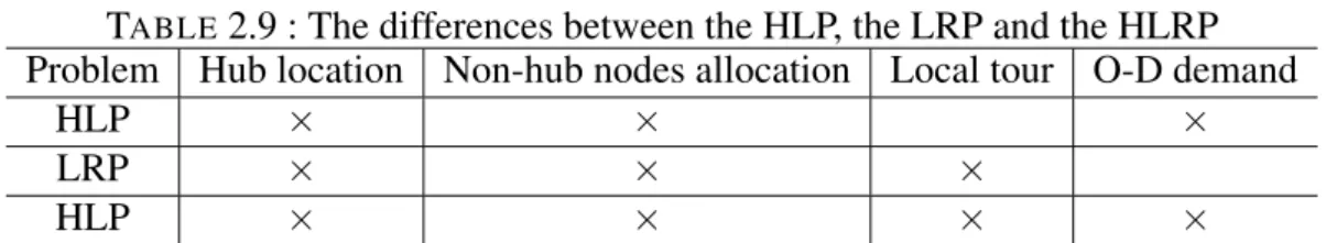
2.9 The differences between the HLP, the LRP and the HLRP . . . 41
2.10 Recent literature of the HLRP . . . 44
2.11 Solution method notation of the HLRP . . . 44
3.1 Notation used in the model of the HLRP . . . 51
4.1 The application of MA on the LRPs and the HLRPs . . . 57
4.2 Literatures of MA/hybrid GA on related problems . . . 58
5.1 Data structures of the HLRP . . . 70
5.2 Parameter values for hubs . . . 70
5.3 Cost parameter values for vehicles . . . 70
5.4 Description of the “MIPEmphasis" parameter . . . 71
5.5 Description of the “Probe" parameter . . . 71
5.6 Description of the “NodeSel" parameter . . . 72
5.7 Computational results with various values of the “MIPEmphasis" parameter . . . 72
5.8 Computational results with various values of the “Probe" (MIPEmphasis=2) . . . 73
5.9 Computational results with various values of the “NodeSel" (MIPEmphasis=2) . . . 74
5.10 Comparison of the CPLEX parameter settings . . . 75
5.11 Efficiency assessment of the valid inequalities . . . 76
5.12 Results of the MA up to 1000 iterations for medium instances . . . 77
5.13 Results of the MA up to 1000 iterations for large instances . . . 77
5.14 Computational tests on different ways of implementing the MA. . . 78
5.15 Computational results for small- and medium-sized instances . . . 79
5.16 Computational results of the MA for large sized instances . . . 80
5.17 The values of the performance indicators of the MA . . . 84
5.18 Sensitivity analysis on the hub fixed cost . . . 86
7.1 Parameter values for hubs . . . 108
7.2 Cost parameter values for vehicles . . . 108
7.3 Emission parameter values for vehicles (per unit flow). . . 108
7.4 Payoff table of epsilon constraint method . . . 108
7.5 The payoff table of Instance 10-10-10-10 . . . 109
8 LIST OF TABLES
7.6 The results of the AUGMECON model of Instance 10-10-10-10 . . . 109
7.7 The number of non-dominated solutions after each 100 iterations of the MA . . . 110
7.8 The number of “extreme solutions” dominating the solutions of the single-objective model 114 7.9 The number of “extreme solutions” dominating the solutions of the single-objective MA . 115 7.10 Results of the small instances by the bi-objective MA . . . 115
7.11 Results of the medium instances by the bi-objective MA . . . 116
7.12 Results of the large instances by the bi-objective MA . . . 117
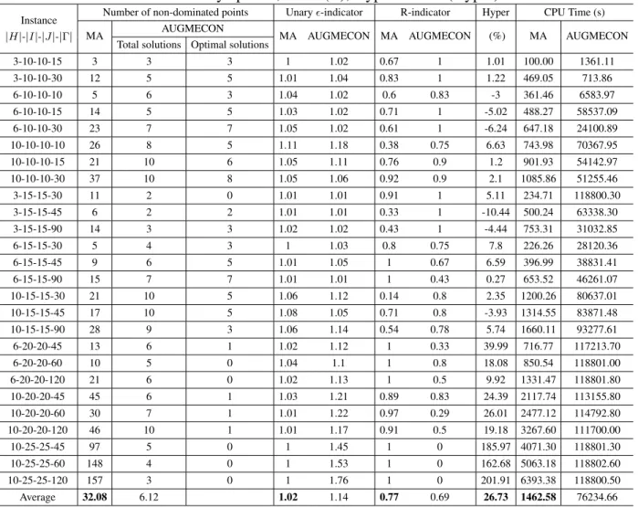
7.13 Values of unary epsilon, Ratio (R), Hypervolume (Hyper) and CPU Time . . . 119
7.14 Results comparison between the single-objective model of minimizing cost and the bi-objective MA (small instances) . . . 120
7.15 Results comparison between the single-objective model of minimizing cost and the bi-objective MA (medium instances) . . . 121
7.16 Results comparison between the single-objective model of minimizing CO2 and the bi-objective MA (small instances) . . . 121
7.17 Results comparison between the single-objective model of minimizing CO2 and the bi-objective MA (medium instances) . . . 122
7.18 Results comparison between the single-objective MA of minimizing cost and the bi-objective MA (small and medium instances) . . . 123
7.19 Results comparison between the single-objective MA of minimizing cost and the bi-objective MA (large instances) . . . 124
7.20 Results comparison between the single-objective MA of minimizing CO2and the bi-objective MA (small and medium instances) . . . 125
7.21 Results comparison between the single-objective MA of minimizing CO2and the bi-objective MA (large instances) . . . 126
9.1 Data structures for computational experiments . . . 140
9.2 CPLEX results of the first phase (HLP) . . . 141
9.3 CPLEX results of the collection VRP . . . 142
9.4 CPLEX results of the delivery VRP . . . 143
9.5 General CPLEX results of the second phase (VRP) . . . 144
9.6 Results comparison between the global model of the HLRP and the two-phase model . . . 144
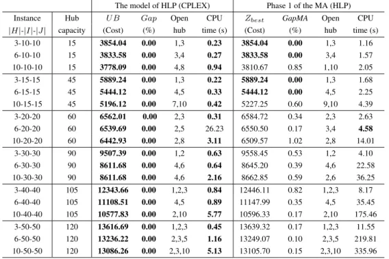
9.7 Results comparison between the model and the MA of the first phase (HLP) . . . 145
9.8 Results comparison between the model and the MA of the second phase (VRP) . . . 146
9.9 Results comparison between the two-phase model and the two-phase MA . . . 146
List of Figures
2.1 Illustration of the related problem networks . . . 42
3.1 General network of the HLRP . . . 50
4.1 Generic framework of the MA . . . 58
4.2 Representation of an HLRP solution . . . 60
4.3 Generation of an initial population . . . 61
4.4 The crossover operator . . . 65
4.5 Illustration of the mutation . . . 65
4.6 Local search on the routing . . . 66
4.7 Local search on the hub location and allocation . . . 67
5.1 Average results of the MA in 10 runs up to 1000 iterations (Instance 10-40-40-75) . . . 77
5.2 Solution evolution with CPLEX and the MA . . . 81
5.3 MA results with different hub capacities (3 potential hubs) . . . 82
5.4 Solution gaps with different potential hub numbers obtained by the MA . . . 82
5.5 MA results with different potential hub numbers (small hub capacity) . . . 83
5.6 Average values of the RSD indicators of the single-objective MA . . . 85
6.1 Solution representation of the HLRP . . . 97
6.2 Generic framework of the proposed MA for the bi-objective HLRP . . . 99
6.3 The crowding-distance of solution i . . . 101
6.4 Portions of solution space for the bi-objective HLRP . . . 104
6.5 Local search on the non-dominated solutions of NDL 1 . . . 106
7.1 Computing time evolution of the bi-objective MA (Instance 10-50-50-75) . . . 111
7.2 Non-dominated solutions with different MA iterations for small instance (6-10-10-15). . . 111
7.3 Non-dominated solutions with different MA iterations for medium instance (10-25-25-45) 111 7.4 Non-dominated solutions with different MA iterations for large instance (10-50-50-75) . . 112
7.5 Illustration of the convergence of the MA after 50 iterations (Instance 10-50-50-75) . . . . 112
7.6 Generation evolution from 100 to 400 iterations of the MA (Instance 10-50-50-75) . . . . 113
7.7 Non-dominated solutions for each run of the MA (Instance 10-50-50-75) . . . 113
7.8 The hierarchical nature of the approximate Pareto Front (Instance 10-50-50-75) . . . 114
7.9 The approximate Pareto Front of instances with 80 nodes (medium hub capacity) . . . 118
8.1 Schematic illustration of building the two-phase models . . . 130
8.2 Schematic illustration of the two-phase MA . . . 134
8.3 Solution representation of the HLP . . . 135
8.4 The crossover operator of the two-phase MA . . . 136
8.5 The mutation operator of the two-phase MA . . . 136
8.6 Initial collection and delivery routes after Phase 1 . . . 137
8.7 Local searches on collection routing in phase 2 . . . 138
10 LIST OF FIGURES
Acknowledgements
I would like to gratefully acknowledge my supervisors, Prof. Nathalie Bostel, Prof. Pierre Dejax, and Prof. Marc Paquet, for their excellent guidance and encouragements. This thesis would not have been possible without the kind support, the enthusiasm, the probing questions, and the remarkable patience of them. I cannot thank them enough.
I would also like to thank Prof. Marc Sevaux, Prof. Caroline Prodhon and Prof. Mozart Menezes for serving as my committee members. Thank you for letting my defence be an enjoyable moment, and for your brilliant comments and suggestions, thanks to you.
I would specially like to thank Ka-yu Lee, Jiuchun Gao, Yuan Bian, Axel Grimault, Quentin Tonneau for sharing memorable moments with me. Thanks are also due to Prof. Nathalie Bostel for her support and encouragement.
I am forever indebted to my parents and my family for their understanding, endless patience and encou-ragement when it was most required.
Finally, this research has been financially supported by the Chinese Government Scholarship (CSC). This support is hereby gratefully acknowledged.
I
Problem presentation and state of the art
1
Introduction
1.1
Background and motivation
In supply chain management and logistics systems, the transportation costs often represent an important part. The design of transportation network offers a great potential to reduce costs, time, the environmental impacts and improve service quality. However, the planning and operation of less-than-truckload (LTL) freight transportation networks are a challenge for transportation corporates because there are many ori-gins (suppliers) and destinations (clients) with small demand to serve in the network. Direct transportation between origins-destinations would require plenty of vehicles which are often not fully loaded. In order to reduce the number of vehicles and fully use their capacity, it is an efficient option to locate one or several facilities called hubs in the network. The hubs collect, sort and consolidate the freight from many origins, then ship it to the destinations or transfer it to other hubs. The Hub Location Problem (HLP) is concer-ned with the design of a transportation network where suppliers and clients are in direct connection with a designated hub. The field of the HLP has been abundantly researched for more than thirty years with a large amount of works. These works has been classified and synthesized in the review papers ofCampbell
[1994],Klincewicz [1998],Bryan and O’kelly[1999], Klose and Drexl[2005], Alumur and Kara[2008],
Campbell and O’Kelly[2012],Farahani et al.[2013]).
As opposed to the HLP, the Hub Location and Routing Problem (HLRP) corresponds to the design of a hub network system where the collection of goods from suppliers to a given hub and the distribution of goods from a destination hub to clients are organized through vehicle routing. The HLRP encompasses both the strategic and operational decision levels. From a total cost perspective, it includes the strategies of deciding the number of hubs to open and their location. At the operational decision level, it determines the assignment of origins and destinations to the open hubs, the flow transfer between hubs and planning of the pick-up/delivery routes. In the transport of freight, the collection and distribution of goods may be organized separately through distinct collection and delivery routes, or jointly, such as it is the case for postal services. The research on the problem of the hub location-routing is limited. Considering the wide range of applications of this problem offers many opportunities for research.
Recently, the concerns about the environmental impact on freight transport and goods operations have been mounting. It is predicted that over 80 % of the transport companies will be significantly influenced by the global warming, especially the CO2emissions, by the year of 2020 (Piecyk and McKinnon[2010]). Such
fact indicates the importance of incorporating environmental factors into the logistics-related decisions. The emissions of GHG (Green House Gas) have already been considered in areas such as the Pollution Routing Problem (PRP) (Barth et al.[2005],Xiao et al.[2012],Demir et al.[2012],Demir et al.[2014] andKramer
16 CHAPITRE 1. INTRODUCTION
et al.[2015]). In the field of the HLRP, only the work of Mohammadi et al. [2013c] has introduced the environmental effects into the HLRP in the form of a multi-objective mixed integer linear programming model.
1.2
Thesis objectives
In this thesis, we consider the Capacitated Single Allocation Hub Location-Routing problem (CSAHLRP) with independent collection and delivery processes. We seek to address the hub location and vehicle routing strategies such that the location of hubs, the allocation of supplier/client nodes to hubs, the routings between nodes allocated to the same hub, as well as the inter-hub freight transportations, in order to achieve an efficient network design system.
The first objective of the thesis is to optimize the total network cost of the HLRP. To reach this ob-jective, we propose a mixed integer linear programming model (MILP) for the CSAHLRP with aims at minimizing the total cost for the less-than-truck load (LTL) transport network. Computational experimenta-tions are conducted with CPLEX solver on the basis of a set of instances of different sizes and characteristics which we have generated. Furthermore, we propose and experiment a memetic algorithm to solve large-size CSAHLRPs.
The second objective is to study and balance the relationship of cost and environmental effect of trans-port. We extend the single-objective HLRP model into a bi-objective MILP model for minimizing the total cost and CO2 emissions. Experiments on small instances are conducted with CPLEX by means of the
epsi-lon constraint method. To solve the bi-objective CSAHLRP, a modified memetic algorithm (MA) combined with a fast elitist non-dominated sorting genetic algorithm (NSGAII) and an efficient non-domination level update (ENLU) method is developed to exhibit approximations of the Pareto front.
At last, a two-step procedure is proposed to solve the single-objective HLRP based on a hub location problem (HLP) and two distinct vehicle routing problems for suppliers and clients allocated to each hub by the first step. Our single-objective MILP model is decomposed accordingly and our MA is adapted to solve the HLRP following these two steps.
A data base of instances of different sizes and characteristics has been developed in order to conduct extensive experiments for solving all these problems using the different solution techniques and validate our approaches.
1.3
Outline of the thesis
This thesis contains four parts : Part I includes a comprehensive state-of-the-art about the Hub Location Problem (HLP), the Location Routing Problem (LRP), the Hub Location-Routing Problem (HLRP) and also relevant works concerning the environmental factors and especially the consideration of CO2emissions
of transport (Chapter2). PartIIaddresses the single-objective HLRP (Chapters3and5). PartIIIis devoted to the study on the bi-objective HLRP (Chapters6and7). Finally, the two-phase method is presented and solved in PartIV(Chapters8and9).
Chapter2provides a state-of-the-art for the HLP, the LRP and the HLRP, addressing the problem defi-nitions, classifications and mathematical formulations, as well as the solution methods. Furthermore, since we extended the HLRP into a multi-objective problem with environmental considerations, related problems such as the Pollution Routing Problem (PRP) are briefly introduced. Finally, we propose a conclusion and identify several research directions.
Chapter3describes a mathematical model of the single-objective Hub-location Routing Problem. The model contains the decisions of the Capacitated Single Allocation Hub Location Problem (CSAHLP) such as the determination of hub numbers, the decisions of hub location and flows exchange between hub points. It also integrates advanced vehicle routing formulations and decision variables, such as flow variable on vehicle, to schedule local tours for the HLRP.
1.3. OUTLINE OF THE THESIS 17
Chapter 4 proposes a Memetic Algorithm (MA) for the single-objective HLRP, combining a genetic algorithm (GA) and an iterated local search (ILS), to determine location and routing jointly.
Chapter 5 presents in detail the computational experiments which we performed with two solution methods, solving the MILP with the CPLEX solver and the MA. The generation of data sets used for all the experiments is explained, as well as the parameters setting of the CPLEX and the MA. Then, the computational results of both methods are investigated and compared.
Chapter6investigates the impacts of CO2 emissions on transport, both for the collection and delivery
routing and for inter-hub transport, and integrated the CO2 emission formulations into the single-objective
model of the HLRP to construct a bi-objective model with aims at minimizing both cost and CO2emissions.
Furthermore, to solve the bi-objective CSAHLRP, a memetic algorithm (MA) combined with a fast elitist non-dominated sorting genetic algorithm (NSGAII) is developed.
Chapter7presents the experimental results of the proposed bi-objective MA, which are compared with the results of the single-objective MA and solving the bi-objective MILP model with Epsilon Constraint (EC) method.
Chapter 8 proposes a two-phase method to solve the single-objective HLRP where the hub location and routes planing are considered sequentially in two phases. Adapted MILP models are proposed and the single-objective MA is adapted to solve the problems.
Chapter9analyzes the experimental results obtained by the two-phase MILPs solved with CPLEX and by the MA, and compares the results with the global single-objective HLRP models.
Finally, an overview of the main contributions of the thesis is summarized and some future research directions are proposed in Chapter10.
2
Literature review
Our researched Hub Location-Routing Problem (HLRP) can be considered as an integrated problem of the Hub Location Problem (HLP) and the Vehicle Routing Problem (VRP). It is also similar to the Many-to-Many Location-Routing Problem (MMLRP) which is a variant of the Location-Routing Problem (LRP). Thus it is necessary to give an overview of the two main close problems of the HLP and the LRP before researching the HLRP. This chapter provides the state-of-the-art for the HLP, the LRP and the HLRP in Sections2.1,2.2and2.3, addressing the problem definitions, classifications and mathematical formulations, as well as the solution methods. Furthermore, since we extended the HLRP into a multi-objective problem with environmental considerations, the related problems such as the Pollution Routing Problem (PRP) and the sustainable Supply Chain Network Design (SCND) are briefly introduced in Section2.4. Finally, we make a conclusion and suggest several future research proposals in Section2.5.
2.1
The Hub Location Problem
The Hub Location Problem (HLP) tackles the location of hub facilities and the assignment of customers to the hubs in the hub networks where the cost required for establishing hubs and transferring flows bet-ween hubs is lower than the cost required for transporting flows directly. The main features of the HLP (Campbell and O’Kelly [2012]) are : first, the demand is presented as the flows between the origin and destination (O-D) pairs instead of individual demands ; second, the flows transported via inter-hub benefit from a discounted cost ; last, the locations of the hubs and the allocation scheme are to be determined. The HLPs are a challenging topic since most of the problems are NP-hard even if the locations of the hubs are known (Alumur and Kara[2008]). The HLPs have been applied mainly to airlines and airport industries, postal delivery systems, supply chain management, freight transportations, telecommunication services and emergency services. More real-life applications of the HLPs can be found inFarahani et al.[2013].
The HLP and its variants have been widely researched since 1987 and several reviews have provided a comprehensive understanding in terms of fundamental definitions, classifications, hub network topologies, mathematical models, solution methods, uncertainty and competition, and so on.Campbell[1994] gave the first survey on the discrete HLPs.Klincewicz[1998] focused on the telecommunication industry and revie-wed the facility location problem in the backbone/tributary network.Bryan and O’kelly [1999] reviewed the Hub-and-Spoke (HS) networks in air transportation.Klose and Drexl[2005] provided a review of the facility location models for distribution system, especially the continuous location models and the network location models. Alumur and Kara [2008] classified the network hub location models and gave a review of the HLPs from the year of 1987 to 2007. In the article ofCampbell and O’Kelly[2012], the origins of
20 CHAPITRE 2. LITERATURE REVIEW
the hub location especially in transportation were reflected and the research of the hub location problem for 25 years were presented. They provided an insight into recent research, discussing the shortages and promising directions. Farahani et al.[2013] highlighted the research works that are published after 2007 and summarized the new recent trend of the HLPs to take into account in the future.
In this section, we provide the main criteria for classifying the HLPs. Then some fundamental and important mathematical models are presented describing various types of the HLPs. Finally, the articles of the HLPs after the year 2012 are reviewed as a supplementary of the previously published survey papers.
2.1.1
Classification of the HLPs
In order to classify the hub location problems, various criteria can be used. One of the main classifying criteria is the way of determining the hub number. When the number of hubs to open is pre-specified, the problem is called the p-HLPs, and extremely, if just one hub is established, the problem is defined as the single-Hub Location Problems (single-HLPs). On the other hand, there are problems where the number of open hubs has to be determined as part of the solution. The second important criterion is based on the allocation schemes : the single allocation scheme in which each non-hub node must be allocated to only one selected hub node ; the multiple allocation where the non-hub nodes are allowed to be assigned to more than one hub. Recently, a r–allocation HLP was proposed (Yaman [2011], Todosijevi´c et al.[2017]), allowing each non-hub node to be allocated to at most r hubs. Another important criterion takes the center and median objectives into account. The problem seeking to minimize total transportation cost (mini-sum) is the hub median problem while the problem with the objective of minimizing the maximal distance between a hub and the non-hub nodes (mini-max) is named the hub center problem. All the commonly used criteria are given as follows :
– The domain of candidate hub nodes : the discrete domain where the hubs are predetermined nodes ; the continuous domain where the solution domain is a sphere or plane ; the network where the candidate hub can be located at all the nodes of the network ;
– The certainty of the environment : the deterministic problem in which all the parameters are known ; the non-deterministic problem in which at least one parameter (such as travel time or customer de-mand) is stochastic ;
– The number of hub nodes to be located : pre-specified or not ;
– The allocation scheme : single allocation and multiple allocation ;
– The objective : center objective (mini-max) and median objective (mini-sum) ;
– The hub capacity : uncapacitated and capacitated ;
– The cost of locating hub nodes : fixed cost and no cost ;
– The cost of transportation between non-hub nodes and hub nodes : fixed cost, variable cost and no cost ;
There are also some other hub location problems such as : the dynamic HLP, including multiple time periods with various costs and adding new demand of O-D pairs in each time period (Correia et al.[2011]) ; the competitive HLP, considering the competition between multiple service providers (Niknamfar et al.
[2017]) ; and the HLPs with reliability considerations (Parvaresh et al.[2013],An et al.[2015],Azizi et al.
2.1. THE HUB LOCATION PROBLEM 21
2.1.2
Mathematical models of the HLPs
Single-Hub Location Problem
The first mathematical formulation in the research field of the HLP was proposed by O’kelly[1987b]. It dealt with an Uncapacitated Single Allocation Hub Median Location Problem in the network domain. In this problem, the number of open hubs is specified as only one (Single-HLP). No establishing cost of the hub facility is considered. Cik stands for the unit transportation cost between node i and hub k. Oi and Di
are the outgoing and ingoing flows from node i. The binary decision variable Yik is equal to 1 if node i is
allocated to a hub located at node k, 0 otherwise. Ykkequals to 1 means that the location of k is a hub node.
The single-HLP is formulated as follows :
minX i X k CikYik(Oi+ Di) (2.1) Subject to X k Ykk = 1 (2.2) X k Yik = 1 ∀i (2.3) Yik ≤ Ykk ∀i, k (2.4) Yik ∈ {0, 1} ∀i, k (2.5)
The objective function (2.1) minimizes the total transferring cost via the hub. Constraints (2.2) indicate that there is only one hub in the network. Constraints (2.3) are the allocation constraints of the non-hub nodes. Constraints (2.4) ensure that non-hub nodes can only be connected to the hub node. Constraints (2.5) define the decision variables.
Single Allocation p-Hub Median Location Problem
The model of the Single Allocation p-hub Location Problem (SApHLP) is presented as an extension of the single-HLP ofO’kelly[1987b]. Here, the SApHLP is formulated as a quadratic integer model. The number of hubs to be located in the model is denoted by p. The demand between two non-hub nodes should be transferred through at least one and at most two hub nodes. The non-hub nodes are allocated to only one hub (single allocation). In addition, a discount parameter α (0 ≤ α < 1) denotes the economies of scale due to the inter-hub transfer. Wij is the amount of flow between two nodes i and j. The SApHLP is formulated
as follows : X i X k CikYik( X j Wij) + X k X i CkiYik( X j Wji) + αX i X j X k X m WijCkmYikYjm (2.6)
22 CHAPITRE 2. LITERATURE REVIEW Subject to X k Yik = 1 ∀i (2.7) X k Ykk = p (2.8) Yik ≤ Ykk ∀i, k (2.9) Yik ∈ {0, 1} ∀i, k (2.10)
Regarding the objective function (2.6), it minimizes the total transportation cost in the hub network. The first term stands for the transportation cost from non-hub node i to hub node k if node i is allocated to hub k. The second term stands for the transportation cost from hub node k to non-hub node i if node i is allocated to hub k. Moreover, the third term of the objective function calculates the transferring cost between two hubs k and m with a discount factor. Constraints (2.7) ensure the single allocation. Constraints (2.8) stipulate that exactly p hub nodes are selected. Constraints (2.9) enforce node i be allocated to a location k only if a hub is located at node k. Finally, Constraints (2.10) define the binary decision variables.
Multiple allocation p-Hub Median Location Problem
Campbell[1991] proposed a linear mathematical formulation for the p-hub median location problem. This problem is a multiple allocation problem in which every non-hub node could be allocated to more than one hub. Cijkm is defined as the unit transportation cost starting from non-hub node i, transferring between hub nodes k and m and ending at non-hub node j (Formulation (2.11)).
Cijkm = Cik+ αCkm+ Cmj (2.11)
The non-negative allocation variables are denoted as Xijkm (Xijkm ≥ 0). Furthermore, the binary decision variables Yk equal to 1 when a hub is located at node k, otherwise 0. The other assumptions are similar
to the p-HLPs. The Multiple Allocation p-Hub Median Location Problem (MApHMLP) is formulated as follows : minX i X j X k X m CijkmWijXijkm (2.12) Subject to X k Yk = p (2.13) X k X m Xijkm = 1 ∀i, j (2.14) Xijkm ≤ Ym ∀i, j, k, m (2.15) Xijkm ≤ Yk ∀i, j, k, m (2.16) Xijkm ≥ 0 ∀i, j, k, m (2.17) Yk ∈ {0, 1} ∀k (2.18)
The objective function (2.12) minimizes the total transportation cost. Constraint (2.13) ensure that exactly p hubs should be located. Constraints (2.14) indicate that each O–D pair (i, j) is allocated to the hub nodes k and m. Constraints (2.15) and (2.16) ensure the consistency between variables Xijkm and Yk. Constraints
(2.17) and (2.18) define the decision variable types.
2.1. THE HUB LOCATION PROBLEM 23
fixed link cost gik to connect the non-hub nodes to the hub nodes. The binary variables Zik equal to 1 if a
link between the non-hub node i and the hub node k is built. The cost term (objective function) is provided below : X i X k gikZik (2.19)
The constraints are similar to the MApHMLP (Constraints (2.13) to (2.18)). Besides, the model also introduces the capacity of hubs to limit the flows allocated to each hub. That is, the flows going through each hub must fit the capacity of the hub. The capacity of the hub k is denoted as hk. The constraints (2.20)
should be considered in the p-hub median location problem : X m X i X j WijXijkm+ X s X i X j WijXijsk ≤ hkYk ∀k (2.20)
In Constraints (2.20), the first and second terms represent the total incoming and outgoing flows for the hub k.
Continuous p-Hub Location Problem
In the continuous p-HLPs, hub nodes are located based on a plane or a sphere (O’kelly[1986],Aykin and Brown[1992]) and each non-hub node must be allocated to exactly one hub (single allocation). The p hub nodes to be located are fully interconnected. The objective of the model is to minimize the total cost. At least one and at most two hub nodes should be visited for transferring flows of each O-D pair. The hubs are uncapacitated and no fixed establishing hub cost is considered.
The notation of the problem is similar to the SApHMLPs. Moreover, a vector Ni stands for the location
vector of non-hub node i ; the decision variable Pk denotes the location vector of hub node k (k =1, ...,
p) ; d(i, j) is considered as the Euclidean distance between two nodes i and j. The continuous p-HLP is formulated as follows : minX i X j X k X m WijYikYjm(d(Ni, Pk) + αd(Pk, Pm) + d(Nj, Pm)) (2.21) Subject to X k Yik = 1 ∀i (2.22) Pk = (ak, bk) k = 1, ..., p (2.23) Yij ∈ {0, 1} ∀i, j (2.24)
The objective function (2.21) minimizes the total transportation cost in the hub network. The first term is the transportation cost originated from the non-hub node i to the hub node k, and the second term is the transportation cost between hub nodes, finally the third term is the transportation cost generated from the hub node k to the non-hub node m. Constraints (2.22) indicate the single allocation. Constraints (2.23) and (2.24) define the decision variables.
p-Hub Center Location Problem
The p-Hub Center Location Problem aims to minimize the maximum distance (cost) of origin-destination (O-D) pairs. The real-life applications of this problem exist in the emergency facility location problem and the perishable commodities transportation problem (Campbell[1994]). Note that the constraints and notation of the problem are similar to the MApHMLPs (constraints (2.13) to (2.18)) except for the objective
24 CHAPITRE 2. LITERATURE REVIEW
function which is formulated as follows :
min max
i,j,k,mC km
ij WijXijkm (2.25)
The objective function (2.25) minimizes the maximum transportation cost of O-D pairs. For other improved models of the p-Hub Center Location Problems, the articles ofKara and Tansel[2000],Yaman and Elloumi
[2012],Campbell et al.[2007] andErnst et al.[2009] are recommended.
Hub Covering Location Problems
The classic Hub Covering Location Problem seeks to find the best locations for hubs so as to ensure each O-D pair is covered by a pair of hub nodes (Campbell[1994]). Each O-D pair is covered if the cost (time, etc.) is lower than or equal to a pre-specified value of γij (Constraint (2.26)).
Cijkm ≤ γij (2.26)
The Hub Covering Location Problem can be further developed into three other variants : the p-Hub Covering Location Problem, the Hub Set Covering Location Problem and the p-Hub Maximal Covering Location Problems.
Regarding the p-Hub Covering Location Problem, the only difference compared to the classic ones is the pre-specified number of open hubs.
The Hub Set Covering Location Problem deals with the selection of open hubs which are subjected to a fixed establishing cost, and the allocations of O-D pairs to the hubs. The notation of the problem is given as : Fkis the fixed cost of selecting node k as a hub ; Cijkm is the transfer cost from the origin node i to the
destination node j via hubs located at nodes k and m ; γij stands for the maximum cost allowed for covering
links connecting the nodes i and j ; Yk is the location variable and Vijkm is equal to 1 if the hubs k and m
cover the O-D pair (i, j), otherwise 0. The Hub Set Covering Location Problem is formulated as follows :
minX k FkYk (2.27) Subject to X k X m VijkmXijkm ≥ 1 ∀i, j (2.28) Xijkm ≤ Ym ∀i, j, k, m (2.29) Xijkm ≤ Yk ∀i, j, k, m (2.30) Xijkm ≥ 0 ∀k (2.31) Yk ∈ {0, 1} ∀k (2.32)
The objective of the model is to minimize the total cost of opening new hubs (Formula (2.27)). Constraints (2.28) impose that an O-D pair is covered by at least one hub pair. Constraints (2.29) and (2.30) ensure that the origin node i and destination node j can only be allocated to the nodes of k and m that are selected as hubs. Constraints (2.31) and (2.32) define the decision variables.
The p-Hub Maximal Covering Location Problems is devoted to locate p hubs to maximize the demands within a coverage distance. The fixed cost of opening hubs is not considered in the model. This problem is formulated as follows : max X i X j X k X m WijVijkmX km ij (2.33)
2.1. THE HUB LOCATION PROBLEM 25
The objective function (2.33) maximizes the amount of transportation demand covered. The constraints are the same as in the MApHMLP from (2.15) to (2.18).
Multi-objective p-Hub Location Problem
The cost and service, as well as sustainable considerations, are of great importance in hub networks de-signing. The services regarded in many articles include the service time (da Graça Costa et al. [2008]), the travel time (Mohammadi et al. [2013a], Ebrahimi Zade and Lotfi[2015], Yang et al. [2017]) and the responsiveness and social aspects (Zhalechian et al.[2017a]). The environment aspects in literature mainly include the pollution gas such as CO2emissions (Mohammadi et al.[2014],Ghodratnama et al.[2015]).
The multi-objective HLP model presented was proposed by da Graça Costa et al. [2008] with two objectives : minimizing the transportation cost and the maximum service time of the hub nodes. It is an uncapacitated single allocation p-HLP and the hub nodes are fully connected. At least one and at most two hub nodes should be visited for transferring flows between two non-hub nodes. There is no fixed cost to initiate service at hub nodes. A new notation of Tkis introduced which stands for the operating time of hub
k to process one unit flow. The multi-objective HLP is formulated as follows :
min X i X j X k X m WijYikYjm(Cik+ αCkm+ Cjm) (2.34) min max k {Tk( X i X j WijYik+ X i X j WjiYjmYik)} (2.35)
The first objective function (2.34) minimizes the total transportation cost in the hub network. The second objective function (2.35) minimizes the maximum service time of hub nodes. The constraints are the same as in the SApHMLP (Constraints (2.7) to (2.10)).
Capacitated Single Allocation Hub Location Problem
Regarding the models of the Capacitated Single Allocation Hub Location Problem (CSAHLP),Ernst and Krishnamoorthy[1999] provided an integer linear formulation with an inter-hub flow fraction variable and an allocation variable.Correia et al.[2011] considered the hub capacity as another decision variable with varied fixed installing costs corresponding to relevant hub capacity. They proposed several mixed integer formulations and a set of preprocessing tests to reduce the formulation size.Saiedy et al.[2011] presented an improved model of CSAHLP with n-hub centers with less indices and constraints to get the model faster to solve by CPLEX for small and medium instances.Karimi et al.[2014] imposed the hub capacity constraint on the single hierarchical hub median location problem and studied the effect of hub capacity on total costs based on the Iranian Airport Data (IAD).
Here, we describe the model proposed byErnst and Krishnamoorthy[1999]. Assume that in the postal delivery network, mail from postal districts (nodes in the network) has to be collected by a mail sorting center (hub in the network) with a limited sorting ability (hub capacity). The model deals with the number and location of hubs and allocations of non-hub nodes to hubs in order to minimize the total network cost.
The CSAHLP in a postal delivery network is defined on a complete graph G = (N, A) in which N is the set of n nodes and A is the set of arcs. The decision variable zik ∈ {0, 1} equals to 1 if the non-hub node i is
allocated to a hub k, and 0 otherwise. If one hub is located at node k, zkk= 1, otherwise 0. Another decision
variable Ykli is defined as the total amount of commodity flows from the non-hub i transferred between the hubs k and l. Further, α, β and γ are denoted as the unit transporting cost of inter-hub transfers, pick-ups and deliveries, respectively. Oi =
P
j∈N qij and Di =
P
j∈Nqji represent the demand of the pick-up and
the delivery of the node i. dij is the distance from node i to node j. Γk is the capacity of hub k. The fixed
26 CHAPITRE 2. LITERATURE REVIEW min X i∈N X k∈N dikzik(βOi+ γDi) + X i∈N X k∈N X l∈N αdklYkli + X k∈N Fkzkk (2.36) Subject to X k∈N zik = 1 ∀i ∈ N (2.37) zik ≤ zkk ∀i, k ∈ N (2.38) X i∈N Oizik ≤ Γkzkk ∀k ∈ N (2.39) X l∈N Ykli −X l∈N Ylki = Oizik− X j∈N qijzjk ∀i, k ∈ N (2.40) zik ∈ {0, 1} ∀i, k ∈ N (2.41) Ykli ≥ 0 ∀i, k ∈ N (2.42)
Objective function (2.36) minimizes the collection and delivery cost, the inter-hub transportation cost and the fixed cost of locating hubs. Constraints (2.37) are the single allocation constraint. Constraints (2.38) ensure that the non-hub nodes are allocated to a hub only if it is open. Constraints (2.39) limit total collection demand on each hub. Constraints (2.40) inquire that the supply at the nodes is determined by the allocations zik. Constraints (2.41) and (2.42) specify the decision variables.
2.1.3
Data sets of the HLPs
In the hub location research, two data sets are commonly used : the AP (Australian Post) data set and the CAB (U.S. Civil Aeronautics Board) data set. They provide valuable benchmarks derived from real-world applications of various scales and have been applied in most of the hub location literature. The CAB data set is based on the airline passenger traffic between 25 US cities in 1970 and was first introduced for hub location inO’kelly [1987b]. The AP data set (Ernst and Krishnamoorthy [1996]) is derived from the Australian postal delivery network with up to 200 nodes of postal districts in Sydney, Australia. The flow matrix of the CAB is symmetrical while the flow matrix of the AP is not. Another data set used in the literature is the Turkey postal (PTT) data set for ground transportation between 81 cities in Turkey. This data set was introduced inTan and Kara[2007] to dealt with the latest arrival hub covering problem, minimizing the number of hubs within a predetermined time bound.Meyer et al.[2009] created random instances with up to 400 nodes which are called URAND data sets for the single allocation p-hub center problem. Based on the AP data set with 200 nodes, Silva and Cunha[2009] generated four larger instances with 300 and 400 nodes and applied reduction factors (0.9 and 0.8) to the fixed costs of hubs. Table2.1shows the details of the data sets and the first reference in the field of the HLP.
TABLE2.1 : Data sets of the HLPs
Acronym First reference Maximum number Size1 Parameter2 Resource
of nodes
CAB O’kelly[1987b] 25 2-4/10-25 α={0.2, 0.4, 0.6, 0.8, 1.0} U.S. airline β = γ =1 passenger traffic AP Ernst and Krishnamoorthy[1996] 200 2-20/10-200 α =0.75, β =3 Australian postal γ =2 delivery network PTT Tan and Kara[2007] 81 - α0={0.2, 0.4, 0.6, 0.8, 1.0} Turky national postal
service (PTT) URAND Meyer et al.[2009] 400 2-5/100-400 α =0.75 Random
Silva Silva and Cunha[2009] 400 2-5/300-400 α =0.75, β =3 Based on AP data set γ =2 with 200 nodes
1Structure of the instance size : min–max number of facilities/ min–max number of customers
2.1. THE HUB LOCATION PROBLEM 27
2.1.4
State-of-the-art of the HLPs in recent five years
In this part, the main research of the HLPs covering the period from 2013 to 2017 are reviewed as a com-plementary of the previous survey articles.
(1) Uncapacitated HLPs
It is seemed that the uncapacitated HLPs are the main focus in the field of HLPs in recent years.Mari´c et al. [2013] designed a Memetic Algorithm (MA) with two local search heuristics for solving the Un-capacitated Single Allocation Hub Location Problem (USAHLP). The experimental results based on the Civil Aeronautics Board and Australian Postal (CAB/AP) data sets (Ernst and Krishnamoorthy [1999]) showed the superiority of the proposed MA over existing heuristic approaches for solving the USAHLP.
Abyazi-Sani and Ghanbari [2016] proposed an efficient Tabu search (TS) with several new tabu rules for the USAHLP. The computational experiments were conducted on all the CAB/AP data sets and also the data set with 300 and 400 nodes created by Silva and Cunha [2009]. Compared with recently proposed approaches, the results showed that the proposed TS was able to find all the optimal and best benchmark solutions. More importantly, it also decreased the computational time.
Kratica[2013] dealt with the Uncapacitated Multiple Allocation p-hub Median Problem (UMApHMLP) by an Electromagnetism-like method (EM). The EM was able to find excellent results on large-scale ins-tances of the standard AP data set with up to 200 nodes and the insins-tances with up to 400 nodes which was created by Meyer et al. [2009]. Later, they extended this method to solve the capacitated version of the problem.Bailey et al.[2013] proposed a new solution method based on a Particle Swarm Optimization (PSO) to solve the UMApHMLP. To solve the Uncapacitated Single Allocation p-Hub Location Problem (USApHLP),Rasoulinejad et al.[2013] introduced a Tabu Search (TS) and applied a clustering method to improve the performance of the TS. Recently,Meier[2017] introduced the integer variables for the number of used vehicles into the Uncapacitated Single Allocation p-Hub Median Location Problem (USApHMLP). A mixed integer program formulation with fewer variables but more constraints were proposed to form a more precise model for the problem.
Regarding the Uncapacitated Hub Location Covering Problem, Peker and Kara [2015] extended the definition of coverage and introduced “partial coverage” which changes with distance. They studied the “partial converge” of the single and multiple p-Hub Maximal Covering Problem by relaxing the definition of the binary coverage. The p-Hub Maximal Covering Problem aims to locate p hubs within a coverage distance so as to maximize the demands.Silva and Cunha[2017] developed a TS heuristic for the Uncapa-citated Single Allocation p-Hub Maximal Covering Problem to solve to optimality the instances with up to 50 nodes from the AP data set. Furthermore, the proposed TS was also able to solve all instances of the AP data set with up to 200 nodes in shorter CPU times.Ebrahimi-Zade et al.[2016] proposed a dynamic model with flexible covering radius for the multi-period Hub Set Covering Problem and solved it by a modified Genetic Algorithm (GA) based on a real-world case study.
Damgacioglu et al.[2015] coped with the uncapacitated single allocation Planar Hub Location Problem (PHLP) in which the solution domain of the problem is a plane. A mathematical formulation was proposed for the PHLP and a Genetic Algorithm (PHLGA) was developed to solve the problem.
(2) Capacitated HLPs
Compared to its uncapacitated version, capacitated HLPs were not so extensively studied.Correia et al.
[2014] considered the multiple products transportation of the capacitated single-allocation hub location problem (CSAHLP). Two cases were considered : (1) the hubs can handle only one product or (2) the hubs can handle all the types of products. Later, Stanojevi´c et al. [2015] proposed a hybrid optimization method, consisting of an Evolutionary Algorithm (EA) and a Branch-and-Bound (B& B) method to solve the CSAHLP and tested it on the standard Australia Post (AP) hub data sets with up to 300 nodes.
(3) Variant HLPs
Some researches extend the HLPs with more realistic variants in the real-world such as the unpredictable hub disruptions (Parvaresh et al.[2013],An et al.[2015],Azizi et al.[2016]), the multiple products (Correia et al.[2014]), the multimodal hubs (SteadieSeifi et al.[2014], Serper and Alumur[2016]), the hubs which are not fully linked (Martins de Sá et al.[2015a],Martins de Sá et al.[2015b]), the serving orders (Puerto
28 CHAPITRE 2. LITERATURE REVIEW
et al.[2011],Puerto et al.[2013])) and so on.
One of the interest of the variant HLPs in recent years is the HLP with unpredictable hub disruptions. This problem considers the hub disruptions which may be caused by natural disasters, labour dispute and weather conditions. Parvaresh et al.[2013] formulated a bi-level game model for the Multiple Allocation p-Hub Median Problem under intentional disruptions. Two algorithms based on the Simulated Annealing (SA) were defined to solve the problem.An et al.[2015] proposed a set of reliable Hub-and-Spoke (H&S) network design models for both single and multiple allocation schemes considering disruptions and alterna-tive routes. A Lagrangian relaxation (LR) algorithm with variable fixing and a Branch-and-Bound (B&B) method was implemented to solve the CAB instances.Azizi et al. [2016] assumed that if a hub was dis-rupted, the entire demand initially served by this hub was handled by a backup facility. They proposed a mathematical formulation to minimize the regular and hub fail transportation cost. A genetic algorithm (GA) was implemented to test large instances of the CAB and Turkish Postal System.
Saboury et al.[2013] proposed an advanced mathematical programming formulation for a specific ap-plication of the HLP, namely the Hub Location Problem with fully interconnected backbone and access networks. Two hybrid heuristics incorporating a Variable Neighborhood Search (VNS) into the SA and TS were developed to obtain the optimal solutions of 24 small instances from the literature. Furthermore, some newly generated medium and large instances were solved efficiently in a quite short CPU time.
In the articles ofMartins de Sá et al.[2015a]a andMartins de Sá et al.[2015b]b, a hub network where not all the hub facilities were fully interconnected was considered. The problem was called the Hub Line Location Problem (HLLP) in which the locations of all the selected hubs were linked together by means of a path or a line. The problem coped with the minimization of the total travel time for O-P pairs. A Benders-Branch-and-Cut algorithm and several heuristic algorithms are applied to solve the problem.
Puerto et al.[2016] focused on the Capacitated Single Allocation Ordered Median Hub Location pro-blem (CSA-OMHLP) which was originally fromPuerto et al.[2011] andPuerto et al.[2013]. The Ordered Median Hub Location problem introduced the ordinal information by applying rank dependent compen-sation factors on routings from the origin nodes to the hubs. They presented a new formulation with two preprocessing phases and a Branch-and-Bound-and-Cut (B&B&Cut) based algorithm to solve the model. The tests on AP data set proved that the proposed method gave good solutions in competitive running times.
Serper and Alumur [2016] considered the intermodal hub networks by introducing alternative trans-portation modes and vehicle types. Furthermore, they incorporated decisions on designing the inter-hub network that the hubs are not fully interconnected. A variable neighbourhood search algorithm was develo-ped and tested on the Turkish network and CAB data sets. Such study is seemed to be so far the first hub location study in the literature determining the optimal number of various types of vehicles to operate the intermodal hub network.
(3) The HLPs with uncertainty
Recently, there is a new trend in the research of the HLPs taking into account the presence of uncertainty. Uncertainty can be regarded as an unforeseen and unpredictable situations of a system due to the flaws of human knowledge (Guzmáan et al.[2016]). The uncertainty in the hub networks may occur in flows, costs, times and hub operations.
Yang et al.[2013b] presented a p-Hub Center Problem with fuzzy travel times. They adopted the Value-at-Risk (VaR) criterion in the formulation and developed a hybrid algorithm of Genetic Algorithm (GA) and local search. The numerical experiments showed that the proposed algorithm outperformed the LINGO sol-ver and the standard GA.Mohammadi et al.[2016] studied a bi-objective Single Allocation p-Hub Center-Median Problem (BSpHCMP) and assumed that the flows, costs, times and hub operations were under uncertainty. A fuzzy-queuing approach was used to model the uncertainties and an Evolutionary Algorithm (EA) based on game theory and Invasive Weed Optimization (IWO) algorithm was developed. The overview of the literature on the fuzzy models and resolution methods was given byGuzmáan et al.[2016].
Talbi and Todosijevi´c [2017] focused on the uncertainty in the flow for the Uncapacitated Multiple Allocation p-Hub Median Problem(UMApHMP). They formulated a deterministic UMApHMP model and then introduced uncertainty into the model by assuming that the flows to be transferred are subject to
2.2. THE LOCATION-ROUTING PROBLEMS 29
uncertainty. A new robustness measure was proposed in order to build a solution which is robust for any realization of the flow. Furthermore, a Variable Neighborhood Search (VNS) was developed to evaluate the performance of the robustness measures on benchmark p-hub instances.
The studies of the HLPs are presented in Table2.3and2.4. Table2.3gives a review of the HLPs without uncertainty while Table2.4 shows the HLP references taking into account the uncertainties. To introduce various kinds of HLPs properly, The meanings of different notation are explained in Table2.2.
TABLE2.2 : Notations for different HLPs
Capacity of hubs Allocation scheme Type of HLPs Number of hubs Capacitated (C) Single allocation (SA) Median (M) Single (1) Uncapacitated (U) Multiple allocation (MA) Center (T) More than one (p)
r-allocation (RA) Covering (V) Set covering (SV) Maximum covering (MV) Line location (HLLP) Order Median (OM) Sustainable (SHLP)
2.1.5
Conclusion
In this section, we include a summary of the main classifications of the hub location problems. The funda-mental mathematical formulations for various hub location problems are also presented. Furthermore, we provide a concise overview of the main developments and most recent trends in hub location problems by reviewing the researches in recent five years including exact methods, heuristic and metaheuristic solution methods. The described research shows that the field of hub location is moving towards new directions in terms of considering various realistic problem variants.
2.2
The Location-routing Problems
The objective of the Location-Routing Problem (LRP) is to serve customers at minimum total cost by jointly determining the locations of candidate facilities and constructing an associated set of vehicle routes. It encompasses two NP-hard problems : the classic Facility Location Problem (FLP) and the Vehicle Routing Problem (VRP). In special cases, if all customers are served by a depot through direct transportation, the LRP becomes a standard location problem. On the other hand, if the locations of the facilities are pre-specified, the LRP reduces to a VRP (Nagy and Salhi [2007]). Wide real-life applications of the LRPs have been studied in terms of locating capacitated urban distribution centers, consumer goods distributions, postal or parcel deliveries and so on (Drexl and Schneider [2015]). For example, Menezes et al. [2016] developed an easily implementable rough-cut approach and implemented it to solve two real life cases : the supermarket chain of Casino Group in southeast France and the household material recycling network in Calgary of Canada. This methodology was based on a pragmatic transformation of the distances between the candidate locations and the demand nodes. It divided the LRP in two sub-problems : locating a collection of regional distribution centres (RDCs) to minimize the total travelled distance ; finding the optimal routes for the configuration obtained in the first stage (VRP).
The LRPs have been studied for decades since 1998 with a significant amount of literature on the general LRPs and their variant problems. Several survey papers of the LRPs have given an overview of the literature from different perspectives. It seems that Balakrishnan et al. [1987] gave the first survey on the iterated facility location and the vehicle routing problems. Other early survey papers can be found inLaporte et al.
30 CHAPITRE 2. LITERATURE REVIEW
TABLE2.3 : Reviews of the HLPs without uncertainty
Problem Article Exact solution algorithms Heuristics/metaheuristics U-RA-M-p-HLP Todosijevi´c et al.[2017] Variable Neighborhood Search U-SA-V-HLP Dukkanci and Kara[2017] Heuristic based on subgradient approach U-SA-MV-p-HLP Silva and Cunha[2017] Tabu Search
U-SA-M-p-HLP Meier[2017] MIP formulations
Mesgari and Barzinpour[2016] Variable Neighborhood Search &&Social network centrality measure U-SA-T-p-HLP Brimberg et al.[2017] Nested Variable Neighborhood
Descent Strategy U-SA-M-p-HLP Azizi et al.[2016] Genetic Algorithm U-SA-SV-HLP Ebrahimi-Zade et al.[2016] Genetic Algorithm U-SA-HLP Damgacioglu et al.[2015] Genetic Algorithm
An et al.[2015] Lagrangian relaxation && Branch-and-Bound
Saboury et al.[2013] Variable Neighborhood Search
Mari´c et al.[2013] Memetic Algorithm
Bailey et al.[2013] Particle Swarm Optimization
Rasoulinejad et al.[2013] Simulated Annealing U-SA-OM-HLP Puerto et al.[2013] Branch-and-Bound-and-Cut
U-MA-T-p-HLP Miskovic[2017] Memetic Algorithm U-MA-HLLP Martins de Sá et al.[2015b] Benders-Branch-and-Cut Heuristic algorithms U-MA-M-p-HLP Mahmutogullari and Kara[2016] Enumeration-based algorithms
Parvaresh et al.[2013] Tabu Search
Kratica[2013] Electromagnetism-like Method U-MA-HLP He et al.[2015] MIP heuristic
U-HLLP Martins de Sá et al.[2015a] Benders Decomposition Algorithm
C-SA-HLP Hoff et al.[2017] Memory structures &&Local Search
Tanash et al.[2017] Branch-and-Bound
Serper and Alumur[2016] Variable Neighborhood Search
Stanojevi´c et al.[2015] Evolutionary Algorithm && Branch-and-Bound
Niknamfar et al.[2017] Multi-objective Biogeography-based Optimization && Opposition NSGA-II C-SA-OM-HLP Puerto et al.[2016] Branch-and-Bound-and-Cut
2.2. THE LOCATION-ROUTING PROBLEMS 31
TABLE2.4 : Reviews of the HLPs with uncertainty
Single-objective HLPs
Problem Article Exact solution algorithms Heuristic /metaheuristic solution algorithms C-MA-HLP Meraklı and Yaman[2017] Benders decomposition algorithm
U-SA-T-p-HLP Gao and Qin[2016] Chance-constrained programming Intelligent algorithm
Yang et al.[2013b] Genetic Algorithm && Local search
Yang et al.[2013a] Particle Swarm Optimization U-SA-IH&S Yang et al.[2016] Fuzzy random programming Multi-start simulated annealing U-MA-M-p-HLP Meraklı and Yaman[2016] Benders decomposition algorithm
U-MA-HLP Zhai et al.[2016] Variable neighbourhood search && Genetic Algotithm U-RA-M- p-HLP Peiró et al.[2014] Heuristic based on GRASP U-HLP Shahabi and Unnikrishnan[2014] Conic integer programming
Shahabi and Unnikrishnan[2014] Conic integer programming Multi-objective HLPs
Problem Article Exact solution algorithms Heuristic /metaheuristic solution algorithms U-SA-HLP Yang et al.[2017] Two-phase approach
C-SA-HLP Zhalechian et al.[2017b] Two-phase solution method
C-SA-p-HLP Zhalechian et al.[2017c] Me-based possibilistic programming Hybrid differential evolution&& imperialist competitive algorithm U-SA-T-M-p-HLP Mohammadi et al.[2016] Fuzzy-queuing approach Evolutionary algorithm
based on game theory && invasive weed optimization C-SA-V-p-HLP Ghodratnama et al.[2015] Fuzzy goal programming
&&Torabi and Hassini’s method
Mohammadi et al.[2013a] Imperialist Competitive Algorithm C-SA-SHLP Mohammadi et al.[2014] Mixed possibilistic– Simulated annealing &&
32 CHAPITRE 2. LITERATURE REVIEW
et al. (2013)Lopes et al. [2013] presented a taxonomy taking into account the structure characteristics, solution methods and objectives of the LRPs up to 2013. Prodhon and Prins [2014] analysed the recent literature of the standard and new extensions of the LPR since the survey ofNagy and Salhi[2007]. Drexl and Schneider [2015] focused on the survey of variants and extensions of the LRP. Albareda-Sambola
[2015] provided an overview of the most relevant contributions on the so-called classical location-routing problems. Later in 2017,Schneider and Drexl[2017] reviewed the literature of standard LRP between 2006 and spring 2016 by presenting detailed descriptions of the individual articles.
In this section, we classified the LRP and its variant problems by several criteria that most of the lite-rature used in Section2.2.1. The benchmark instances are also given in Section2.2.2. In Section2.2.3, we focus on the standard Capacitated Location-routing Problem (CLRP), describing the definition of the stan-dard CLRP, the mathematical models and afterwards, the solution methods to solve the stanstan-dard CLRP are reviewed from the year of 2002 to 2017. Section2.2.4gives a breif introduction of the multi-objective LRPs and highlights the most relevant articles to our problems. Finally, the conclusion of the main constribution is in the Section2.2.5.
2.2.1
Classification of the LRPs
Since there are numerous types or variants of LRPs, a summary of the important classifying criteria helps to capture the main characteristics of the problems and get an overview of the research field of the LRPs. The basic and main criteria of the LPRs are shown below :
– The solution domain : the discrete domain where the potential locations for opening facilities are particular nodes of a graph ; the continuous domain where the facilities are allowed to be located anywhere in a sphere or plane ; the network where the candidate locations may be chosen to locate facilities at any vertex or anywhere on a link (edge, arc) of a network ;
– The nature of data : the LRPs in which all the data are pre-specified (deterministic data) ; the LRPs that some of the data are given with a probability distributions (stochastic data) ; and the LRPs that some of the data are in the form of fuzzy numbers (fuzzy data). One can refer to the survey paper of
Berman et al.[1995] regarding the LRPs with uncertainty ;
– The planning period : the static problems compromise only one determined period ; the periodic LRPs (PLRP) include multiple planning periods with deterministic data ; the dynamic LRPs also consider multiple planning periods but some information such as customer demand are unknown at first and become available over time ;
– The vertex routing and arc routing : the vertex routing problems serve customers at vertices while the Location-arc routing problems (LARP) consider demands along the arcs of the network ;
– The echelon of distribution network : in the single echelon problems, customers are directly served by depots ; in the multiple echelon problems, routes are added to supply the depots from several main facilities or plants before serving the customers. For each echelon, some pre-specified vehicles are only allowed to visit the facilities defining the echelon. There are load transfers among different echelons. In particular, many papers of the two-echelon LRPs (2E-LRP) have appeared in the last few years and one survey paper of the 2E-LRP is found given byCuda et al.[2015] ;
– The number of objective functions : single-objective problems usually consider the minimization of the total cost while multi-objective problems deal with several objective functions such as cost, service quality and environment affection ;
Other main variant LRPs are the Prize-collecting LRPs (PCLRPs), the Location-inventory-routing pro-blem, the LRP with Simultaneous Pickup and Delivery (LRPSPD) and the Many-to-many LRPs. PCLRPs
2.2. THE LOCATION-ROUTING PROBLEMS 33
allow some customers not to be visited by any tour but a penalty called outsourcing cost are applied to these customers (Ahn et al.[2012]). Location-inventory-routing problems take the inventory into account and ta-ckle with the decisions of time and amount of demand to order from the manufacturer (Zhang et al.[2008]). The LRPSPD not only consider the delivery scheme but also include the pick-up demand of customers in the network. Goods are delivered to one customer from one selected depot. At the same time, the goods are picked up from the customer. The simultaneous deliveries and pick-ups for one customer happen in the same vehicle (Karaoglan et al.[2011]). The many-to-many LRPs (MMLRPs), which is very similar to our researched problem, consider both the simultaneous or separate pick-ups and deliveries with pre-determined O-D demands. The decisions of load transfer between the facilities are also part of the solutions (Nagy and Salhi[1998]). The concrete reviews of the MMLRPs are presented in Section2.3.
Recently, a new variant of LRPs called the Latency Location-Routing Problem (LLRP) is introduced consisting of optimally determining both the locations of depots and the routes of vehicles to minimize the waiting time of recipients (Moshref-Javadi and Lee[2016]). Other variant LRPs were discussed in the article ofDrexl and Schneider[2015].
2.2.2
Benchmark instances of the LRPs
In order to evaluate the efficiency of the developed solution methods and the solution quality, some standar-dized benchmark instances have been extensively used in recent literature. The list of the main benchmark instances are show in Table2.5(Drexl and Schneider[2015],Schneider and Drexl[2017]). The benchmarks for the LRP are also widely used in many papers of LRP variants to assess the performance of their propo-sed methods. Table2.5 presents the reference which was the first to introduce the instances, the numbers and size of the instances, as well as the internet link of getting access to those instances. For simplicity, the following sections use the acronyms of the benchmark instances to discuss the articles that are mentioned.
34 CHAPITRE 2. LITERATURE REVIEW
TABLE2.5 : Benchmark instances of the LRPs
Acronym First reference Number of Size1 Link
Instances
Perl Ph.D. dissertation 5 2–15/12–318 sweet.ua.pt/sbarreto/_private of Perl (1983) /SergioBarretoHomePage.htm TB Tuzun and Burke[1999] 36 10–20/100–200 prodhonc.free.fr/homepage
B Ph.D. dissertation of Barreto (2003) 13 5–14/21–150 sweet.ua.pt/sbarreto/_private and used inBarreto et al.[2007] /SergioBarretoHomePage.htm ADF Albareda-Sambola et al.[2005] 15 5–10/10–30 Not on the Internet
PPW Prins et al.[2006b] 30 5–10/20–200 prodhonc.free.fr/homepage ABR Akca et al.[2009] 12 5/30–40 claudio.contardo.org/instances BMW Baldacci et al.[2011] 4 14/150–199 claudio.contardo.org/instances HKM Harks et al.[2013] 27 100–1000/1000–10,000
www.coga.tu-berlin.de/v-menue/download_media/clrlib 2E-LRP2
GPTV Gonzalez-Feliu et al.[2008] 105 1/2–4/12–50 people.brunel.ac.uk/ ?mastjjb /-jeb/orlib/vrp2einfo.html CPMT Crainic et al.[2010] 132 1/2–10/50–250 people.brunel.ac.uk/ ?mastjjb
/-jeb/orlib/vrp2einfo.html NPP-N Nguyen et al.[2010] 24 1/5–10/20–200 prodhonc.free.fr/homepage NPP-P Nguyen et al.[2010] (PPW modified 30 1/5–10/20–200 prodhonc.free.fr/homepage
by adding one level-0 facility)
S Sterle[2008] 93 2–5/3–20/8–200 Not on the Internet Other LRPs
Prodhon PLRP3,Prodhon and Prins[2008] 30 5–10/20–200 prodhonc.free.fr/homepage
KAKD LRPSPD4,Karaoglan et al.[2011] 37 2–10/8–100 Not on the Internet
LPFS LARP5,Lopes et al.[2014] 30 11–140 lore.web.ua.pt 1Structure of the instance size : min–max number of facilities/ min–max number of customers
22E-LRP : two echelon location-routing problem 3PLRP : periodic location-routing problem
4LRPSPD : location-routing problem with simultaneous pick-up and delivery 5LARP : location-arc routing problem