THESIS PRESENTED TO
ÉCOLE DE TECHNOLOGIE SUPÉRIEURE
IN PARTIAL FULFILLEMENT OF THE REQUIREMENTS FOR A MASTER’S DEGREE WITH THESIS IN AEROSPACE ENGINEERING
M. A. Sc.
BY Wen Yang LI
FINITE ELEMENT MODEL FOR THREE-DIMENSIONAL COMPRESSIBLE TURBULENT FLOWS
MONTREAL, OCTOBER 2ND, 2015
© Copyright
Reproduction, saving or sharing of the content of this document, in whole or in part, is prohibited. A reader who wishes to print this document or save it on any medium must first obtain the author’s permission.
BY THE FOLLOWING BOARD OF EXAMINERS
M. Azzeddine Soulaïmani, Thesis Supervisor
Mechanical Engineering Department, École de technologie supérieure
M. Amine Ben Haj Ali, Thesis Co-supervisor Advanced Aerodynamics, Bombardier Aerospace
M. François Morency, Chair, Board of Examiners
Mechanical Engineering Department, École de technologie supérieure
M. Kurt Sermeus, Aerodynamicist Advanced Aerodynamics, Bombardier
THIS THESIS WAS PRESENTED AND DEFENDED
IN THE PRESENCE OF A BOARD OF EXAMINERS AND THE PUBLIC ON JULY 17TH, 2015
I would like to thank my director Azzeddine Soulaïmani and co-director Amine Ben Haj Ali. They guided me through this wonderful academic process. They gave me a lot of advice on my research and helped me overcome countless difficulties.
I would like to thank the members of the jury for the time and effort to review my research work. I would like to thank all the professors who taught the courses I followed. The knowledge I gained in these courses inspired me a lot during my research. I would like to thank l’Ecole de Technologie Supérieure for providing me a fantastic environment and academic experience. I would like to thank the supercomputing center CLUMEQ for providing me access to their facilities.
I would also like to thank my parents for encouraging me to pursue my studies and always giving me mental support.
Wen Yang LI RÉSUMÉ
A cause de la complexité des équations Naiver-Stokes, les méthodes numériques sont largement utilisées pour analyser les écoulements. Dans ce mémoire, on établit un modèle d’éléments finis pour des fluides compressibles et turbulents. On a modifié un code existant pour que nous puissions utiliser divers éléments dans un même maillage. On a utilisé quatre types d’éléments dans nos maillages : le tétra à 4 nœuds, la brique à 8 nœuds, le prisme à 4 nœuds et la pyramide à 5 nœuds. Le code original utilisait seulement des éléments tétras à 4 nœuds. On a utilisé la technique de stabilisation Streamline upwind/Petrov-Galerkin avec un opérateur de capture de choc.
On a validé le code avec des tests d’évaluation en utilisant le modèle 3D Naca0012 et le modèle DLR F11. On a utilisé différents nombres de Reynolds, nombres Mach et angles d’attaque pour valider le code. On compare notre solution avec les autres résultats numériques et expérimentaux. A cause des fortes non linéarités on a besoin d’une stratégie de résolution pour assurer la convergence de la solution. Les tests de vérification et validation montrent que les résultats obtenus sont comparables avec ceux des références.
Mots clés: élément fini, écoulements compressibles, Navier-Stokes, modèle de turbulence Spalart Allmaras.
Wen Yang LI ABSTRACT
Due to the complexity of the Navier-Stokes equations, numerical methods are widely used to analyze the flows. In this thesis, we establish a finite element model for three-dimensional compressible turbulent flows. We modified an in-house code in order to use several types of elements in a computational domain. We used four types of elements in our mesh: the 8-node hexahedron, the 4-node tetra, the 6-node prism, and the 5-node pyramid. The original code used only the 4-node tetra elements. We used the Streamline Upwind/Petrov-Galerkin stabilization technique with a shock capturing operator.
We validated the code with benchmark tests using the 3D Naca0012 model and the DLR F11 model. We used different sets of Reynolds numbers, Mach numbers, and angles of attack to test the code and compare our results with other numerical and experimental results. Because of the strong nonlinearities with the increase of the angle of attack, we need to set up a solution strategy to avoid divergence of the solution. The tests of verification and validation show that the results we obtained are comparable to those of the references.
Keywords: finite element, compressible flows, Navier-Stokes, Spalart-Allamaras turbulence model.
INTRODUCTION ...23
CHAPTER 1 GOVERNING EQUATIONS ...35
1.1 Introduction ...35
1.2 Conservative form in conservative variables ...36
1.3 Dimensionless form ...38 1.4 Vectorial form ...41 1.5 Weak formulation ...42 1.6 Spatial discretization ...43 1.7 Time discretization ...44 1.8 SUPG stabilization ...45 1.9 Shock capturing ...46
1.10 Initial conditions and boundary conditions ...48
1.11 Elemental matrices ...51
1.12 Elemental residual ...54
1.13 The standard Spalart-Allmaras turbulence model ...55
1.14 Coupled Navier-Stokes Spalart-Allmaras model ...57
1.15 Solution algorithms ...58
1.15.1 Solution to the Navier-Stokes equations ... 58
1.15.2 Newton-Raphson method for the equation of turbulent viscosity ... 58
1.15.3 Calculation of the tangent matrix for turbulence ... 60
1.15.4 Preconditioning ... 61
1.15.5 Additive Schwarz ... 62
1.15.6 Parallel GMRES... 62
CHAPTER 2 DIFFERENT ELEMENTS ...65
2.1 Discretization ...65
2.2 Shape function ...65
2.3 Numerical integration ...66
2.4 The two-node line element ...67
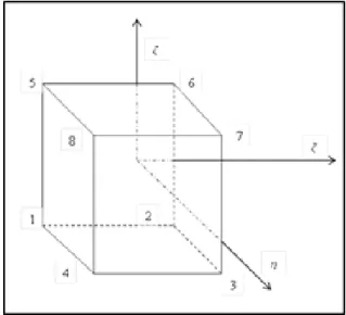
2.5 The eight-node hexahedron element ...69
2.6 The four-node tetra element ...73
2.7 The six-node prism element ...76
2.8 The five-node pyramid element ...79
CHAPTER 3 OBJECT-ORIENTED PROGRAMMING ...83
3.1 Object-Oriented programming ...83
3.2 Object-oriented programming in calculating elemental matrix and residual ...84
3.3 Comparison with the flow-based programming ...100
4.1 Introduction ...101
4.2 NACA0012 ...101
4.2.1 Case 1 (Re=2.88 10× 6, M=0.15, = 0, 10 and 15, hybrid mesh) .... 101
4.2.2 Case 2 (Re=2.88 10× 6, M=0.15, = 0, 10 and 15, tetra mesh) ... 112
4.2.3 Comparison between the tetra mesh and hybrid mesh... 123
4.3 DLR F11 model ...128
CONCLUSION ...139
APPENDIX I Data pre-processing interface ...141
Table 2.1 Numerical Integration ...68
Table 2.2 Coordinates ...69
Table 2.3 Shape Functions ...70
Table 2.4 Numerical Integration ...72
Table 2.5 Coordinates ...73
Table 2.6 Shape Functions ...74
Table 2.7 Numerical Integration ...75
Table 2.8 Coordinates ...76
Table 2.9 Shape Functions ...77
Table 2.10 Numerical Integration ...78
Table 2.11 Numerical Integration ...78
Table 2.12 Coordinates ...80
Table 2.13 Shape Functions ...80
Table 2.14 Five-Point Numerical Integration ...82
Table 2.15 Six-Point Numerical Integration ...82
Table 4.1 Lift coefficient for 10 ...128
Table 4.2 Lift coefficient for 15 ...128
Figure 2.1 Eight-node hexahedron element ...69
Figure 2.2 Four-node tetra element ...73
Figure 2.3 Six-node prism element ...76
Figure 2.4 Five-node pyramid element ...79
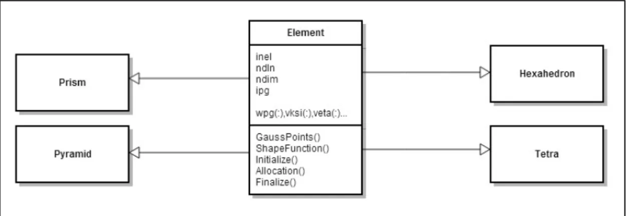
Figure 3.1 The class Element and its four derived types ...84
Figure 3.2 Class Element ...85
Figure 3.3 Class Tetra ...86
Figure 3.4 Element initialization ...87
Figure 3.5 Shape function and integration points ...87
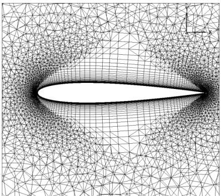
Figure 4.1 Mesh around the airfoil (hybrid mesh) ...102
Figure 4.2 Density (M=0.15, Re=2.88 10× 6, α = 0°) ...103
Figure 4.3 (M=0.15, Re=2.88 10× 6, α = 0°) ...104
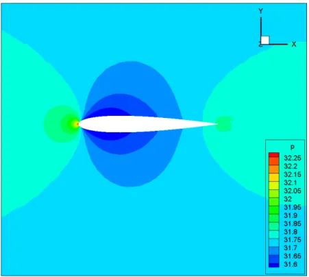
Figure 4.4 Pressure (M=0.15, Re=2.88 10× 6 , α = 0°) ...104
Figure 4.5 Velocity (M=0.15, Re=2.88 10× 6, α = 0°) ...105
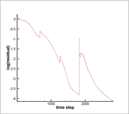
Figure 4.6 Evolution of residual with time ...105
Figure 4.7 Evolution of ε with time ...106
Figure 4.8 Density (M=0.15, Re= 6 2.88 10× , α = 10°) ...106
Figure 4.9 (M=0.15, Re=2.88 10× 6 , α = 10°) ...107
Figure 4.10 Pressure (M=0.15, Re=2.88 10× 6, α = 10°) ...107
Figure 4.12 Evolution of residual with time ...108
Figure 4.13 Evolution of ε with time ...109
Figure 4.14 Density (M=0.15, Re=2.88 10× 6, α = 15°) ...109
Figure 4.15 (M=0.15, Re=2.88 10× 6, α = 15°) ...110
Figure 4.16 Pressure (M=0.15, Re=2.88 10× 6 , α = 15°) ...110
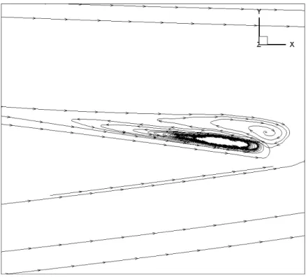
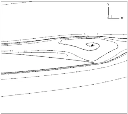
Figure 4.17 Velocity (M=0.15, Re=2.88 10× 6 , α = 15°) ...111
Figure 4.18 Evolution of residual with time ...111
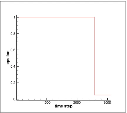
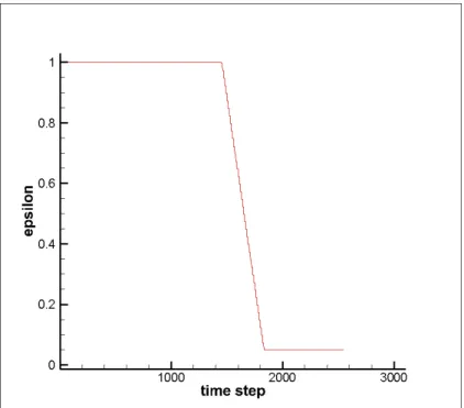
Figure 4.19 Evolution of ε with time ...112
Figure 4.20 Mesh around the airfoil (tetra mesh) ...113
Figure 4.21 Density (M=0.15, Re=2.88 10× 6 , α = 0°) ...114
Figure 4.22 (M=0.15, Re=2.88 10× 6, α = 0°) ...114
Figure 4.23 Pressure (M=0.15, Re=2.88 10× 6, α = 0°) ...115
Figure 4.24 Velocity (M=0.15, Re=2.88 10× 6, α = 0°) ...115
Figure 4.25 Evolution of residual with time ...116
Figure 4.26 Evolution of ε with time ...116
Figure 4.27 Density (M=0.15, Re=2.88 10× 6, α = 10°) ...117
Figure 4.28 Pressure (M=0.15, Re=2.88 10× 6 , α = 10°) ...117
Figure 4.29 (M=0.15, Re= 6 2.88 10× , α = 10°) ...118
Figure 4.30 Velocity (M=0.15, Re=2.88 10× 6, α = 10°) ...118
Figure 4.31 Evolution of residual with time ...119
Figure 4.32 Evolution of ε with time ...119
Figure 4.33 Density (M=0.15, Re= 6 2.88 10× , α = 15°) ...120
Figure 4.35 (M=0.15, Re=2.88 10× 6, α = 15°) ...121
Figure 4.36 Velocity (M=0.15, Re=2.88 10× 6 , α = 15°) ...121
Figure 4.37 Evolution of residual with time ...122
Figure 4.38 Evolution of ε with time ...122
Figure 4.39 Cp (M=0.15, Re=2.88 10× 6 , α = 0°) ...123
Figure 4.40 Cp around the trailing edge ...124
Figure 4.41 Cp (M=0.15, Re=2.88 10× 6, α = 10°) ...124
Figure 4.42 Cp around the leading edge ...125
Figure 4.43 Cp around the trailing edge ...125
Figure 4.44 Cp (M=0.15, Re=2.88 10× 6, α = 15°) ...126
Figure 4.45 Cp around the leading edge ...126
Figure 4.46 Cp around the trailing edge ...127
Figure 4.47 Mesh of the whole domain ...129
Figure 4.48 Mesh around the fuselage ...129
Figure 4.49 Mesh around the wing ...130
Figure 4.50 Pressure at z=30 in ...131
Figure 4.51 χ at z=30 in ...131
Figure 4.52 Cp contour of slat at 17% of span ...132
Figure 4.53 Cp contour of slat at 50% of span ...133
Figure 4.54 Cp contour of slat at 70% of span ...133
Figure 4.55 Cp contour of slat at 95% of span ...134
Figure 4.56 Cp contour of main-wing at 17% of span ...134
Figure 4.57 Cp contour of main-wing at 50% of span ...135
Figure 4.59 Cp contour of main-wing at 95% of span ...136
Figure 4.60 Cp contour of flap at 17% of span ...136
Figure 4.61 Cp contour of flap at 50% of span ...137
Figure 4.62 Cp contour of flap at 70% of span ...137
c Speed of sound
p
C Specific heat capacity
v
C Volumetric heat capacity
d Wall distance
D Strain tensor
e Total energy
E Total energy per unit volume
v
f Body force vector
adv
F Advection flux
diff
F Diffusion flux
s
F Heat source flux
he Characteristic length of an element
i Internal energy
I Identity matrix
J Jacobian matrix of geometric transformation
k Thermal conductivity
[ ]
K Global stiffness matrix[ ]
M Global mass matrixn Unit normal outward pointing vector
[ ]
N Block diagonal matrix of shape functionsi N Shape function p Pressure Pe Peclet number r Heat source R Residual vector Re Reynolds number t Time T Temperature
V Vector of conservative variables
{ }
Vh Vector of nodal unknownsW Test function
, ,
x y z Cartesian coordinates , ,
ξ η ζ Coordinates of the reference domain
Ω Domain of integration Γ Boundary of the domain
σ Stress tensor ρ Density ν Dynamic viscosity t ν Turbulent viscosity τ Stabilization matrix c
ς Sensor of pressure variation p v C C γ = Adiabatic index
ω Module of flow vorticity
1, 2 , , 2, 3, 1, 2, b b w w v v c c σ c c c c k Empirical constants 1, 2, 3, , , v v v w f f f f g r Intermediate functions
Generalities
Fluid dynamics is the branch of mechanics that studies the mechanics and heat transfer related to the motion of fluids, including liquids and gases. Common examples of phenomena involving fluid dynamics include airflow around an aircraft, ocean currents, engine turbines, and the circulatory system of the human body. Fluid dynamics has two subdisciplines. One is hydrodynamics, which deals with liquids in motion. The other is aerodynamics, which deals with air and gases in motion, especially flows over a plane.
The development of fluid dynamics can be traced back to Archimedes, who provided the fundamental principles of hydrostatics in his work On Floating Bodies (Archimedes, 287BC-212BC). He was the first person who summarized the mechanics of static fluid. Newton contributed significantly to fluid dynamics in his work The Mathematical Principles of Natural Philosophy, in which he discussed fluid resistance and wave motion. He established fluid dynamics as an independent branch of mechanics. The French engineer Navier (Navier, 1823) and the British mathematician Stokes (Stokes, 1845) independently proposed a theory showing how viscosity can have an effect on a fluid. This theory has led to the development of the Navier-Stokes equations.
Mathematically, it is difficult to find the exact solution for the Navier-Stokes equations. Computational fluid dynamics (CFD) methods have become powerful tools for solving such equations as a supplement to experimental analysis of complex fluid phenomena. CFD includes the finite element method (FEM), the finite volume method (FVM), the finite difference method, etc. FEM is commonly used in such industries as aerospace, mechanical manufacturing, nuclear power, and civil engineering. The first idea of FEM can be traced back to ancient times when mathematicians calculated the circular constant using polygons to approximate a circle. With the development of high-speed computation and new algorithms, FEM has gained in popularity over the years. There are currently numerous commercial FEM
software products on the market, such as Nastra (MSC Software 2015), Ansys (Ansys, 2015), and Abaqus (Dassault Systèmes, 2015).
When a fluid moves smoothly and steadily in parallel layers, the flow is said to be laminar. When a fluid moves in irregular paths, the flow is said to be turbulent. In compressible turbulent flows, the velocity, pressure, density, viscosity, and temperature fluctuate. A small Reynolds number usually results in laminar flow, and a high Reynolds number usually results in turbulent flow. The flow is said to be transitional when the Reynolds number is high but not sufficiently high to make the flow turbulent.
Turbulence will start to appear as the Reynolds number increases. Turbulence is a random phenomenon, and it is hard to predict the variations in both space and time. It is usually treated statistically. The velocity field is three-dimensional (3D) and rotational. Turbulence has a diffusive character; it increases the rate of homogenization, the transport of mass, momentum, and energy. It also has a dissipation characteristic; kinetic energy is rapidly converted into internal energy.
The earliest description of turbulence can be traced back to Leonardo da Vinci (Lumley, 1997). In 1877, Boussinesq (Boussinesq, 1877) proposed the hypothesis that turbulent stresses are linearly proportional to mean strain rates. This hypothesis greatly influenced the development of the study of turbulence. In 1883, Osborne Reynolds (Reynolds, 1883) conducted experiments to visualize the turbulence phenomenon in circular conduits. He introduced the idea of decomposing the flow variables into mean and fluctuating parts. This led to the development of the Reynolds-averaged Navier-Stokes (RANS) equations. Wilcox developed more complicated Favre-averaged Navier-Stokes equations (Wilcox, 1994). Using Reynolds averaging, we can derive a simple form of the averaged Navier-Stokes equations. The equation for conservation of mass stays the same. The equation for conservation of momentum has an additional Reynolds stress term: −ρui′⊗u′j . The equation for conservation of energy has an additional turbulence flux term.
Because many engineering problems are turbulent, turbulence modeling is crucial in CFD. The RANS model has both linear and nonlinear eddy viscosity models. The linear eddy viscosity models can be categorized based on the number of equations.
The first type of models is the zero-equation model. Zero-equation models do not introduce any new equations and simply use the existing variables. They define a relationship between the turbulent flux and the averaged value of variables. Prandtl proposed a mixing-length model. Van Driest (Van Driest, 1956) developed a viscous damping correction for the length model. The Cebeci-Smith model (Smith and Cebeci, 1967) refined the mixing-length concept. The Baldwin-Lomax model (Baldwin and Lomax, 1978) proposed a model that is suitable for high-speed flows with thin boundary layers. Another example is the Johnson-King model, which is suitable for turbulent boundary layer flows with strong adverse pressure gradients.
The second type of models is the one-equation model. One-equation models introduce one turbulent transported variable. We cite four models: Prandtl’s one-equation model, the Spalart-Allmaras model (Spalart and Allmaras, 1992), the Baldwin-Barth model (Baldwin and Barth, 1990), and the Rahman-Siikonen-Agarwal Model (Rahman et al, 2011).
The third type of models is the two-equation model. Two-equation models introduce two turbulent transport equations. Two-equation models are among the most commonly used turbulence models. Most of the models introduce the turbulent kinetic energy. Here we cite the RNG k−ε model (Yakhot et al, 1992), Wilcox’s k−ω model (Wilcox, 1988), the SST
k−ω model (Menter, 1994), and the Launder-Sharma model (Launder and Sharma, 1974).
Literature review
Many authors have proposed numerical methods to solve compressible RANS equations. Some numerical methods are FEMs. Our research is mainly based on the following works. El Kadri (El kadri, 1995) presented in his thesis presented a finite element model for two
dimensional flows. Soulaïmani and Ben Haj Ali (Soulaïmani and Ben Haj Ali, 2003) proposed a parallel-distributed computing-based approach for the solution of some multiphysics problems. They validated the method on the Agard 445.3 airfoil. Soulaïmani et al (Soulaïmani et al, 2004) proposed an efficient parallel-distributed methodology for solving multiphysics problems. They validated the results on Agard 445.6 airfoil. Ben Haj Ali and Soulaïmani (Ben Haj Ali and Soulaïmani, 2010) proposed a stabilized FEM for solving the compressible Navier-Stokes equations combined with the Spalart-Allmaras model. They validated the code on the 3D boundary layer over a flat plate and on the ONERA-M6 wing. Rebaine (Rebaine, 1997) proposed a numerical method for two-dimensional (2D) compressible laminar and turbulent flows. Rebaine and Soulaïmani (Rebaine and Soulaïmani, 2001) proposed an FEM for simulation of 2D internal compressible turbulent flows. They validated the method in 2D supersonic and thrust augmenting ejectors. Soulaïmani et al (Soulaïmani et al, 2002b) proposed a conservative finite element formulation for the coupled fluid/mesh interaction problem. Soulaïmani et al (Soulaïmani et al, 1994) proposed an FEM for simulation of 2D internal compressible turbulent flows. Soulaïmani and Fortin (Soulaïmani and Fortin, 1994) proposed a method to solve the Navier-Stokes and Euler equations in a conservative form by using the conservation variables.
Aside from FEM, some numerical methods involving FVM (Finite Volume Method) are also proposed for solving the Navier-Stokes equations. Caughey and Jameson (Caughey and Jameson, 2003) proposed an FVM for transonic flow calculation. They used this method on swept wings and wing-cylinder combinations. They showed that the FVM has the advantage of adaptability to treat a variety of complex configurations. Hafez (Hafez, 1995) proposed a cell-vertex finite volume formulation using local finite element approximations to solve inviscid and viscous compressible flow equations on unstructured grids. Feistauer et al (Feistauer et al, 1995) proposed a numerical modeling of inviscid as well as viscous gas flow. The method is based on an upwind flux vector splitting finite volume scheme on various types of unstructured grids.
Many authors have also proposed various techniques to solve the RANS equations. Pontaza and Reddy (Pontaza and Reddy, 2003) proposed a formulation of a spectral/hp algorithm to the numerical solution of the Navier-Stokes equations governing stationary incompressible and low-speed compressible flows. Rachowicz (Rachowicz, 2000) presented a technique of approximating boundary layers in viscous flow simulations with significantly stretched elements for compressible Navier-Stokes equations. Klaij et al (Klaij et al, 2006) presented a space-time discontinuous Galerkin element method for the compressible Navier-Stokes equations. They showed the space-time setting, derived the weak formulation, and discussed the choices for the numerical fluxes. Nazarov and Hoffman (Nazarov and Hoffman, 2010) presented an adaptive FEM for the compressible Euler equations. They used continuous piecewise linear approximation in space and time with componentwise weighted least-squares stabilization of convection terms and residual-based shock-capturing. Kellogg and Liu (Kellogg and Liu, 2000) developed a finite element formulation for the 2D nonlinear time-dependent compressible Navier-Stokes equations on a bounded domain. Cao (Cao, 2005) presented methods for improving the adaptive finite element simulation of compressible Navier-Stokes flow via a posteriori error estimate analysis. He used the moving space-time FEM to globally discretize the time-dependent Navier-Stokes equations on a series of adapted meshes. Banas (Banas, 2002) presented an implementation of the Newton-Krylov-Schwarz methodology for stabilized adaptive finite element approximations of compressible Navier-Stokes equations. Baruzzi et al (Baruzzi et al, 1995) presented numerical solutions for transonic inviscid and viscous laminar flows using higher-order dissipation. Martinez and Gartling (Martinez and Gartling, 2004) presented the derivation and justification for various low-speed approximations of the fully compressible Navier-Stokes equations. He and Li (He and Li, 2010) presented a fully discrete penalty FEM for the 2D time-dependent Navier-Stokes equations. Kweon (Kweon, 2000) presented a linearized steady-state compressible viscous Navier-Stokes system with an inflow boundary condition. Shan and Hou (Shan and Hou, 2009) proposed a fully discrete stabilized FEM based on two local Gauss integrations for the 2D time-dependent Navier-Stokes equations. Compared with other stabilized methods, this approach does not require specification of a stabilization parameter or calculation of higher-order derivatives. Burman (Burman, 2000) proposed
adaptive streamline diffusion FEMs with error control for compressible flow in one, two, and three dimensions. Karagiozis et al (Karagiozis et al, 2009) proposed a numerical method to solve the compressible Navier-Stokes equations around objects of arbitrary shape using Cartesian grids. This method is suitable for compressible flows without shocks. Lomtev and Karniadakis (Lomtev and Karniadakis, 1999) presented the foundations of a new discontinuous Galerkin method for simulating compressible viscous flows with shocks on standard unstructured grids. This method is based on a discontinuous Galerkin formulation for both advective and diffusive contributions. Kirk and Carey (Kirk and Carey, 2008) applied the streamline upwind/Petrov-Galerkin (SUPG) method to the unsteady compressible Navier-Stokes equations in conservation-variable form. They used a modified approach for interpolating the inviscid flux terms in the SUPG finite element formulation for the spatial discretization. They used second-order accurate time discretization. Li et al (Li et al, 1998) developed finite element-based methodology for the numerical simulation of the compressible Navier-Stokes equations on unstructured triangular meshes. They used a Galerkin finite-element discretization in space and an explicit Runge-Kutta multistage integration in time. Nigro et al (Nigro et al, 1998) presented the implementation of a local physics preconditioning mass matrix for a unified approach of 3D compressible and incompressible Navier-Stokes equations using an SUPG finite element formulation and GMRES implicit solver. Erwin et al (Erwin et al, 2013) developed a high-order flow solver for compressible flows using a stabilized finite element approach. They used streamline/upwind Petrov-Galerkin discretization for the Navier-Stokes equations, and they used a fully implicit methodology for advancing the solution at each time step.
To test our code, there are many test cases that we can use as comparisons. Liu and Li (Liu and Li, 2001) developed an unstructured algorithm for the computation of compressible RANS equations. The turbulence models they chose were the Baldwin-Lomax model and the Baldwin-Barth model. They validated the results on a flat plate, an RAE2822 airfoil, and an NACA0012 airfoil. Kersken et al (Kersken et al, 2012) proposed a computational method for solving the compressible RANS equations. They validated the method on the benchmark problem Stardard Configuration 10 and a modern ultra-high bypass ration fan. Bassi and
Rebay (Bassi and Rebay, 2014) proposed a high-order accurate discontinuous FEM for the numerical solution of the compressible Navier-Stokes equations. They showed that the method is robust in all test cases.
The Spalart-Allmaras model uses only one equation to model turbulent viscosity. The equation has one nonlinear diffusion term, one destruction term, and one production term. The Boussinesq hypothesis is employed in the model; the Reynolds stress is linearly proportional to the mean stain rates. It has advantages for applications involving wall-bounded flows and boundary layers subjected to adverse pressure gradients.
Numerous research studies have demonstrated that the Spalart-Allmaras model performs well on the external flow. Yan et al (Yan et al, 2011) validated the Spalart-Allmaras model for turbulent flow past a square cylinder. They obtained results that reasonably agree with the existing experimental results and discovered that the fluctuating pressure is more sensitive to the change in the afterbody shape. Paciorri et al (Paciorri et al, 1998) validated the Spalart-Allmaras turbulent model for hypersonic flows. They discovered that for flows involving laminar separation and turbulent reattachment, the model obtained results which agreed with the experimental data. They also demonstrated that the model correctly predicted the turbulent separation. Geng et al (Geng et al, 2011) validated four turbulence models, one of which was the Spalart-Allmaras model, on 2D supersonic expansion-compression and hypersonic flows. They obtained results that matched the experimental data and recommended compressibility for hypersonic flows at a high angle of attack. Roy and Blottner (Roy and Blottner, 2003) validated the model on hypersonic transitional flows. They presented the documentation procedure, numerical accuracy, model sensitivity, and model validation. Coratekin et al (Coratekin et al, 2004) evaluated four upwind schemes and four turbulence models, one of which was the Spalart-Allmaras model, in hypersonic flows. Their results showed that the k−ω model provided the best prediction in cases of separation. Kong et al (Kong et al, 2012) conducted simulations of crossing shock wave/turbulent boundary layer interaction using three turbulence models: Wilcox’s k−ωmodel, the Spalart-Turbulence model, and the SST model. Their results showed that the SST model achieved
better results in the pressure and velocity vector, and all three models over-predicted the heat transfer coefficient. Nordanger et al (Nordanger et al, 2015) tested three solvers on a fixed NACA0012 airfoil at a high Reynolds number, one of which used the coupled Navier-Stokes equations with the Spalart-Allmaras turbulence model. They used the three solvers for flows over a NACA0012 airfoil at Reynolds number 6
3 10× at four different angles of attack. They noticed that beyond the angle of attack of 15°, it is difficult to predict lift and drag when the
flow enters the stall regime. They also noticed that increasing the element order from 1 to 2 will give better approximation of lift, drag, and pressure coefficients for the Spalart-Allmaras model.
Several research studies have simulated the turbulent flows using averaged Navier-Stokes equations and the Spalart-Allmaras model. Soulaïmani (Soulaïmani, 2001) presented a stabilized finite element formulation for solving compressible flows. He presented three stabilization techniques: the SUPG formulation, the DG method, and the EBS method. Wervaecke et al (Wervaecke et al, 2012) presented a RANS-based Spalart-Allmaras SUPG formulation for 2D and 3D turbulent compressible flows. They tested this model on NACA0012 airfoil, RAE2822 airfoil, S809 airfoil, 3D ONERA M6 wing, and 3D turbulent flat plate.
Some authors have proposed methods to modify the Spalart-Allmaras model to achieve better performance in different cases. Liu et al (Liu et al, 2011) modified the Spalart-Allmaras model with relative helicity density to improve the predictive accuracy for corner separation flow. Yan et al (Yan et al, 2014) conducted a simulation of S825 airfoil using the Spalart-Allmaras model and compared the results to experimental data. They proposed using different values of parameter C for the non-separating region and the separating region. b1 Aupoix and Spalart (Aupoix and Spalart, 2003) introduced two extensions to the Spalart-Allmaras model to account for wall roughness. Developed independently by Boeing and ONERA, the two extensions assume a non-zero-eddy viscosity at the wall and change the definition of the distance d. Rung et al (Rung et al, 2003) proposed changing constant C to b1 a function of the strain rate for nonequilibrium flows. Deck et al (Deck et al, 2002) presented
an extension of the Spalart-Allmaras model to compressible supersonic flows. This model achieved good results for simulations on a missile. De Santis (De Santis, 2014) developed a high-order residual distribution scheme for compressible RANS equations. He changed the definition of the working variable to deactivate the production and destruction terms of the turbulence model equations when turbulent viscosity is negative. He also eliminated the diffusion contribution in the source term when the turbulent viscosity is negative. He tested the model in several 2D and 3D cases. Ishiko et al (Ishiko et al, 2014) proposed an extended nonlinear algebraic constitutive relation for the Reynolds stress tensor and modifications to improve predictions for the free jet-based Spalart-Allmaras model. Khurram et al (Khurram et al, 2012) presented a multiscale FEM with the Spalart-Allmaras turbulence model for 3D detached-eddy simulation. They decomposed the scalar field into coarse scales and fine scales. They showed that this method provided effective stabilization in turbulent computations where reaction-dominated effects strongly influence the boundary layer prediction. Lorin et al (Lorin et al, 2007) proposed a stable numerical method preserving the positivity of the turbulent viscosity in the Spalart-Allmaras model. They validated the method on the 3D boundary layer over a flat plate.
As with most numerical methods, an appropriate stabilization is important for obtaining optimal performance. Soulaïmani and Fortin (Soulaïmani and Fortin, 1994) proposed a definition of the stabilization matrix τ for several dimensions. They also proposed an artificial viscosity for shock capturing. Tezduyar and Senga (Tezduyar and Senga, 2006) proposed a definition of the SUPG stabilization matrix τ and a shock-capturing operator. Wong et al (2000) presented a stabilized finite element algorithm and proposed a definition of a stabilization matrix τ . They showed that this new matrix represents a dramatic improvement over more standard choices. Wang et al (Wang et al, 2014) presented high-order discontinuous Galerkin and SUPG methods for solutions of 3D viscous flows and 2D turbulent flows. They also proposed a definition of the matrix τ .
Objective of thesis
The objective of this thesis is to modify an existing in-house code (Ben Haj Ali and Soulaïmani, 2010) to enhance its capability to solve 3D compressible turbulent flows. The original code is limited to one type of element, and we expand its capacity to allow the use of several types of elements in a hybrid mesh.
We then must validate our code. We used our code to simulate the turbulent flows over a 3D wing model and a fuselage. The wing model we chose for the validation was extruded from NACA0012. The fuselage we chose was the DLR F11 model. Currently there are many references available for these two cases, and we compared our results with other numerical and experimental results.
Plan of thesis
Chapter 1 introduces the governing equations and the use of FEM. The Navier-Stokes equations are presented: the equations describing conservation of mass, conservation of momentum, and conservation of energy. The weak form of the Navier-Stokes equations is then developed. We show how we formulated the spatial and time discretizations, computed the elemental matrix and elemental residual for each type of element, and applied the initial and boundary conditions. This chapter also shows the stabilization and shock-capturing techniques. Finally, we use the Newton-Raphson method and the GMRES algorithm to solve the system of equations.
Chapter 2 describes the four elements used and the numerical integration. The four elements are hexahedrons, tetras, prisms, and pyramids. This chapter also shows how we obtained the shape functions and integration points for each type of element.
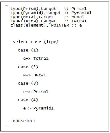
To facilitate the programming of the elemental matrix and residual for different types of elements, we used object-oriented programming in Fortran 2003. Chapter 3 presents the use
of the object-oriented programming method and shows how we realized this concept in our code. We then make a comparison with the non-object-oriented programming.
Chapter 4 discusses the results we obtained after running our code on several test cases. We also make a comparison with other numerical and experimental results.
GOVERNING EQUATIONS
1.1 Introduction
Our goal is to establish a finite element model to simulate external compressible flows. The internal properties of the flow are already known: the dynamic viscosityμ, the thermal conductivity k , and the heat capacities C and p C . We describe the state of the flow using v
the density ρ , the velocity vector U, the pressure p , and the temperature T . These unknown variables are then solved using the Navier-Stokes equations, which describe the conservation of mass, momentum, and energy.
The mass conservation law is expressed in the continuity equation. For any flow of mass m,
( ) 0
d m dt =
(1.1)
The momentum conservation law is expressed by Newton’s second law:
( )
d m
dt u =
F(1.2)
The left side denotes the time rate of momentum per unit mass. The right side denotes the sum of applied forces, including body forces and surface forces.
The idea of energy conservation is expressed in the equation describing conservation of energy, which shows that the time rate of change for the total energy of a control volume equals the sum of the rate of work performed by the surface force, the body force, the rate of heat transfer, and the rate of heat source in the volume:
s v
dE
r dt = ⋅ + ⋅ − ∇ ⋅ +f U f U q
(1.3)
Another necessary equation is the equation of state. For gas, the temperature, density and pressure are not independent quantities but are connected: F p( , , ) 0ρ T = . For Mach numbers smaller than 5, we can use the perfect gas law.
To solve this system of partial differential equations, we also add the proper initial conditions and boundary conditions. This system of equations can model laminar and turbulent as well as compressible and incompressible flows. This system of equations is too complex to solve analytically and usually requires the use of numerical methods. To solve this system of equations numerically, we must choose the proper dependent variables and write the system of equations in a proper form to facilitate programming. The Navier-Stokes equations can be written in several forms. In the following sections, we will present in detail the form we used and how to implement the finite element method.
1.2 Conservative form in conservative variables
There are three general forms that we can use: the conservative form, the nonconservative form, and the conservative form with conservative variables. We write each of the Navier-Stokes equations in its conservative form with conservative variables (El Kadri, 1995).
Let ρ be the density and u be the vector of velocities, then we define the momentum of unit mass:
ρ
=
U u (1.4)
Let e be the total energy and i be the internal energy, then we define the total energy of the unit mass:
E=ρe (1.5)
where 1 2
2
e i= + u .
We can now write the system of equations in its conservative form with conservative variables.
The continuity equation reads
( ) 0 t ρ ∂ +∇⋅ = ∂ U (1.6)
The momentum equations are
( ) p v t ρ ρ ∂ +∇⋅ ⊗ +∇ −∇⋅ = ∂ U U U σ f (1.7)
The energy equation is
( ) ( ) v E E p r t ρ ρ ∂ +∇⋅ + = ∇ ⋅ ⋅ − ∇ ⋅ + ⋅ + ∂ U U q f U σ (1.8)
The stress tensor is defined as
( )u = ∇⋅ +λ( u) 2μD
σ (1.9)
where the tensor D has components
, , 1 ( ) ( ) 2 ij ij i j j i D =D u = u +u (1.10)
μ and λ are Lamé constants, and they can be connected by Stokes’s law:
2μ+3λ=0 (1.11)
For air, the heat transfer can be obtained by Fourier’s law:
k T
= − ∇
q (1.12)
Along with the ideal gas law, the equations can be solved.
1.3 Dimensionless form
To obtain better insight into the problem, we apply nondimensionalization to the system of equations. The geometry stays the same but is scaled. In addition, the scaled system has the same physical characteristics as the original one. In this way, we can find the solution for problems with the same boundary conditions but with different scales in the geometry.
We convert variables to their dimensionless form using scales denoted by index r:
* * * 2 * * * 2 * * 2 r r r r r r r r r r v p p i t i t L T x T x L C ρ ρ ρ ρ μ μ μ = = = = = = = = u u u u u u u (1.13)
To simplify the notation, we omit the star. The unit momentum, stress tensor, heat flux, total energy per unit mass, and pressure are defined respectively as:
ρ = U u (1.14)
(
)
1 2 1 ( ) ( ) Re 3 Re T = ∇ + ∇ − ∇⋅ u u u u I σ (1.15) Re Pr T γ = − ∇ q (1.16) 2 ( ) 2 E=ρe=ρ T+ u (1.17) ( 1) p= −γ ρT (1.18)When we substitute equation (1.14) into equation (1.15), we can write the stress tensor:
( ) ( )
( )
2 1 1 2 ( ) ( ) ( ) Re 3 T T T ρ ρ ρ ρ ρ = − ⋅ ∇ + ∇ ⋅ − ⋅ ∇ u u U U U I σ σ (1.19)When we substitute equations (1.14) and (1.17) into equation (1.16), we can write the heat flux as 2 2 ( ) Re Pr 2 E γ ρ ρ = − ∇ − U q (1.20)
When we substitute equations (1.14) and (1.17) into equation (1.18), we can write the pressure as 2 ( 1) 2 p γ E ρ = − − U (1.21)
The dimensionless form of the set of conservation equations is ( ) 0 t ρ ∂ +∇⋅ = ∂ U (1.22) ( ) p v t ∂ +∇⋅ ⊗ +∇ −∇⋅ = ∂ U U u σ f (1.23)
[
( )]
( . ) v E E p t ∂ +∇⋅ + = ∇ ⋅ − ∇ ⋅ + ⋅ ∂ u σu q f U (1.24)The dimensionless form is identical to the original one, but in the second system we introduce two similarity parameters: Reynolds number Re r r r
r
L ρ
μ
= u and Prandtl number
Pr r r r Cp k μ = .
The Reynolds number is the ratio of inertial forces to viscous forces. A small Reynolds number indicates that the flow is dominated by diffusion. Alternatively, a large Reynolds number means that the flow is dominated by convection.
The Prandtl number is the ratio of kinematic viscosity to thermal diffusivity. ≪ 1 indicates that the flow has dominantly thermal diffusivity. ≫ 1 indicates that the flow has dominantly kinematic viscosity. The variation of the Prandtl number is relatively small, and we use Pr=0.72.
We can also define another similarity parameter, which is the product of Re and Pr, known as the Peclet number:
P Re Pr r r r r r r r r r Cp e k v ρ μ μ = = u L =u L (1.25)
v is the thermal diffusivity. The Peclet number is the ratio of the rate of advective transport of heat by the flow to the diffusive rate of heat. A large Pe means that the energy of the flow is dominated by the advective transport of heat.
1.4 Vectorial form
The system of equations can be written in vectors:
, , ,
adv diff S
t + i i = i i +
V F F F (1.26)
V represents the vector of conservative variables:
E ρ = V U (1.27) adv i
F is the advection flux:
( ) i adv i i ij i p E p δ ρ ρ = + + U U F U U (1.28) diff i
(
)
(
)
1 2 3 1 2 3 , 0 , , , , T diff i i i i T i i i kTi σ σ σ σ σ σ = ⋅ − F u (1.29) sF is the source term:
0 s v v ρ = ⋅ F f f U (1.30) 1.5 Weak formulation
In order to use FEM to solve this system of equations, we must write it in the weak form. We first multiply the equations with a test function W and integrate:
, , , .( adv diff S) t i i i i d Ω + − − Ω=
W V F F F 0 (1.31)The weighted residuals are realized by the Galerkin method. We use the Gauss theorem on the diffusion term and convert the strong form of the system of equations to its weak form:
, , ,
( )
e e
adv S diff diff
t i i i i i i
e e
d d d
Ω + − Ω+ Ω Ω − Γ Γ=
W V F F
W F
WF n 0 (1.32)The domain Ω is divided to subdomains Ω , and n is the unit outward-pointing normal e
vector to Γ . The surface integration in the weak allows us to easily apply the boundary conditions.
1.6 Spatial discretization
The domain is meshed using four kinds of elements: 4-node tetras, 8-node hexahedrons, 6-node prisms, and 5-node pyramids.
The integration of any function f over the domain Ω can be written as
( , , ) ( , , ) e e e f x y z d f x y z d Ω Ω Ω =
Ω
(1.33)The conservative variables V are approximated by the products of the shape functions and coefficients, which are evaluated at the nodes (Dhatt and Touzot, 1981):
1 2 1 2 1 ( ) ( ) . ( ) ( ) , ,... . . ( ) n k k n k n i i i N i N N N i = = =
V V V V V (1.34)where V(1)=ρ, (2)V =ρu, (3)V =ρv, (4)V =ρw, (5)V =ρe. The number n of shape functions per element is also the number of nodes per element. By the Galerkin method, we also use the same shape functions for the test functions.
The elements forming the mesh are not identical in shape or size. It is more convenient to transform the domain Ω to the reference domain e Ω (Dhatt and Touzot, 1981). The r
reference coordinates are denoted by ( , , )ξ ξ η ζi . The derivative of the function ( , , )f x y z with respect to ξi is
1 2 3 1 2 3 . ( , , ) , ,... . . i i i i f f N N N f x y z f ξ ξ ξ ξ ∂ ∂ ∂ ∂ = ∂ ∂ ∂ ∂ (1.35)
The integration of the function f x y z( , , ) over the domain Ωe can now be written as
( , , ) ( , , ) det( ) e r e r f x y z d f ξ η ζ d Ω Ω Ω = Ω
J (1.36)where J is theJacobian matrix of the transformation:
x y z x y z x y z ξ ξ ξ η η η ζ ζ ζ ∂ ∂ ∂ ∂ ∂ ∂ ∂ ∂ ∂ = ∂ ∂ ∂ ∂ ∂ ∂ ∂ ∂ ∂ J (1.37) 1.7 Time discretization
To discretize the time-derivative term, we use the first-order forward finite difference method: ( ) ( ) ( ) ( ) t t t t t t t ∂ = + Δ − + Ο Δ ∂ Δ V V V (1.38)
t
Δ can be calculated using
( ) e e h t CFL c Δ = + u , where e
h is the minimum length between the nodes of an element and c is the speed of sound.
1.8 SUPG stabilization
The use of the weak form by the Galerkin method will produce some numerical instability, especially if the convection flux is dominant. The stabilization method used here is SUPG. This method is popular in solving transport equations. It introduces a supplementary term to the standard Galerkin method and reinforces the stability inside the element (Soulaïmani and Fortin, 1994). This additional term adds artificial diffusion in the flow direction:
(
)
, , , ( ) e i i t ij j i e i s i d x Ω ∂ + − − Ω ∂
A W Vτ A V K V F (1.39)The τ matrix has the dimension of time and depends on the element geometry. There are various definitions of this matrix. We need to choose a τ matrix without introducing excessive diffusion to the solution on the boundary layer and across the shock wave. Soulaïmani and Fortin (Soulaïmani and Fortin, 1994) proposed a τ matrix:
1 ( ) ij j h i c R τ ς − =
A (1.40) where i ij j c x ζ ∂ =∂ is the transformation matrix from the actual element to the reference
element. ( )ς Rh is defined as ( ) min ,1 3 h h R R ς = (1.41)
where 2 h h R μ
= u is the local Reynolds number, μ is the dynamic viscosity, and h is the characteristic length of the element.
This method will produce an artificial viscosity with order
2
h
u
, so there will be a large numerical diffusion, especially in the boundary layer. Ben Haj Ali and Soulaïmani (Ben Haj Ali, 2008; Ben Haj Ali and Soulaïmani 2010) proposed a new definition of the τ matrix to accommodate stretched elements. This diagonal matrix is defined as
2
h τ
λ
= I (1.42)
where I is the identity matrix and λ is the largest eigenvalue of the advection matrix: c
λ= u + . h is a characteristic length of the element defined as h=min xi−xj , where i
and j are the nodes of the element.
1.9 Shock capturing
Along with the stabilization term, we add another term to capture the oscillations caused by the large gradients. This additional numeric dissipation across the shock waves will further add numerical stability:
[ ]
e c e d μ Ω ∇ ∇ Ω
W V (1.43)There are various definitions of the shock capturing matrix. Soulaïmani and Fortin (Soulaïmani and Fortin, 1994) proposed the following definition of the shock capturing operator:
(
)
min , 2 k c C h μ = τR(V) u (1.44)Ben Haj Ali and Soulaïmani (Ben Haj Ali, 2008; Ben Haj Ali and Soulaïmani, 2010) proposed the following diagonal matrix as the shock capturing operator:
, ( ) 2 e k e c k h C λ μ = ς +ε (1.45) where ε =0.05 and C=1.0. for 1 0 for 2,3, 4,5 k c k k λ = + = = u (1.46)
We also calculate the shock capturing viscosity:
( ) ( ) 2 e c h c C ρ μ = u + ς ε+ (1.47) e
ς is the sensor of pressure variation proposed in (Jameson and Mavriplis, 1986). For an element having Ne nodes, the sensor of shock capturing for node i is calculated as
1 , 2 Ne i j i i j j p p i j p p ς = − =
+ ≠ (1.48)Then we can get ςe:
1 1 Ne e i i Ne ς ς = =
(1.49)1.10 Initial conditions and boundary conditions
Because the system of equations evolves with time, we should specify the initial conditions:
0 0 0
( , , , 0)x y z , ( , , , 0)x y z , ( , , , 0)E x y z E
ρ = ρ U =U = (1.50)
In the following parts of this section, we discuss the solid wall and the far-field boundary conditions.
On the solid wall, we impose a non-slip boundary condition for the momentum:
=
U 0 (1.51)
We either specify an adiabatic wall:
0 ⋅ =
q n (1.52)
or we impose the energy:
(
)
2(
)
2 1 1 1 1 2 w E T M M γ ρ ρ γ γ ∞ ∞ − = = + − (1.53)where T is the stagnation temperature. w
For the far-field boundary, we treat the outflow and inflow differently. By the perfect gas law, p=(γ −1)ρT . If we specify both density and energy in the whole boundary, the pressure will be fixed. Therefore, we should specify just the density or just the energy on the boundaries across which the flow enters.
Let ρ∞, U∞, and E∞ be the values of the conservative variables in the far field. The far-field boundary is denoted by Γ∞, which has the normal vector n. Γ∞ is divided into two parts: the outflow Γ and the inflow +∞ −
∞
Γ . For + ∞
Γ , .u n>0. For Γ , .−∞ u n<0. For the inflow −
∞
Γ , we impose the conditions
2 1 1 1 2 ( 1) E E M ρ ρ γ γ ∞ ∞ ∞ ∞ = = = = = + − U U (1.54) For boundary + ∞
Γ , we specify impose density ρ ρ= ∞ = . 1
Since diff
i i =
F n 0 on boundary Γ the integration of the diffusion flux diff i id Γ Γ
WF n is not computed. Let adv ∞F be the advection flux on the free boundary. By integrating by parts the advection term (Ben Haj Ali, 2008; Ben Haj Ali and Soulaïmani, 2010),
,
s
adv adv adv adv
i i d i i d i id i id
∞
Ω Ω Γ Γ
Ω= − Ω+ Γ + Γ
WF
W F
WF n
WF n (1.55)We integrate again . adv
i i d
Ω
Ω
W F by parts and replace adv.i i
F n at the far field with adv
∞ F :
,
s
adv adv adv adv
i i d i i d i id d ∞ ∞ Ω Ω Γ Γ = − + + Ω Ω Γ Γ
W F
WF
WF n
WF (1.56), , ( )
adv adv adv adv
i i d i i d i i d ∞ ∞ Ω Ω Γ = + − Ω Ω Γ
WF
WF
W F n F (1.57)The Jacobian of the flux adv i F is adv i i ∂ = ∂ F A V (1.58)
Let A be the product of n A and i n : i 3 1 n i i i= =
A A n (1.59)Let Si be the eigenvector of An and Λii be the eigenvalue of An ; because Λ is diagonal, 1 n− = − − A S SΛ (1.60) We also define 1 + n = + − A S SΛ (1.61)
where Λ =ii− min(0, )λi is the eigenvalue of
n−
A and Λii+ =max(0, )λi is the eigenvalue of A . n+ So An =An−+A , n+ adv n− n+ ∞ = ∞+ F A V A V , adv i ni = n− + n+
F A V A V . Here we use the Steger and Warming flux vector splitting method (Steger and Warming, 1981; Warming et al, 1975) to calculate Λ , S and − S−1.
Finally, we replace ( adv adv) i i d ∞ ∞ Γ − Γ
W F n F with n ( )d ∞ − ∞ Γ Γ −
WA V V . 1.11 Elemental matricesWe have showed the weak form of the Navier-Stokes equations. We now use the conservative form with conservative variables. When we add the SUPG stabilization term and the shock capturing term, the stabilized weak form of the Navier-Stokes is
[ ]
, , , , ( ) ( ( ) ) e e e e diff adv S diff t i i i i e e i i n c i i d d d d d μ ∞ Ω − ∞ Γ Γ Ω Ω + − + Ω − Γ − Γ Ω + = − + ∇ ∇ Ω
W WF n WA V V W V A W R F W F V V F 0 τ (1.62)The diffusion flux diff i F can be written as , diff i = ij j F K V (1.63)
We can obtain K from (Shakib, 1989). ij
The advection flux can be written as
, , , adv i i i =∂ i = i i ∂ F F V A V V (1.64)
We can obtain A from Toro (1999). i
{ }
{ }
h h • + = M V K V F (1.65) with = = = M = M K = K F = F 1 1 1 Am e, m e, m e i iA iA (1.66)where
{ }
Vh is the vector of all nodal unknowns, m is the number of elements, and=1 Am
i is the
matrix assembly operator.
In this section, we demonstrate how to calculate the elemental matrix; in the next section, we demonstrate how to calculate the elemental residual.
Using the Galerkin approach, we can write W
(
x y z, ,)
and V(
x y z t, , ,)
for each element as[ ][ ]
= W W N (1.67) where[ ]
1 2 3 5 5 0 0 0 0 0 0 0 0 0 0 0 0 0 0 0 0 0 0 0 0 U U U E matrix n n w w w w w ρ × = W (1.68)[ ]
{ }
{ }
{ }
{ }
{ }
1 2 3 5 5 0 0 0 0 0 0 0 0 0 0 0 0 0 0 0 0 0 0 0 0 U U U E matrix n n N N N N N ρ × = N (1.69)where n is the number of nodes of the element, wk (k=ρ, ,U U U E1 2, 3, ) is a 1 n× row vector of scalar coefficients, and
{ }
Nk (k=ρ, ,U U U E1 2, 3, ) is an n× column vector of 1 shape functions.The conservative variable vector V is approximated for each element as
[ ]
1 1 1 1 deg (1) . . . (3) n T n n n colum vector of rees of freedomU U E E ρ ρ × = V N (1.70)
The elemental mass matrix is
[ ][ ]
e T e t d α Ω Δ Ω =
M N N (1.71)We can write the elemental stiffness matrix K as a combination of the advection matrixe
adv
e
K , the diffusion matrix
diff
e
K , the SUPG stabilization matrix KeSUPG, and the shock
capturing term K : esc
adv diff SUPG sc
e
e = + e + e + e
K K K K K (1.72)
The advection term is
[ ]
[ ]
adv e T e i i d Ω ∂ = ∂ Ω
N K N A x (1.73)The diffusion term is
[ ]
[ ]
diff e T e ij i i d Ω ∂ ∂ = ∂ ∂ Ω
N N K K x x (1.74)The shock capturing term is
[ ] [ ] [ ]
sc e T e c i i d μ Ω ∂ ∂ = ∂ ∂ Ω
N N K x x (1.75)The SUPG stabilization term is
[ ]
[ ]
i SUPG e T e T j i j d Ω Ω ∂ ∂ = ∂ ∂
N N K A A x τ x (1.76) 1.12 Elemental residual{ }
{ }
e e e e = e •h + e h − R M V K V F (1.77)Since we already have the results of the vector V and its derivative V• . The residual can be calculated when we discretize directly the weak form equation (1.61):
[ ]
[ ]
[ ]
[ ]
e T i i e j c i i j i i x x x μ x x d • Ω ∂ ∂ ∂ ∂ ∂ + + ∂ ∂ ∂ ∂ = − + Ω ∂
N N A V N A V N V R V F τA (1.78)1.13 The standard Spalart-Allmaras turbulence model
The turbulence closure model used here is the Spalart-Allmaras model (Spalart and Allmaras, 1994). The Spalart-Allmaras model is an empirical scalar equation involving production, transport, diffusion, and destruction of turbulent viscosity. It introduces only one equation to the entire fluid domain. The dependent variable here is the turbulent viscosity νt, which
should be always kept positive:
(
(
( )
)
( )
)
( )
2 2 b2 1 11
.
C
c
bc f
w0
t
ωd
ν
ν
ν ν ν
ν
ων
ν
ν
σ
∂ + ∇ − ∇ + ∇ +
∇
−
+
=
∂
u .
where u is the velocity vector calculated from the Navier-Stokes equations and ν is the molecular viscosity.
(1.79)