Contribution à la modélisation et au contrôle d'une matrice d'AFM

(1)

HAL Id: tel-00827715

https://tel.archives-ouvertes.fr/tel-00827715

Submitted on 29 May 2013

HAL is a multi-disciplinary open access archive for the deposit and dissemination of sci-entific research documents, whether they are pub-lished or not. The documents may come from teaching and research institutions in France or

L’archive ouverte pluridisciplinaire HAL, est destinée au dépôt et à la diffusion de documents scientifiques de niveau recherche, publiés ou non, émanant des établissements d’enseignement et de recherche français ou étrangers, des laboratoires

matrice d’AFM

Hui Hui

To cite this version:

Hui Hui. Contribution à la modélisation et au contrôle d’une matrice d’AFM. Mécanique des structures [physics.class-ph]. Université de Franche-Comté, 2013. Français. �tel-00827715�

(2)

Thèse de Doctorat

é c o l e d o c t o r a l e s c i e n c e s p o u r l ’ i n g é n i e u r e t m i c r o t e c h n i q u e s

U N I V E R S I T É D E F R A N C H E - C O M T É

n

Contribution `a la mod ´elisation et au

contr ˆole d’une matrice d’AFM

(3)

(4)

Thèse de Doctorat

é c o l e d o c t o r a l e s c i e n c e s p o u r l ’ i n g é n i e u r e t m i c r o t e c h n i q u e s

U N I V E R S I T É D E F R A N C H E - C O M T É

TH `

ESE pr ´esent ´ee par

Hui

HUI

pour obtenir le

Grade de Docteur de

l’Universit ´e de Franche-Comt ´e

Sp écialit é :M écanique, g énie m écanique, g énie civil

Contribution à la mod élisation et au contr ôle d’une

matrice d’AFM

Unit ´e de Recherche :

FEMTO-ST, D épartement Temps-Fr équence, Universit é de Franche-Comt é

Soutenue le 6 mai 2013 devant le Jury :

MANUELCOLLET Pr ésident Professeur de Universit é de Besançon

DAPENGCHEN Rapporteur Professeur de Chinese Academy of

Sciences, Chine

ERICCOLINET Rapporteur HDR, CEA-LETI, Grenoble, France

MURTI V.SALAPAKA Rapporteur Professeur de Universit ´e du Minnesota,

USA

MICHELLENCZNER Directeur de Th èse Professeur des Universit és, Universit é de

Technologie Belfort-Montb ´eliard

SCOTTCOGAN Examinateur HDR, Universit ´e de Besanc¸on

ANDR ´EMEISTER Examinateur Ing ´enieur, Centre Suisse d’Electronique et

de Microtechnique, Neuch âtel, Suisse ABUSEBASTIAN Examinateur Ing énieur, IBM Z ürich Research N◦ X X X

(5)

(6)

Contribution to a Simulator of Arrays

of Atomic Force Microscopes

Dissertation

Submitted in Partial Fulfillment of the Requirements for the Degree of Doctor of Ph.D. in Mechanical Engineering

6 May 2013

Doctoral School of University of Franche-Comt´

e,

By

Hui HUI

Doctoral Committee:

President : Professor MANUEL COLLET

Reviewers : Professor MURTI V. SALAPAKA H.D.R. ERIC COLINET

Professor DAPENG CHEN

Examiners : Professor MICHEL LENCZNER Professor MANUEL COLLET Dr. SCOTT COGAN

Dr. ANDR ´E MEISTER Dr. ABU SEBASTIAN

(7)

(8)

In this dissertation, we establish a two-scale model both for one-dimensional and two-dimensional Cantilever Arrays in elastodynamic operating regime with possible applications to Atomic Force Microscope (AFM) Arrays. Its derivation is based on an asymptotic analysis for thin elastic structures, a two-scale approx-imation and a scaling used for strongly heterogeneous media homogenization. We complete the theory of two-scale approximation for fourth order boundary value problems posed in thin periodic domains connected in some directions only. Our model reproduces the global dynamics as well as each of the cantilever motion. For the sake of simplicity, we present a simplified model of mechanical behavior of large cantilever arrays with decoupled rows in the dynamic operating regime. Since the supporting bases are assumed to be elastic, cross-talk effect between cantilevers is taken into account. The verification of the model is carefully conducted. We explain not only how each eigenmode is decomposed into products of a base mode with a cantilever mode but also the method used for its discretization, and report results of its numerical validation with full three-dimensional Finite Element sim-ulations. We show new tools developed for Arrays of Microsystems and especially for AFM array design. A robust optimization toolbox is interfaced to aid for de-sign before the microfabrication process. A model based algorithm of static state estimation using measurement of mechanical displacements by interferometry is presented. We also synthesize a controller based on Linear Quadratic Regulator (LQR) methodology for a one-dimensional cantilever array with regularly spaced actuators and sensors. With the purpose of implementing the control in real time, we propose a semi-decentralized approximation that may be realized by an analog distributed electronic circuit. More precisely, our analog processor is made by Pe-riodic Network of Resistances (PNR). The control approximation method is based on two general concepts, namely on functions of operators and on the Dunford-Schwartz representation formula. This approximation method is extended to solve a robust H_∞ filtering problem of the coupled cantilevers for time-invariant system with random noise effects.

Keywords: Cantilever arrays, Two-scale modeling, Homogenization, Model ver-iﬁcation, Optimization design, Interferometry measurements, Semi-decentralized control, Functional calculus, Cauchy integral formula

(9)

Dans cette thèse, nous établissons un modèle à deux échelles à la fois pour des matrices de cantilevers unidimensionnels et bidimensionnels en régime de fonc-tionnement élastodynamique avec des applications possibles aux réseaux de mi-croscopes à force atomique (AFM). Son élaboration est basée sur une analyse asymptotique pour les structures minces élastiques, une approximation à deux échelles et une mise à l’échelle utilisée pour l’homogénéisation des milieux forte-ment hétérogènes. Nous complétons la théorie de l’approximation à deux échelles pour les problèmes aux limites du quatrième ordre posés dans des domaines minces périodiques connexes seulement dans certaines directions. Notre modèle reproduit la dynamique globale du support ainsi que les mouvements locaux des cantilevers. Pour simplifier la suite du travail, nous concentrons nos travaux à l’étude de ma-trices de leviers constituées de lignes découplées en régime dynamique. Comme le support des leviers est élastique, l’effet du couplage entre levier est pris en compte. La vérification du modèle est soigneusement réalisée. Nous montrons que chaque mode propre peut être décomposé en produits d’un mode de base avec un mode de levier. Nous présentons une méthode de discrétisation du modèle et effectuons sa vérification numérique en la comparant avec des résultats de simulation par éléments finis du problème d’élasticité tridimensionnel. Par ailleurs, nous avons élaboré de nouveaux outils d’aide à la conception de réseaux d’AFM. Une boîte à outils d’optimisation robuste est interfacée avec le modèle permettant d’optimiser un design avant micro-fabrication. Un algorithme d’estimation de l’état statique combinant la mesure de déplacements mécaniques par interférométrie et le mod-èle a été introduit. Nous avons également synthétisé un régulateur quadratique linéaire (LQR) pour un réseau de cantilevers en mode dynamique comprenant ac-tionneurs et capteurs régulièrement espacées. Dans le but de mettre en œuvre le contrôle en temps réel, nous proposons une approximation semi-décentralisée qui peut être réalisé par un circuit électronique distribué analogique. Plus précisé-ment, notre processeur analogique peut être réalisé par un réseau périodique de résistances (PNR). La méthode d’approximation de commande est basée sur deux concepts généraux, à savoir sur un calcul fonctionnel (c’est-à-dire des fonctions d’opérateurs) et sur la formule de représentation d’une fonction d’opérateur de Dunford-Schwartz. Cette méthode d’approximation est étendue pour la résolution d’un problème de filtrage optimal robuste de type H_∞de la dynamique d’un réseau de leviers couplés avec sources aléatoires de bruit.

Mots-clés: Matrice de levier, modélisation à deux échelles, homogénéisation, véri-ﬁcation de modèle, conception par optimisation robuste, mesures d’interférométrie, contrôle semi-décentralisé, calcul fonctionnel, formule intégrale de Cauchy.

(10)

I would like to express the deepest appreciation to my advisor, Professor Michel LENCZNER, for his support, guidance, and supervision. His knowledge, dedica-tion, enthusiasm, patience, encouragement, and personality have made my gradu-ate experience at University of Franche-Comté rewarding and indeed unforgettable. As a Chinese saying goes: "Even if someone is your teacher for only a day, you

should regard him like your father for the rest of your life." I would like to

sin-cerely thank the reviewers of my dissertation: Professor Murti V. SALAPAKA, Professor Dapeng CHEN and Dr. Eric COLINET, for their invaluable comments, suggestions of my work. I would like to thank my committee chairman: Professor Manuel COLLET, for his kind service and comments in my dissertation defense committee. I am also grateful to my committee members: Dr. Scott COGAN, Dr. André MEISTER and Dr. Abu SEBASTIAN, for their questions and discussions about my research work.

Special thanks to Dr. Scott COGAN, it was an excellent experience to work with him. I would like to thank Mr. Nicolas RATIER, for his contribution to my dissertation. I am also grateful to Dr. Mélanie FAVRE, Dr. Thomas OVER-STOLZ for their cooperation in aspects of design optimization and interferometric measurements. I want to express my appreciation to Raphaël COUTURIER and Stéphane DOMAS for their help with algorithm of interferometric measurements. I would like to extend my special thanks to my colleagues: Dr. Youssef YAKOUBI, PhD. Bin YANG, PhD. Raj Narayan DHARA and PhD. Thi Trang NGUYEN, for their helpful discussions with mathematical problems, simulation and control issues that I encountered in my research work.

I would like to thank my colleagues for providing me a lot of helps in my years at Institute of FEMTO-ST, Time frequency department. Special thanks to the secretaries Mrs. Fabienne CORNU from Time frequency department, Ms. Isabelle GABET and Ms. Sandrine FRANCHI of our Lab., for helping me in work contract issues. I am also thankful to the secretaries of doctoral school of University of Franche-Comté for providing me help with registration and preparation of my defense. Thanks to my friends at University of Franche-Comté and Institute of FEMTO-ST have made my study and life enjoyable and memorable.

This dissertation is completed under co-supervision by Université de Franche-Comté and Northwestern Polytechnical University. I would like to acknowledge the ﬁnancial support by China Scholarship Council, and European Territorial Coop-eration Programme INTERREG IV A France-Switzerland 2007-2013. Thanks to Northwestern Polytechnical University in China, and Institute of FEMTO-ST and University of Franche-Comté in France for giving me opportunity to work on my dissertation. I am also grateful to Centre Suisse d’Electronique et de Microtech-nique (CSEM), and Mésocentre de calcul de Franche-Comté, and DigitalSurf for

(11)

and suggestions of my dissertation.

Last but the least, I want to give my deepest grateful to my parents for sup-porting and encouraging me to get through all these years, and for their endless love. Thanks to my brother for supporting and being proud of me. I would also like to thank my wife Dr. Fangfang BU, and her family for their supporting me to ﬁnish my dissertation over last two years. I am grateful to my wife for sharing her time with me in preparing and writing this dissertation. Again, I am thankful to everyone who have contributed to this dissertation.

(12)

(13)

(14)

List of Figures xi

List of Tables xv

Main Notations and Abbreviations xvii

INTRODUCTION 1

Chapter 1 TWO-SCALE MODEL FOR ARRAY OF CANTILEVERS 5

1.1 Model Description . . . 6

1.1.1 The Simple Two-Scale Model . . . 10

1.1.2 The General Two-Scale Model . . . 11

1.2 Model Implementation . . . 17

1.2.1 The Two-dimensional Case . . . 18

1.2.2 The One-dimensional Case . . . 21

1.3 Base/Cantilever Displacement Decomposition of the Simple Model . 23 1.3.1 FEM discretization in Base . . . 25

1.3.2 Modal decomposition in Cantilevers . . . 26

1.4 Conclusion . . . 27

Chapter 2 MODEL VERIFICATION AND DESIGN OPTIMIZA-TION FOR AFM ARRAYS 29 2.1 Simple Model Veriﬁcation . . . 30

(15)

2.1.1 Qualitative Properties of the Modal Structure of Cantilever

Arrays . . . 30

2.1.2 Quantitative Veriﬁcation . . . 36

2.2 Model Veriﬁcation in Static and Dynamic Regime . . . 40

2.2.1 Veriﬁcation in Static Regime. . . 40

2.2.2 Veriﬁcation in Dynamic Regime . . . 42

2.3 Robust Design Optimization . . . 44

2.3.1 Design Problem . . . 45

2.3.2 Phases of the Design Optimization Process . . . 49

Chapter 3 INTERFEROMETRY MEASUREMENT FOR AFM AR-RAYS 57 3.1 Measurement of Displacement in a Cantilever Array . . . 58

3.1.1 The Experimental Set-up. . . 58

3.1.2 Cantilever Displacement Estimation . . . 59

3.2 Least Square Algorithm (LSQ) for Phase Computation . . . 62

3.3 Application: Topographic Scan . . . 66

Chapter 4 SEMI-DECENTRALIZED APPROXIMATION METHOD AND ITS APPLICATIONS 69 4.1 Semi-decentralized Approximation Method of an LQR Problem . . 70

4.1.1 Statement of the LQR Problem . . . 70

4.1.2 Derivation of Semi-decentralized Approximation Method . . 72

4.2 H_∞ Filtering Problem Based on Functional Calculus . . . 79

4.2.1 Statement of H_∞ Filtering Problem . . . 80

4.2.2 Functional Calculus Based Approximation . . . 81

(16)

A.2 Strains and Stresses . . . 87

A.3 Problem PB _{. . . .} ₈₈

Appendix B AFMALab: A Simulator of an Array of AFMs 91 B.1 Introduction . . . 91

B.2 Graphical User Interface . . . 92

B.2.1 Project. . . 93 B.2.2 Model . . . 93 B.2.3 Compute. . . 94 B.2.4 Plots . . . 95 B.2.5 Optimization . . . 98 B.2.6 Help . . . 98 Bibliography 101

(17)

(18)

1 (a) optical image of a 4 ×17 probe array with SiN cantilevers an-chored on parallel-beam base. The dark square at the end of each cantilever corresponds to the pyramidal shaped tip. (b) SEM im-ages of a probe arrays with SiN cantilevers anchored on a gridlike base. Courtesy of Centre Suisse d’Electronique et de Microtech-nique (CSEM), Neuchâtel Switzerland. . . 1 1.1 Array of Atomic Force Microscopes . . . 6 1.2 Two-scale transform and inverse two-scale transform in two-scale

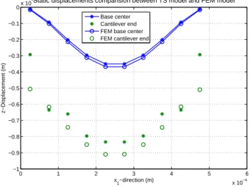
domain. . . 7 1.3 A two-dimensional view of (a) an array and (b) a cell . . . 7 1.4 Reference cell of AFM array . . . 9 1.5 Static displacements comparison between FEM model and two-scale

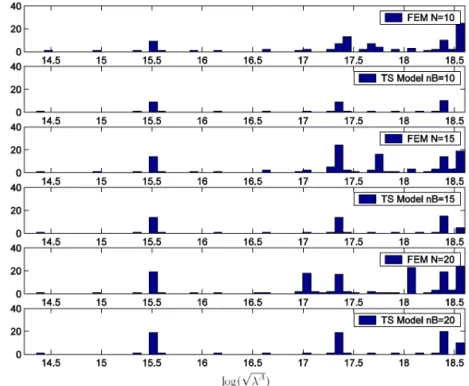
model with global modal decomposition. . . 24 2.1 Cantilever array without tips (a) and with tips (b). . . 31 2.2 Cantilever mode (a) and Base mode (b). . . 31 2.3 Distributions of log(√λA) of the FEM model and of the two-scale

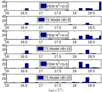
model . . . 32 2.4 Eigenvalue density comparison for N = 3, 4 and 5 . . . 33 2.5 Eigenvalue density comparison for N = 10 . . . 33 2.6 The ﬁrst base mode of (a) FEM model and (b) Two-scale model.

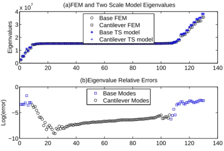
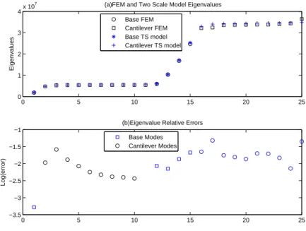
The ﬁrst cantilever mode of (c) FEM model (d) Two-scale model . 34 2.7 (a) Eigenvalue density distributions and (b) its relative errors for

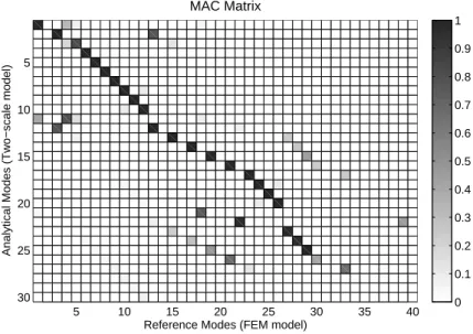
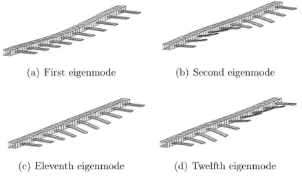
the FEM model and for the two-scale model . . . 35 2.8 MAC matrix between the two-scale model modes and the FEM modes 37 2.9 Eigenmode shapes of (a) φA

1,1, (b) φ

ref

1 , (c) φA2,2, (d) φ

ref

13 . . . 38

2.10 (a) Superimposed √λA of the two-scale model with a selection of those of the finite element model, (b) Errors in logarithmic scale . . 38 2.11 First-order finite difference sensitivity analysis . . . 39 2.12 Eigenmodes of the two-scale model . . . 40

(19)

2.13 Displacement of a 10-cantilever array under a static load of (a)

Two-scale Model (b) FEM model . . . 41

2.14 Displacement comparison of static analysis of 10-cantilever array at ﬁfth cantilever . . . 41

2.15 Displacement at (a) sixth cantilever end, and (b) ninth cantilever end in dynamic regime . . . 42

2.16 A one-dimensional view of (a) an Array and (b) a Cell . . . 46

2.17 One-dimensional arrays of AFM. Courtesy of André Meister and of Thomas Overstolz, CSEM Neuchâtel Switzerland. . . 46

2.18 (a) Side view and (b) Top view of a reference cell . . . 46

2.19 First-order ﬁnite diﬀerence sensitivities . . . 49

2.20 Parametric analysis of active design parameters and features (a) S_Tapex (b) S_Spring . . . 50

2.21 Scatter plots of Monte Carlo sampling . . . 51

2.22 Principal component analysis . . . 51

2.23 Evolution plot by solving mono-objective optimization problem . . 52

2.24 Pareto plot of Monte Carlo sampling between (a) F_Gapcell and C_FP and (b) F_Gap and C_base . . . 53

2.25 Uncertainty qualiﬁcation analysis . . . 54

2.26 Example of an optimized design geometry. The larger cantilevers with larger and higher tip situated in the corner of the probe array are used to land and adjust the probe array onto the sample surface. Courtesy of André Meister and Thomas Overstolz, CSEM Neuchâtel Switzerland. . . 55

3.1 AFM experimental setup . . . 58

3.2 A one-dimensional view of array of AFMs. . . 59

3.3 Intensity proﬁles: close to base-cantilever junction Θ∗₁ and above the tip of cantilevers Θ∗₂. . . 60

3.4 AFM arrays and samples. . . 66

3.5 Estimated sample topography with Formula (3.9). . . 67

3.6 Estimated sample topography after phase correction. . . 67

3.7 (a) One surface viewed in three-dimensional (b) Stitched surface . . 68

4.1 One component of the function k(λ) . . . 74

4.2 The contour in the Cauchy integral formula . . . 75

4.3 Analog computation of Λhv1.. . . 77

4.4 Five adjacent interior cells. . . 77

4.5 Four boundary cells. . . 78

4.6 Analog computation of the k-th equation (4.13). . . . 79

(20)

B.1 The main interface of the software AFMALab. . . 92

B.2 Menu of Project in AFMALab . . . 93

B.3 Menu of Model in AFMALab . . . 94

B.4 Material parameter settings. . . 94

B.5 Load settings ﬁle . . . 95

B.6 Menu of Compute in AFMALab . . . 95

B.7 Menu of Plots in AFMALab . . . 96

B.8 (a) 2D plot and (b) 3D plot of static analysis. . . 97

B.9 Mode plot of modal analysis. . . 97

B.10 Menu of Optimization in AFMALab . . . 98

B.11 Main interface of SIMBAD. . . 99

(21)

(22)

2.1 List of log( √

λA_ij) of the two-scale model . . . 36 2.2 L2_{-norm error for diﬀerent loads} _{. . . .} ₄₁

2.3 Ratios of the displacements at the free end of cantilevers to this of a loaded one in static regime . . . 42 2.4 Ratios of maximum displacements at the free end of cantilevers to

this of a loaded one under ﬁrst base eigenfrequency excitation . . . 43 2.5 Ratios of maximum displacements at the free end of cantilevers to

this of a loaded one under ﬁrst cantilever eigenfrequency excitation 44 2.6 List of design parameters . . . 47 2.7 Design features . . . 48 2.8 Design objectives . . . 48 2.9 Nonlinear design constraints . . . 49 2.10 Designs of probe arrays deﬁned using the design decision making

tool SIMBAD. The values in italic correspond to the initial condi-tions, and the values in bold to the optimized design parameters.. . 55

(23)

(24)

ℓ0

C The cantilever width in the reference cell, page 10 ϵ The inverse of dilatation of any cell, page 8

γ_R,O The tip-object interface, page 13

λA The eigenvalue of system, page 16

λB The macroscopic eigenvalue of base, page 17

λC The microscopic eigenvalue of cantilever, page 17

LB _{The linear operator, page 12} µ The array size, page 8

ν Poisson coeﬃcient, page 88

ω The ﬁlled rectangle covering the full array, page 8

bu The inverse two-scale transform applied to two-scale transform of u, page 9

uA _{The approximation of u in the physical system, page 9}

v The approximated inverse for the two-scale transform of v , page 8

ψA The eigenvector of system, page 16

ρB The eﬀective surface mass of base, page 10

σαβ The plane stresses, page 88 ε The cell size, page 8

ε∗ The ratio of the cell size ε, page 8

(25)

φC _{The microscopic eigenvector of cantilever, page 17}

bv The two-scale transform applied to inverse two-scale transform of v, page 9 buϵ _{The two-scale transform of u(x), deﬁned for any} _{ex and for any y, page 8}

ex The two ﬁrst components of moments (x1, x2) of x, page 9

ey The two ﬁrst components of moments (y1, y2) of y, page 9

ζ The tip-object friction coeﬃcient, page 13

E Young modulus, page 88

EC _{The cantilever elastic modulus, page 12} fB _{The base eﬀective load per unit area, page 13} FC0 The load per unit length of cantilevers, page 10

FC _{The cantilever two-scale load per unit area times area in ω}_{× e}_Y

C, page 13 FD The two-scale load corresponding to a periodic distribution of concentrated

load applied at points zc_{= x}c_{+ ϵy}0_{, page 13}

FO The object two-scale load per unit area times volume, page 13

FR0 _{The vector comprised of eﬀective forces and moments of rigid part, page 11} FR _{The tip two-scale load per unit area times area in ω}_{× e}_Y

C, page 13 GC _{The cantilever two-scale moment per unit area times area in ω}× e_Y

C, page 13 GD _{The two-scale moment corresponding to a periodic distribution of}

concen-trated load applied at points zc _{= x}c_{+ ϵy}0_{, page 13}

GR _{The tip two-scale moment per unit area times volume in ω}_{× e}_Y

C, page 13 g_αB The the base eﬀective moments about the plate section per unit area,

page 13

h The thickness of plate, page 12

hB The thickness of base, page 10 hC The thickness of cantilever, page 10

(26)

M The shear force matrix in base, page 14

mC0 The linear mass density of cantilevers, page 10

MC _{The shear force matrix in cantilevers, page 14}

mC The two-scale mass density in cantilever per unit area times area , page 13

nB _{The number of base modes, page 23} nC _{The number of cantilever modes, page 23}

RB _{The homogenized stiﬀness tensor of base, page 10}

rB _{The two-scale stiﬀness tensors per unit area in ω and per unit area in base}

e

YB, page 12

rC0 _{The linear stiﬀness coeﬃcient of cantilevers, page 10}

rC The two-scale stiﬀness tensors per unit area in ω and per unit area in can-tilever eYC, page 12

RP _{The thin plate stiﬀness per unit area, page 12} sαβ The strains, page 87

t The time variable, page 10

uA _{The two-scale approximation of u, page 8}

uP The elastic displacements in the model of a Kirchhoﬀ-Love thin plate inter-acting with objects, page 87

u0₃ Initial transverse displacement, page 14

u1

3 Initial velocity, page 14

uA

3 The third component of the vector of mechanical displacement, page 10

u0_α Initial lateral displacements in objects, page 14

u1

α Initial velocity in objects, page 14 xc The center of the cell, page 8

(27)

Y The ﬁlled reference cell, page 9

YB The base in a reference cell, page 9

YC The cantilever ﬂexible part in a reference cell, page 9 YO The object in a reference cell, page 9

YR The cantilever rigid part in a reference cell, page 9 YS The mechanical device in a reference cell, page 9

zF r The two-scale friction coeﬃcient at the two-scale tip-object interface ω ×

γ_R,O, page 13

AFM Atomic Force Microscope, page xii FEM Finite Element Method, page xii KCL Kirchhoﬀ Current Law, page xii LQG Linear Quadratic Gaussian, page xii LQR Linear Quadratic Regulator, page xii MAC Modal Assurance Criterion, page xii PCA Principal Component Analysis, page xii PDE Partial Diﬀerential Equation, page xii PDF Probability Density Function, page xii PNR Periodic Network of Resistances, page xii VCCS Voltage Controlled Current Source, page xii

(28)

Since its invention by [1], the Atomic Force Microscope (AFM) has opened new directions for a number of operations at the nanoscale with an impact in various sciences and technologies. A number of research laboratories are now developing large Arrays of AFM [2], [3] that can achieve imaging resolution similar to a single standalone AFM in parallel, (see Figure 1).

Figure 1: (a) optical image of a 4 ×17 probe array with SiN cantilevers anchored on parallel-beam base. The dark square at the end of each cantilever corresponds to the pyramidal shaped tip. (b) SEM images of a probe arrays with SiN can-tilevers anchored on a gridlike base. Courtesy of Centre Suisse d’Electronique et de Microtechnique (CSEM), Neuchâtel Switzerland.

The state-of-the art system that employs an array of cantilever probes is the Millipede device from IBM [4],[5],[6] designed for data-storage, but again, a number of new architectures are emerging, see [7], [8], [9], [10], [11], [12], [13], [14], [15]. For nanolithography applications, a two-dimensional probe array is utilized for dip pen nanolithography [16] and nanoprobe maskless lithography is reported in [17]. The main limitation of AFM devices is their low speed of operation and their low reliability. Thus, modeling and model based control of AFM employing a single cantilever probe has found extensive attention, (see M. Napoli [18], S.M. Salapaka et al. [19], M. Sitti [20] for instance). To improve the performance of AFM, an

H_∞ controller was employed in [21] and for AFM scanner in [22]. G. Schitter et al. [23] present a control strategy employing a model-based two-degrees-of freedom controller for high-speed topographical imaging. Regarding arrays, the group of

(29)

B. Bamieh, see [24] and the reference therein, has published a model of coupled cantilever arrays. It takes into account electrostatic coupling of cantilevers, and its derivation is phenomenological. In [25], both mechanical and electrostatic cou-pling neighboring cantilevers are modeled for an array of electrostatically actuated microcantilevers. In an array of cantilever probes, it is important to address the issue of cross-talk between cantilevers. Such cross-talk may have mechanical, ther-mal or electromagnetic origins and is an important eﬀect to be considered while designing the array.

We propose a simpliﬁed model for the elastic behavior of large cantilever two-dimensional arrays. It extends results in [26] by taking into account the dynamical regime instead of the static regime, and is applicable to two-dimensional arrays instead of to one-dimensional arrays. Moreover, it takes into account the possible interaction between AFM tips and sample being interrogated. A similar analysis for one dimensional array ignoring the interaction between the tip and the sample is reported in [27]. The detailed derivation of the results in [28], not yet reported, follows from the results in this thesis.

Our method is mainly based on a homogenization technique applicable to strongly heterogeneous materials or systems expressed in the framework of two-scale convergence (or approximation) as introduced in works of M. Lenczner [29], [30] or in D. Cioranesco, A. Damlamian and G. Griso [31]. In a preliminary step, its derivation also uses the asymptotic method for thin structures developed by P.G. Ciarlet [32] and of P. Destuynder [33]. We remark that the choice of a method for the modeling of the periodic array is not straightforward. Here, a standard ho-mogenization method is not applicable, where the local mechanical displacements of the moving parts may be of the same order as the displacements of the common support. Another aspect is that the lowest local eigenfrequencies of the moving parts are also in the same range of magnitude as those of the common support-ing base. These features are usual in many microsystems arrays. However, the homogenization method was developed for typical continuum mechanics applica-tions where the usual methods even with introduction of additional techniques has proven inadequate for modeling an array of micro-cantilever.

We review the main features of our simplified model. The array is comprised of cantilevers clamped in a common base, each possibly interacting with an object through its tip. We assume that the base is much stiffer than the cantilevers. This is expressed by saying that their stiffness have different asymptotic behaviors. The resulting model is composed of two evolution equations, one for the macroscopic behavior, related to the supporting base, and the other, at the microscopic level, which takes into account the cantilever dynamics. As required, their time scales are in the same range of magnitude and so are their mechanical displacements. We further assume that the tip is perfectly rigid, which is a commonly accepted

(30)

assumptions yield the general model. As an introduction, we also present a slightly simpler model, referred to as the Simple Model, for which we have carried numerical simulations and validations. It does not include possible interaction with objects and it neglects the width eﬀect in cantilevers.

For real-time control for arrays of microsystems like arrays of atomic force microscopes, micro-mirrors, or micro-membranes, we present a new approximation method based on the Simple Model. The microsystems are comprised of a very large number of units subjected to wanted or unwanted interactions (cross-talk eﬀect). Achieving global control of such a system remains a challenging task. Here, we propose a computational strategy with very ﬁne-grained computing processors allowing semi-decentralized exchanges, i.e. between neighbors only. We refer to this concept by using the term semi-decentralized architecture or computing.

In the past decade, a number of articles have focused on semi-decentralized distributed optimal control for systems with distributed actuators and sensors. Most of them deal with infinite length systems, see [34] and [35] for systems gov-erned by partial differential equations, and [36] for discrete systems. In articles [37] and [38] authors have introduced an approximation, for optimal control de-sign purposes, optimal control to a finite length beam endowed with a periodic distribution of piezoelectric sensors and actuators. Even-though here satisfactory results are obtained, it suffers from limitations of applying simple optimal control strategy, namely LQR, with simple control objective.

In [39] and [40], a comprehensive framework is introduced applicable to cover a large range of systems, with increased precision and robustness. The method is based on a general theory of optimal control for linear inﬁnite dimensional systems. It does not require that all operators involved are functions of a same operator in the system. They only need to be functions of this operator up to some change of variables. Regarding precision of our method, the Taylor series approximating a function of an operator has been replaced using the integral Cauchy formula from functional calculus followed by a quadrature rule for the contour integral.

A ﬁrst investigation for real-time vibration control of a one-dimensional can-tilever array has been carried out in the LQR framework. In view of real-time control applications, we have derived a Semi-Decentralized Approximation of the controller based on the two mathematical concepts of functional calculus and Dunford-Schwartz representation formula, and formulated its realization through PNR, see [41]. This Semi-Decentralized approximation method can be extended to other linear control theories, such as Linear Quadratic Gaussian (LQG) and

H_∞ control.

(31)

is the sensing system. Regarding sensing, in some cantilever arrays, the deflec-tion of cantilever is measured by piezoresistive sensor integrated in the cantilever. In [42], a cantilever arrays equipped with piezoresistive sensors was employed in liquid environment. However, this approach suffers from the complexity of the mi-crofabrication process of implementing the sensor in the cantilever. Additionally, the signal to noise ratio of piezoresistive arrays is limited due to the sensor noise. An interferometric readout method with imaging optics is provided in [43]. This approach does not suffer from optical cross-talk since the laser light reflected from one point on the cantilever is collected by only one pixel of the detector, and is in-dependent of the direction the reflected laser beam. However, interferometric data processing requires heavy computation due to the large number of cantilevers, which represents a barrier to rapid operation. Thanks to a new approach for deflection estimation of cantilever arrays through interferometry measurement in quasi-static regime, it is turning into reality for real-time estimation and control of cantilever arrays in the dynamic regime.

This dissertation is organized as follows. In chapter 1, we start by shortly in-troducing the Simple Model. We then formulate the general model precisely. The model implementation is detailed both for two-dimensional and one-dimensional cantilever arrays. The Base/Cantilever displacement decomposition of the

Sim-ple Model is also discussed. Chapter 2 addresses the verification of the simple model. The eigenvalues and eigenmodes of the simple model are compared to those obtained by a direct three-dimensional Finite Element Method (FEM) both for one-dimensional and two-dimensional cantilever arrays. The verification of the model in static and dynamic regime is also presented. To meet the design re-quirements of AFM arrays, an optimization tool is introduced with an illustrative example. The interferometry measurement for AFM arrays is presented in chapter 3. The least square algorithm for phase computation is provided. In chapter4, we present the semi-decentralized approximation method which is used LQR control and H_∞ filtering problem.

We draw our conclusion in chapter 5 with some remarks on future research work. A new software, AFMALab, for performing simulations for an array of cantilevers is presented in appendix B.

(32)

TWO-SCALE MODEL FOR

ARRAY OF CANTILEVERS

This chapter is devoted to the derivation of simple two-scale model in section1.1.1, and general two-scale model in section 1.1.2 for a two-dimensional array of can-tilevers. Each cantilever may be equipped with a rigid tip which can interact with the sample. For the simple model, we assume that there is no tip-sample inter-action and the variation of the displacement in the width direction of cantilevers is negligible. All these assumptions are not present in the general model. Here, cantilevers can be modeled by a classical Euler-Bernoulli beam equation and the motion of the base is governed by a Kirchhoﬀ-Love plate equation. The mathemat-ical proofs of the two-scale approximation technique are detailed in a submitted paper [28].

(33)

In section 1.2, we show the model implementation both for two-dimensional and one-dimensional array of cantilevers. At the end of this chapter, we propose a Base/Cantilever displacement decomposition of the simple model.

1.1 Model Description

We consider a two-dimensional array of cantilevers, (see Figure 1.1). It is

com-Figure 1.1: Array of Atomic Force Microscopes

prised of bases crossing the array in which cantilever are clamped. The bases are connected both in the x1-direction and in the x2-direction (see Figure 1.3 (a)),

so they constitute a single common support clamped on its external boundary. Cantilevers may be equipped with a rigid tip, as in Atomic Force Microscopes.

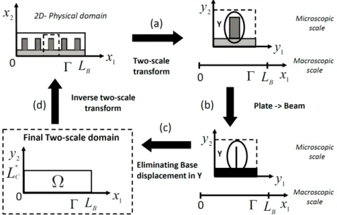
The two-scale model derivation steps are illustrated in Figure 1.2. First, (a) the two-scale transform (also called the unfolding operator) and the two-scale approximation are successively applied to map a thin plate model in bending from the physical domain to a two-scale domain comprised of a reference cell and the macroscopic domains. Then, (b) the displacement variation in the width direction of cantilevers is neglected. In (c), base displacements in the reference cell are explicitly calculated and eliminated to yield the model in the so-called two-scale

domain where the optimal control is implemented. Finally, (d) an inverse

two-scale transform technique is applied to map the solutions in the two-two-scale domain back to the physical domain.

The whole array can be viewed as a periodic repetition of a same cell, in the two directions x1 and x2, (see Figure 1.3 (a)).

(34)

Figure 1.2: Two-scale transform and inverse two-scale transform in two-scale do-main

Figure 1.3: A two-dimensional view of (a) an array and (b) a cell

We suppose that the numbers of rows and columns of the array are suﬃciently large, namely larger or equal to 10. The simpliﬁed model will be an approximation of the full model in the sense of small values of ε∗, the ratio of the cell size ε, to

(35)

array size µ, i.e.

ε∗ = ε/µ. (1.1)

To build it, we shall make use of the two-scale approximation that we brieﬂy introduce. Consider any point x = (x1, x2, x3) of the three-dimensional space is

decomposed as

x = xc+ ϵy,

where xc_{represents the coordinates of the center of the cell of x, ϵ =}

  ε ∗ ₀ ₀ 0 ε∗ 0 0 0 1  , and y = ϵ−1(x−xc_{) is the dilated relative location of x with respect to x}c_{. In current}

cell, the points are identiﬁed by determining the cell in which the points (x1, x2) lie

(see Figure1.3 (a)). Then, points with coordinates y vary in the unique so-called

reference cell, that is obtained through a translation and the dilatation ϵ−1 of any current cell, (see Figure1.3 (b)) for a two-dimensional view of the reference cell.

Now, considering a distributed ﬁeld u(x), we introduce its two-scale transform buϵ₍_{ex, y) = u(x}c_{+ ϵy),}

deﬁned for any ex = (x1, x2) belonging to the two-dimensional ﬁlled section of

the cell, centered at xc_{= (x}c

1, xc2, xc3), and for any y = (y1, y2, y3) varying over the

reference cell. We emphasize that through this construction ex varies in a filled rectangle covering the full array, which we refer to as ω. By construction, the two-scale transform is constant, with respect to its first variable ex, over each cell. Since it depends on the ratio ε∗, it may be approximated by the asymptotic field,

denoted by uA_{, obtained when ε}∗ _{approaches (mathematically) 0:}

buϵ _{= u}A_{+ O(ε}∗_).

The approximation uA is called the two-scale approximation of u. We mention that as a consequence of the asymptotic process, the partial function ex 7→ uA₍_{ex, .)}

is continuous unlike the map ex 7→ buϵ₍_{ex, .).}

Now, we observe that uA₍ex, y) is a two-scale ﬁeld, and therefore cannot be

directly used as an approximation of the ﬁeld u(x) in the real array of cantilevers. So, an inverse two-scale transform must be applied to uA_{. However, since} _{ex 7→} uA₍ex, y) is continuous, uA_{does not belong to the range of the two-scale transform.}

Hence we introduce an approximated inverse for the two-scale transform,

(36)

in the sense

bu = u + O(ε∗_{) and b}_{v = v + O(ε}∗_),

for sufficiently regular functions u(x) and v(ex, y). We are led to make two different choices for x 7→ v(x), when x belongs to a cell centered at xc. The first

one applies to x belonging to a cantilever,

v(x) = ⟨v(., ϵ−1(x− xc))⟩_ex,

it is a mean in ex over the cell. The other is for x in the base,

v(x) = v(., ϵ−1(x− xc)).

Once an approximate inverse two-scale transform is deﬁned, we retain uA _as

our approximation of u in the physical system. In the dissertation, we apply this technique to the mechanical displacements in the array, and we derive the equations governing the resulting two-scale ﬁeld uA_.

Notations The reference cell is divided into the mechanical device YS and the

object YO. Furthermore, the device YS is divided into the base YB, the cantilever

ﬂexible part YC, and the cantilever rigid part YR, (see Figure 1.4). The ﬁlled

reference cell Y is a rectangle parallelepiped in R3_.

Figure 1.4: Reference cell of AFM array

We will use the tilde notation on variables x or y to refer to their two ﬁrst com-ponents, ex = (x1, x2) and ey = (y1, y2) where x = (x1, x2, x3) and y = (y1, y2, y3).

Accordingly, we will use the in-plane gradient∇_ey= (∂y1, ∂y2), the in-plane Laplace

operator ∆_ey= ∂_y2₁_y₁+∂_y2₂_y₂, the in-plane unit outward external normal components

n_ex= (nx1, nx2) and ney= (ny1, ny2) to the boundary of ω and of the reference cell.

The in-plane section of the reference cell Y is refereed as eY when the sections of

(37)

used for their interfaces and for boundaries. The inverse of the cell section surface is constantly used, so it is referred to as

eκ = 1

|eY|. (1.2)

The jump of a ﬁeld v at an interface γ is written as [[v]]γ. Finally, we use the

operation ” : ” for the inner product between two matrices A and B of same dimensions, A : B =∑_i,jAijBij.

1.1.1 The Simple Two-Scale Model

Our models are formulated from the Kirchhoﬀ-Love thin plate model of the whole structure, and we will always assume that the ratio of cantilever thickness hC to

base thickness hB is small, namely hC hB

≈ ε∗4/3_. _(1.3)

Applying the two-scale approximation technique to the third component of the vector of mechanical displacement ﬁelds yields uA₃(t,ex, y) where t represents the time variable and is treated as a parameter. In the following, we detail the equations governing uA

3, all parameters of its model being stated in section 1.1.2.

From the analysis, it appears that uA₃ is independent of y3 everywhere. In

the Simple Model, we consider cantilevers made of an isotropic material and there variations of y1 7→ uA3(t,ex, y) are neglected. So their motions are governed by a

classical Euler-Bernoulli beam equation in the microscopic space variable y2,

mC0∂_tt2uA₃ + rC0∂_y4₂_...y₂uA₃ = FC0, (1.4) with mC0 _{their linear mass density, r}C0 _{their linear stiﬀness coeﬃcient, and} FC0 _{their load per unit length, see (}_1.17_{), (}_1.13_{), (}_1.21_{).] This model holds for all}

ex = (x1, x2), and therefore represents motions of an inﬁnite number of cantilevers

parameterized by ex and y capture the relative motion with respect to this. For y varying along the base, y 7→ uA

3(t,ex, y) is constant and there the

dis-placement uA₃(t,ex) is governed by a Kirchhoﬀ-Love plate equation

ρB∂_tt2uA₃ + div_ex(div_ex(RB :∇_ex∇T_exu₃A)) + ℓ0_CrC(∂3_y₂_y₂_y₂uA₃)_|junction= fB, (1.5) where ρB_{, R}B_{, R}B _{and ℓ}0

C are respectively its eﬀective surface mass, its

homog-enized stiﬀness tensor, its eﬀective load per unit surface, and the cantilever width in the reference cell, see (1.15), (1.14), (1.18). The term rC(∂_y3₂_y₂_y₂uA₃)_|junction is a distributed load originating from shear forces exerted by cantilevers on the base at base-cantilever junctions.

(38)

At base-cantilever junctions, a cantilever is clamped in the base, so

uA₃_|cantilever = uA₃_|base and ((∂y1, ∂y2)u

A

3.(n1, n2)T)|cantilever = 0, (1.6)

because ∇yuA3 = 0 in the base. Other cantilever ends may be free with equations,

∂_y2 2y2u A 3 = 0 and ∂ 3 y2y2y2u A 3 = 0, (1.7)

or may be equipped with a rigid part (usually a tip in Atomic Force Microscopes), then JR∂tt ( uA 3 ∂y2u A 3 ) + rC0 ( −∂3 y2y2y2u A 3 ∂2 y2y2u A 3 ) = FR0 (1.8) at a junction between an elastic part and a rigid part. Here, JR _{is a matrix of}

moments and FR0 is comprised of eﬀective forces and moments stated in (1.32). Last, the external base boundary being clamped in a ﬁxed support

uA₃ = 0 and∇_exuA₃.n_ex = 0 (1.9) on its boundary.

1.1.2 The General Two-Scale Model

In section 1.1.1, the model was introduced assuming that the base and cantilevers are rectangle parallelepiped, and that their deformations in the y1 direction are

negligible. Now, we relax these assumptions, and we present in detail a more gen-eral two-scale model that may also take into account possible interactions between tips and rigid objects. We restrict the presentation to the situation where the bodies are in contact with friction. This is applicable to contact mode microscopy with atomic force microscopes. In addition to approximation of displacements, we provide approximations of elastic strains and stresses. The approximations are still posed in the Kirchhoﬀ-Love thin plate model where we still neglect mean (in the thickness direction) in-plane displacements.

Model Parameters The model parameters result from two-scale approxima-tions of the physical data, namely coeﬃcients, loads and initial condiapproxima-tions.

Remark 1 It is natural to consider that the problem geometry and equation

coef-ficients are parameterized by ε∗, but it is artificial to say the same thing regarding other data as loads or initial conditions. However, to follow the common use we proceed as if they were also known sequences of ε∗, with a known two-scale approx-imation. For some of them, we do not require their direct two-scale approximation but this of their product by a power of ε∗. This provide a measure of the asymptotic behavior required so that the model be well justified. Remark that for actual model computations, we do not use the two-scale approximation of parameters but only their two-scale transform.

(39)

Let RP _{be the thin plate stiﬀness per unit area, for instance for a plate with}

thickness h made of an isotropic material

RP_αβγρ = Eh

3

12(1 + ν)(

ν

1− νδαβδγρ+ δαγδβρ), (1.10) the assumption (1.3) on ratio thicknesses may be restated with respect to stiﬀ-ness as RP |ΩC RP |ΩB ∼ ε∗4_. _(1.11)

Posing the order of magnitude of base stiﬀness in the range of 1 with respect to

ε∗, the two-scale stiﬀness tensors rB (respectively rC) per unit area in ω and per unit area in the base eYB (respect. in cantilever eYC) is deﬁned as the two-scale

approximation of eκRP _{(respect. of ε}∗−4eκRP_{), that we write simply as,}

rB ≈ eκ bRP in ω× eYB (respect. rC ≈ ε∗−4eκ bRP). (1.12)

The stiﬀness per unit area in ω and per unit length in cantilever of the Simple

Model is therefore rC0 = ℓ0_C(1 − ν2)rC, where we recall that ℓ0_C is the scaled cantilever width ℓC/ε∗ in the reference cell. In case of an isotropic material,

rC0 ≈ ε∗−4eκℓ0_CECIC = ε∗−4eκECh

3

Cℓ0C

12 , (1.13)

EC _{being the cantilever elastic modulus and I}C _{= h}3

C/12 the second moment

of cantilever section. We introduce the effective stiffness tensor RB per unit area in the base, RB_αβγρ= ∫ e YB r_αβγρB + r_αβξζB LB_ξζγρ dey, (1.14) where the tensorLB _{is defined in (}_A.6_{) below. Then, ρ representing the volume}

mass density, the eﬀective mass density ρB _{per unit area in the base is} ρB≈ eκ

∫

YB

bρ dy in ω. (1.15)

The other mass densities appearing in the model are two-scale densities: in cantilever mC _{is per unit area times area when in the rigid tips and in objects ρ}R

and ρO are per unit area times volume. Indeed,

mC ≈ eκ

∫ hC/2

−hC/2

(40)

The two-scale mass density mC0 _{per unit area in ω and per unit length in}

cantilevers follows,

mC0 = ℓ0_CmC. (1.17) The base eﬀective load fB _{per unit area, the base eﬀective moments g}B

α about

the plate section per unit area are derived from the two-scale approximations of the vector of loads f = (f1, f2, f3) per unit volume,

fB ≈ eκ

∫

YB

b

f3 dy, and gαB≈ eκ

∫

YB

y3fbα dy in ω. (1.18)

The cantilever two-scale load FC _{and the moment G}C _{per unit area times area}

in ω × eYC, the tip two-scale load FR and the moment GR per unit area times

volume, and the object two-scale load FO per unit area times volume are deﬁned similarly from f FC ≈ eκ ∫ hC/2 −hC/2 b f3 dy3 and GCα ≈ eκ ε∗ ∫ hC/2 −hC/2 y3fbα dy3 in ω× eYC, (1.19) FR≈ eκ bf3, GRα ≈ eκ ε∗y3fbα in ω× YR and F O _{≈ ε}∗_{eκ b} f in ω× YO. (1.20)

The cantilever two-scale load of the Simple Model follows

FC0 = ℓ0_CFC. (1.21) The two-scale load and moment corresponding to a periodic distribution of con-centrated load (∑_cfciδzc(x))_i=1..3 applied at points zc= xc+ ϵy0 is

FD = 1 (ε∗)d ∑ c χ_Y_eε_(xc₎(z)fcδy0(y)≈ |eY| ∑ c δ_exc(z)f_cδ_y0(y) (1.22) and GD = 1 (ε∗)d+1 ∑ c χ_Y_eε_(xc₎(z)fcy30δy0(y)≈ |e Y| ε∗ ∑ c δ_exc(z)f_cy0₃δ_y0(y).

The two-scale friction coeﬃcient at the two-scale tip-object interface ω× γ_R,O is an approximation built from the tip-object friction coeﬃcient ζ,

zF r≈ eκ bζ

ε∗2. (1.23)

For given initial transverse displacement u0

3 and velocity u13 in the whole system

together with lateral displacements u0_α and velocity u1_α in objects, the two-scale initial displacements and velocities are deﬁned by the approximations

uA0₃ ≈ bu0₃, uA1₃ ≈ bu1₃ in ω× (YS∪ YO),

(41)

Moreover, uA0 _{and u}A1 _{are assumed to fulﬁl the forthcoming kinematics (}_1.24 -1.28).

Admissible kinematics The two-scale ﬁelds uA _{satisﬁes a kinematics}

inher-ited from the Kirchhoﬀ-Love kinematics and from the two-scale approximation of derivatives. In the whole mechanical structure comprised of a base and of can-tilevers,

uA₃ and uB are independent of y3. (1.24)

We neglect mean in-plane displacements, and we assume that the surface y3 = 0

corresponds to the mean section of the cantilevers and of the base. So,

uA_α =−y3∂xαu A 3 in ω× YB and uAα =−y3∂yαu A 3 in ω× (YC∪ YR). (1.25) In the base, uA 3 is independent of (y1, y2), that is ∇eyuA3 = 0. (1.26)

The conditions of rigidity for tips and for objects are formulated as

∇ey∇TeyuA3 = 0 in tips and sy(uA) = 0 in objects, (1.27)

where sy(u) = 1₂(∇yu + (∇yu)T) is the usual strain tensor in the y variables. The

contact condition between tips and rigid objects results in normal displacement continuity through their interface γ_R,O,

[[uA]]γR,O.ny = 0, (1.28)

where ny denotes the unit outward normal vector to boundaries in the reference

cell.

Equations of motion In cantilevers, the transverse displacement uA

3 is

gov-erned by a Love-Kirchhoﬀ thin plate equation in the y variables,

mC∂_tt2uA₃ + div_ey(div_ey(MC(uA₃))) = FC in ω× eYC, (1.29)

and the shear force matrix in cantilevers is MC_(uA

3) = rC : ∇ey∇

T

eyuA3. In

the base, the transverse displacement uA₃ is also governed by a thin plate Love-Kirchhoﬀ model in the macroscopic variables, with a contribution of the bending moment exerted by the cantilever distribution. This coupling with cantilevers appears under the form of an integral along the interface line eγ_B,C between eYB

and eYC, ρB∂_tt2uA₃ + ∂_x2_α_x βM B αβ(u A 3)− ∫ eγB,C div_ey(MC(uA₃)).n_eydes = fB in ω× eYB, (1.30)

(42)

where the shear forces in the base are given by

M_αβB(uA₃) = RB_αβγδ∂_x2_γ_x_δuA₃.

For the sake of shortness, we write the motion equations in tips and in objects under their variational formulation. This avoids formulating in detail their dynamics together with the interface condition. The admissible displacement set is built from the above admissible conditions,

WA={uA deﬁned in YR∪ YO satisfying (1.24, 1.25, 1.27, and 1.28)}.

For a given vector ﬁeld v ∈ WA_{, we introduce its tangent component v}

T on the

interface γ_R,O deﬁned as,

vT = v− (v.ny)ny,

and eγ_C,R the interface between eYC and eYR. The linear form of the right hand side

is lR(v) = ∫ YR F₃Rv3− GR.∇eyv3 dy + ∫ YO FO.v dy− ∫ eγC,R GC.n_ey v3 des,

and the bilinear forms are

cR(uA, v) = ∫ YR ρRuA₃v3 dy + ∫ YO ρOuA.v dy, bR(uA, v) = ∫ γR,O

zF r[[uA_T]]γ_R,O.[[vT]]γ_R,O ds aR(uA₃, v3) =

∫

eγC,R

(MC(uA₃)n_ey).∇_eyv3− divey(MC(uA3)).neyv3 des.

The variational formulation states as uA_{(t, x, .)}_{∈ W}A _and

∂_tt2cR(uA, v) + ∂tbR(uA, v) + aR(uA3, v3) = lR(v) for all v ∈ WA. (1.31)

For the Simple Model, this equation was restated as a boundary condition (1.8) at eγC,R where JR= ( J0 J1 J1 J2 ) and FR0= ( ∫ YRF R 3 dy− ℓ0CGC_|eγ_C,R ∫ YRF R 3 (y2− y2|eγ_C,R) dy− GR2 ) , (1.32) with Jk = ∫ YR(y2− y2|eγC,R) k _dy

2 being a kth moment of the rigid part YR about the

junction eγ_C,R in the direction y2.

Interface and boundary conditions Cantilevers being clamped in a base, the deﬂection uA₃ and its derivatives are continuous through the base-cantilever interface eγ_B,C, uA₃_{|ω× e}_Y C = u A 3|ω×eYB and (∇eyu A 3)_{|ω× e}YC = 0 at eγB,C. (1.33)

(43)

At free cantilever boundaries,

nT_eyMC(uA₃)n_ey= 0, ∇_ey(nT_eyMC(uA₃)τ_ey).τ_ey+ div_ey(MC(uA₃)).n_ey= 0 (1.34) where τ_eyis the tangent vector to the reference cell’s boundary. Along the complete boundaries of ω where base is clamped, the two-scale transverse displacement fulﬁls clamping like conditions,

uA₃ =∇_exu₃A.n_ex = 0 at ∂ω× eYB. (1.35)

Initial conditions The two-scale transverse displacement and its velocity are initialized in the whole system ω× (YS∪ YO) by

uA₃ = uA0₃ , ∂tuA3 = u

A1

3 .

In-plane displacements and their time derivatives are initialized, in objects ω× YO

only, by

uA_α = uA0_α and ∂tuAα = u A1

α . (1.36)

Eigenvalue Problem We consider the model without object, and we state the associated eigenvalue problem as well as a property of factorization of eigenvectors. An eigenvalue λA and an eigenvector ψA(ex, ey) satisfy the constraints

∇eyψA= 0 in eYB, ∇ey∇T_eyψA= 0 in YR, (1.37)

an equation in the base

div_ex(div_ex(MB(ψA)))− ∫ eγB,C div_ey(MC(ψA))_{| e}_Y C.ney ds = ρ B_λA_ψA _{in ω}_{× e}_Y B, (1.38) an equation in cantilevers div_ey(div_ey(MC(ψA))) = λAmCψA in eYC, (1.39)

and a variational formulation in the rigid part,

ψA_|Y_R ∈ WA, aR(ψA, v) = λAcR(ψA, v) for all v ∈ WA, (1.40) endowed with the reduced deﬁnition

WA ={v deﬁned in YR | ∂y3v = 0 and∇ey∇

T

eyv = 0}.

The boundary and interface conditions for ψA are not detailed since they are the same as for uA

(44)

Factorization of the Eigenvectors Now, we state that each eigenvector ψA can be written as the product of a macroscopic eigenvector defined in ω only by a microscopic (or local) eigenvector defined in eYC ∪ YR only. We first introduce

the macroscopic eigenvalue problem where λB and φB₍ex) denote respectively an

eigenvalue and an eigenvector,

div_ex(div_ex(MB(φB))) = λBρBφB in ω,

φB =∇_exφB.n_ex= 0 on ∂ω.

Then, for each λB we deﬁne the microscopic eigenvalue problem in cantilevers where λC and φC _{represent an eigenvalue and an eigenvector,}

div_ey(div_ey(MC(φC))) = λCmCφC in eYC,

λBρBφC − div_eyMC(φC)n_ey= λCρBφC and ∇_eyφC = 0 at eγ_B,C,

and nT_eyMC(φC)n_ey= 0,

∇ey(nTeyMC(φC)τey).τey+ divey(MC(φC)).ney= 0 at free boundaries,

together with the variational formulation in rigid parts,

φC_|Y

R ∈ W

A_{, a}R_(φC_{, v) = λ}C

cR(φC, v) for all v ∈ WA.

Finally, we state the decomposition property. For the sake of brevity its proof is omitted.

Proposition 2 For each pair (λA, ψA) solution to (1.37-1.40), there exists a unique pair (λB, φB_{) and a unique pair (λ}C_{, φ}C_{) such that ψ}A₍_{ex, ey) = φ}B₍_ex)φC₍_{ey) and} λA = λC. Reciprocally, for any pair (λB, φB_{) and any pair (λ}C_{, φ}C_{), its} combi-nation (φB(ex)φC(ey), λC) determines the pair (ψA(ex, ey), λA) which is solution to

(1.37-1.40).

1.2 Model Implementation

In this section, we provide further details in view of the model implementation for a two-dimensional array and then for a one-dimensional array without object.

(45)

First, we summarize the coeﬃcient expressions in case of constant coeﬃcients ℓ0_C = ℓC ε∗, L 0 C = LC ε∗ , eκ = 1 |eY|, R P αβγρ= Eh3 12(1 + ν)( ν 1− νδαβδγδ+ δαγδβρ), rB ≈ eκRP in ω× eYB, rC = (1− ν2)rC1111 = ε∗−4 eκEh3 12 , RB_αβγρ= ∫ e YB r_αβγρB + r_αβξζB LB_ξζγρ dey, ρB≈ eκ|YB|ρ_|Y_B, mC ≈ eκhCρ_|Y_C, ρR≈ eκρ_|Y_R, Q = N ( J0 J1 J1 J2 ) N, with N = ( 1 0 0 1/L0_C ) and Jk = ∫ YR (y2− L0C)k dy, fB ≈ eκ ∫ YB b

f3 dy, and gαB ≈ eκ

∫ YB y3fbα dy in ω, FC ≈ eκ ∫ hC/2 −hC/2 b f3 dy3 and GC₂ ≈ eκ ε∗ ∫ hC/2 −hC/2 y3fb2 dy3 in ω × eYC, FR≈ eκ bf3, GRα ≈ eκ ε∗y3fbα in ω× YR.

1.2.1 The Two-dimensional Case

We detail the formulation of the model when variations of displacements in can-tilever width are ignored. We recall that uA

3 is solution of the problem: Find

uA

3 ∈ V3A such that

∂_tt2cA(uA₃, vA₃) +eaA(u₃A, v₃A) = lA(vA₃) for all v₃A∈ V₃A (1.41) accompanied with initial conditions

uA₃ = uA0₃ and ∂tuA3 = u A1 3 at t = 0, where eaA_(uA 3, v3A) = ∫ ω[ ([ RB _:_∇ ex∇TexuA3 ] :∇_ex∇T_exvA 3 ) | eYB +ℓ0 C ∫L0_C 0 rC∂ 2 y2y2u A 3∂y22y2v A 3 dy2C]dex, (1.42) cA(uA₃, v₃A) =∫_ω[(ρBuA₃v₃A)_{| e}_Y B + ℓ 0 C ∫L0 C 0 m C_uA 3v3A dyC2 +∫_Y Rρ R_uA 3v3A dy]dex, (1.43) and lA_(vA 3) = ∫ ω[(f B_vA 3 − gB.∇exv3A)_{| e}YB + ∫ e YCF C _vA 3 − GC2∂y2v A 3 dey +∫_Y RF R_vA 3 − GR2∂y2v A 3 dy]dex + (FD − GD)v3A. (1.44) The eigenmodes ψA∈ VA 3 are solution of eaA_(ψA_{; v}A 3) = λ A_cA_(ψA_{, v}A 3) for all v A 3 ∈ V A 3 (1.45)

(46)

with the normalization condition cA_(ψA

, ψA) = 1.

For a rectangle domain ω = (0, L1)× (0, L2), we introduce the factorization of

ψA(ex, y2) = φB(_Lx1₁,_Lx2₂)φC(

yC

2

L0

C

) where φB _{and φ}C _{are solution to the two following}

eigenvalue problems where yC

2 is the translation of y2 equal to zero at the clamping

point of the cantilever to the base. First, φB ∈ H₀2((0, 1)2) with λB are solution to the weak formulation

aB_(φB_{, v}B_{) = λ}B

cB_(φB_{, v}B_{) for all v}B ∈ H2

0((0, 1)2)

normalized by the condition cB(φB, φB) = 1, (1.46) where the bilinear forms are deﬁned on the scaled domain (0, 1)2 _by

aB(φB, vB) = ∫_(0,1)2 [ RB0 :∇ξ∇T_ξφB ] :∇ξ∇T_ξvB dξ and cB(φB, vB) =∫_(0,1)2φ B _vB _dξ, (1.47)

and RB0 _{is the scaled homogenized stiﬀness tensor} RB0 αβγδ = RB αβγδ RB maxL0αL0βL0γL0δ with L0 α = Lα µ , µ = L1+L2 2 and R B max= maxα,β,γ,δ(RBαβγδ). (1.48) Next, φC _{∈ V}C ₌ _{{v ∈ H}4_{(0, 1)} _{| ∂}

ξv(0) = 0} with λC are solution to the weak

formulation aC(φC, vC) = λCcC(φC, vC) for all vC ∈ VC normalized by cC_(φC_{, φ}C_{) =} rC (L0 C)4mC , (1.49) where aC(φC, vC) = |ω|R B max µ4 λ B( φC vC)_|ξ=0+ |ω|ℓ 0 C (L0 C)3 ∫ 1 0 rC_∂2 ξξφC∂ξξ2 vC dξ, (1.50) and cC_(φC_{, v}C_{) =} |ω|rC (L0 C)4mC [(ρB_φC_vC₎ |ξ=0+ ℓ0CL0C ∫1 0 m C_φC_vC _dξ +ρR∫ YRφ C_vC _dy]. (1.51)