2011 — Implementation and validation of a method for computing the induced drag of multiple lifting surfaces aircrafts

ÉCOLE DE TECHNOLOGIE SUPÉRIEURE UNIVERSITÉ DU QUÉBEC

MEMORANDUM PRESENTED TO ÉCOLE DE TECHNOLOGIE SUPÉRIEURE

IN PARTIAL FULFILMENT

OF THE REQUIREMENTS FOR A MASTER’S DEGREE IN MECHANICAL ENGINEERING

M.Eng.

BY

Antoine MOREAU

IMPLEMENTATION AND VALIDATION OF A METHOD FOR COMPUTING THE INDUCED DRAG OF MULTIPLE LIFTING SURFACES AIRCRAFTS

MONTREAL, AUGUST 9 2011 Copyright 2011 reserved by Antoine Moreau

BOARD OF EXAMINERS

THIS THESIS HAS BEEN EVALUATED BY THE FOLLOWING BOARD OF EXAMINERS

Mr. Azzeddine Soulaïmani, Thesis Supervisor

Department of Mechanical Engineering at École de Technologie Supérieure

Mr. Éric Laurendeau, Thesis Co-supervisor

Advanced Aerodynamics Department of Bombardier Aerospace

Mr. Hany Moustafa, President of the Board of Examiners

Department of Mechanical Engineering at École de Technologie Supérieure

Mr. Wahid Ghaly, External Examiner

Department of Mechanical and Industrial Engineering at Concordia University

THIS THESIS HAS BEEN PRESENTED AND DEFENDED BEFORE A BOARD OF EXAMINERS AND PUBLIC

AUGUST 9 2011

ACKNOWLEDGMENT

This project was rendered possible with the collaboration of École de Technologie Supérieure and Bombardier Aerospace Company into a new Masters program in Québec; the BMP bursaries, which allowed students to complete a Master’s degree while working for, and inside a company which inspired them. I can consider myself lucky to have been chosen for this new program. I would like to thank Eric Laurendeau from Bombardier’s Advanced Aerodynamics department, and Johan Johnsson from Bombardier’s Advanced Design department, for letting me take part into this research project. In 2005, when I was still an undergraduate student, my research director: Azzeddine Soulaïmani, asked me:

“Antoine, you know more than the others... Do you read technical literature?”

I answered: “No” ... and it was the case!

He said: “Well, you should! It is a very good way to learn and improve your knowledge!”.

I guess this was one of the best teachings I had ever received during my studies, and I thank Dr. Soulaïmani for it. Since this project has started, I have read about everything I could find to acquire knowledge. I do realize that I was far from being a perfect student. I understand the difficulties my directors encountered dealing with me and I am thankful for their patience. I also thank the two other members of the board of examiners, Mr. Hany Moustafa and Mr. Wahid Ghaly.

I express my gratitude toward everyone who supported me into completing this research. Finally, I would like to convey my greatest thanks to my family and friends, for their unconditional support; for being there for me when I needed them. Thank you...

IMPLEMENTATION AND VALIDATION OF A METHOD FOR COMPUTING THE INDUCED DRAG OF MULTIPLE LIFTING SURFACES AIRCRAFTS

Antoine MOREAU ABSTRACT

The objective of this research is to implement and validate a method to compute the induced drag of multiple lifting surfaces aircraft configurations. The lifting line theory serves as a fundamental basis to calculate the induced drag. It was used by Laurendeau to develop a methodology to solve for the minimum induced drag lift distribution of three lifting surfaces aircrafts; equations that were used as a starting point for this work. Implementation is made such that non-planar wing and user-defined spanload distributions could be analyzed. A curve-fitting methodology is developed to adapt mathematics to the input spanload distribution, and a correction is applied to the induced drag results so that the lift over the fuselage is taken into account. Minimum induced drag lift distribution is also obtained as per Laurendeau’s methodology. Results for wing-body-winglet configurations show good concordance with computational fluid dynamics (CFD) with a precision of more or less two drag counts. This shows that a lifting line approach, once corrected for the fuselage effect and dihedral, can provide accurate induced drag results. However, due to the absence of proper comparative data for two and three lifting surfaces aircraft configurations, an in-depth validation remains to be done for such aircraft designs. To do so, an approach to obtain the Oswald efficiency factor from Euler CFD results is proposed.

TABLE OF CONTENT

Page

INTRODUCTION ...2

Research Objectives and Limitations ...2

Methodology ...3

CHAPITRE 1 REVIEW OF THE LITTERATURE ...5

1.1 Past Research on Multiple Lifting Surfaces Aircraft Configurations ...5

1.2 History of Spanload ...9

CHAPITRE 2 THEORY ...16

2.1 The Biot-Savart Law and Kutta-Joukowski Principle ...16

2.2 Prandtl’s Lifting Line Theory ...17

2.3 Munk’s Biplane Theorem ...21

2.4 Prandtl’s Equation for Multiplanes ...23

2.5 Technique for General Spanwise Circulation Distribution ...27

2.6 Kroo’s Method ...29

2.7 Laurendeau’s Method ...34

2.8 Theory Robustness ...37

2.8.1 The “Zero - Gap” Cases ...37

2.8.2 Interchangeability Front - Rear ...38

2.8.3 Interchangeability Top - Bottom ...39

CHAPITRE 3 IMPLEMENTATION ...40

3.1 Software Description ...40

3.2 Main Wing Induced Drag Calculation ...41

3.2.1 Adding Fuselage Data Points ...43

3.2.2 Adding Tip Data Points ...44

3.2.3 Curve-Fitting the Data ...47

3.2.4 Induced Drag Formulation ...51

3.2.5 Fuselage Induced Drag Correction ...52

3.2.6 Total Wing-Body Induced Drag ...54

3.3 Full Aircraft Induced Drag ...56

3.4 Minimum Drag Spanloading...57

CHAPITRE 4 RESULTS AND VALIDATION ...60

4.1 Validation Methodology ...60

4.2 Comparison with Laurendeau’s Results ...61

4.3 Comparison with CDI Software...62

4.4 Comparison with FANSC ...64

CHAPITRE 5 DISCUSSION ...77

5.1 Sources of Errors for LLT Induced Drag Calculation ...77

5.2 Influence of the Vortex Roll-Up in Induced Drag Calculation ...79

5.3 Influence of the Mach Number on the Pressure and Induced Drag Coefficients ...80

5.4 Influence of the Number of An Coefficients on Induced Drag Calculation ...81

5.5 Influence of the CL and CDp Errors on Induced Drag Calculation ...82

5.6 Potential Major Error Related to Fuselage Drag Correction ...83

CONCLUSION ...84

ANNEXE I LLT OUTPUTS FOR CASE 6 WING-BODY-WINGLET-TAIL AIRCRAFT .86 BIBLIOGRAPHY ...88

LIST OF FIGURES

Page

Figure 1.1 Piaggio P-180 Avanti ... 7

Figure 1.2 Prandtl’s « vortex ribbons » (a) and ideal elliptical spanloading (b) ...9

Figure 1.3 Prandtl’s ideal spanload for a constrained root bending moment. ...10

Figure 1.4 Horten brother’s “Bell Shaped” spanloading for flying wing. ...11

Figure 1.5 Jones’s ideal spanloading with constrained root bending moment. ...12

Figure 1.6 Lundry's ideal spanloading ... 12

Figure 1.7 Klein and Viswanathan’s ideal spanload for constrained wing weight. ...13

Figure 1.8 Jones and Lasinski’s drag reduction with winglets. ...14

Figure 2.1 Velocity induced at point P by a semi-infinite straight vortex filament. ...16

Figure 2.2 Streamwise vortices and spanwise lift force distribution ...17

Figure 2.3 Single horseshoe vortex over a finite wing ...18

Figure 2.4 Induced flow over a wing section ...19

Figure 2.5 Induced velocity at point P by superposition of horseshoe vortices along a lifting line representing a non-planar lifting surface ...20

Figure 2.6 Mutually induced downwash velocities on two lifting surfaces ...22

Figure 2.7 Spanwise downwash velocities ω(y) for various gaps ...24

Figure 2.8 Prandtl’s interference factor σ ...26

Figure 2.9 Circulation distribution represented by Fourier series ...27

Figure 2.10 Induced downwash velocities on surfaces 1 and 2 for various vertical gaps ...30

Figure 2.11 Prandtl and Kroo interference factors ...33

Figure 2.12 Validation of Front-to-Rear Interchangeability in the Equations ...38

Figure 3.1 Coordinate systems ...41

Figure 3.2 Spanload definition by imported and created data points ...43

Figure 3.3 Fuselage data completion ...43

Figure 3.4 Fuselage data error ...44

Figure 3.5 Tip data : Linear extension ...45

Figure 3.6 Tip data : Double slope ...45

Figure 3.7 Tip data : Last point duplication ...45

Figure 3.8 Tip data : Add spanload data ...46

Figure 3.9 Tip data : Impose span ...46

Figure 3.10 Tip spanload distribution for various wings (Y axis confidential) ...46

Figure 3.11 Chi (Χ) of a function to its related data ...47

Figure 3.12 Curve-fitting divergence at tip due to excessive number of An coefficients ...49

Figure 3.13 Improper assessment of a quick variation in the spanloading at engine or kink position due to insufficient number of An coefficients ...50

Figure 3.14 Fuselage drag correction ...52

Figure 3.15 Fuselage Lift ...53

Figure 3.16 Example: Lift distributions of a 3 lifting surfaces configuration ...56

Figure 3.17 Ideal lift distribution of a 3 lifting surfaces configuration ...57

Figure 3.18 Ideal lift distribution for a three surfaces configuration with no gap ...58

Figure 3.19 Ideal spanload error ...58

Figure 4.1 Comparison with Laurendeau’s figure 4.2.1 ...61

Figure 4.2 Reference spanload distributions used for validation with CDI ...62

Figure 4.3 Results from CDI and LLT for a single wing with winglets and fuselage ...63

Figure 4.4 Drag polars for DLR-F4. Results from FANSC, NLR, ONERA and DRA ...65

Figure 4.6 DLR-F4: Pressure plot and meshes used for FANSC Euler simulations ...66

Figure 4.7 DLR-F4 : Pressure plot and meshes used for Navier-Stokes simulations ...67

Figure 4.8 DLR-F4 pressure drag polars from Euler and Navier-Stokes solutions ...68

Figure 4.9 Oswald factor in function of lift coefficient obtained by several methods ...70

Figure 4.10 Wing and tail spanloadings representing the Case 6 aircraft ...74

Figure 4.11 Ideal spanload distributions from various authors ...75

Figure 5.1 Pressure and Induced Drag Coefficients in Function of Mach Number ...80

Figure 5.2 Influence of the Number of An Fourier Factors on LLT Accuracy ...81

LIST OF ABBREVIATIONS AND ACRONYMS 6-DOF Six Degrees-of-Freedom

ASW Aft-Swept Wing

CFD Computational Fluid Dynamics c.g. Center of Gravity

ESDU Engineering Sciences Data Unit FANSC Full Aircraft Navier-Stokes code FEM Finite Element Method

FSW Forward-Swept Wing

LLT Lifting-Line Theory

MDO Multi-Disciplinary Optimization NL-LLT Non-Linear Lifting-Line Theory Spanload Spanwise distribution of lift

LIST OF SYMBOLS AND UNITS AoA Angle of Attack (degrees)

b Span of a Wing (adimensional) CD Drag Coefficient (Drag Counts)

CDi Induced Drag Coefficient (Drag Counts) CDo Zero-Lift Drag Coefficient (Drag Counts) CDp Pressure Drag Coefficient (Drag Counts) CL Lift Coefficient (adimensional)

D Drag Force (N)

e Oswald Efficiency Factor (adimensional)

h Stagger Distance Between Wings (adimensional) L Lift Force (N)

η Adimensional Spanwise Coordinate (adimensional) q Dynamic Pressure (psi)

σ Prandtl’s Interference Factor (adimensional)

σ* Kroo and Laurendeau’s Interference Factor (adimensional) y Bottock Line of the wing in *.spanload file (inches)

INTRODUCTION

The quest for fuel efficient aircraft has led many researchers to orient their work on weight and drag reduction. As of today, the aerospace industry is likely to be reaching a state of maturation (ref. 51 to 54, ref. 74), which brings the problem of fuel consumption to the front line. Airliners have already started to adopt radical cost-cutting strategies to maintain their market position. While some investigations focus mainly on the potential gain of changing the aircraft configuration, lift will always remain a requirement to keep a fixed-wing aircraft in the air. Therefore, the lift-induced drag is a physical constraint in the design that engineers will have to deal with, since it can be minimized but not eliminated, no matter what the aircraft configuration is.

In 1921, the German engineer Ludwig Prandtl published the so called “Prandtl Lifting-Line Theory” (ref. 89) which linked the spanwise lift distribution of a finite wing to its respective induced drag. The fundamentals of this theory served as foundation for scientific research throughout the decades, leading to a large pool of works and publications on the subject. Using Prandtl’s fundamental concepts, Kroo (ref. 32) developed a methodology to solve for the minimum induced drag spanloading of a 2 lifting surfaces system. This methodology was later extended by Laurendeau (ref. 108) for application on 3 lifting surfaces configurations.

Research Objectives and Limitations

In this present work, Laurendeau’s equations (ref. 108) for the induced drag of a 3 lifting surfaces system serve as a starting point for the research. The objective of this work consists in computing the induced drag of an aircraft by implementing the latest method into a computer program, to adapt it so that a non-planar wing may be analyzed (while remain ing conscious that the solution is computed using a planar theory), to implement a correction to the resulting drag value so that the lift generated by the fuselage is taken into account and to validate the results with various literature and computational fluid dynamics (CFD) results.

Although a lot of research was made on the relative performances of 1, 2 and 3 lifting surfaces configurations, it is not in the scope of this work to evaluate the aerodynamic potential of such designs, as the primary objective remains a validation exercise of the theory and results. However, it was considered relevant to make a literature survey of the conclusions obtained by various authors.

Methodology

This research was performed in collaboration with Bombardier Aerospace’s Advanced Aerodynamics department. Their support in knowledge and validation tools was essential for the progression of this work, which followed the following steps:

1. A literature survey on the induced drag of multiple lifting surfaces aircrafts configurations and on the evolution of the computation of spanwise lift distribution; 2. A detailed review of the theory used throughout this work;

3. A description of the implementation of the theory into a computer program; 4. A validation of the induced drag results by comparing with CFD and literature; 5. A discussion on the accuracy and limitations of the method;

6. Conclusions and recommendations.

Before starting to implement Laurendeau’s method into a computer program, an investigation was performed to evaluate the robustness of the equations developed in his work (ref. 108). This was done in order to make sure that no mathematical or typographical errors could have slipped through correction.

The theory was implemented into a Matlab computer program called “LLT” and was first validated by comparing the drag results with a Bombardier in-house Multhopp (ref. 114) and non-linear vortex sheet (ref. 19) code named “CDI”. It was later compared to Euler and Navier-Stokes CFD solutions obtained from a Bombardier’s in-house code named “FANSC”

(ref. 83). Results show good concordance between theory and CFD, with an error of ±2 drag counts (1 count : Cd = .0001) for a single wing with dihedral, winglets and fuselage.

For multiple lifting surfaces configurations, LLT results were not validated since a robust source of comparison was not available. However, an investigation was performed about the validity of the minimum induced drag spanload for conventional two lifting surfaces configurations. Results have shown a good similitude with Iglesias and Mason’s results (ref. 109) for minimum induced drag lift distribution. However, on a real production aircraft, the lift distribution tends to have a more triangular shape than the minimum drag spanload. The reasons for this situation are clarified in this work.

CHAPITRE 1

REVIEW OF THE LITTERATURE

1.1 Past Research on Multiple Lifting Surfaces Aircraft Configurations

A significant amount of research has been done on the induced drag and performances of one, two or three lifting surfaces aircrafts. The Wright Brothers started it all over 110 years ago; exercising what is now seen by some as a remarkable prescience: they put the pitch control surface of their aircraft at the front! One can suppose that to them, it would have seemed illogical when flying close to the ground to move part of the airplane down to make the rest of it move up. Where they right? Burns discusses the origin and resurrection of aircrafts with foreplanes in reference (ref. 71). However, at that time, Prandtl’s Lifting line theory (ref. 89) and Munk’s Biplane theory (ref. 100) were not yet available for the Wright brothers to understand completely the mutual interference in downwash velocities that occurs between two lifting surfaces. In his work, Munk explains how, when multiple lifting surfaces are located relatively close one to each other, the downwash induced by each surface affects all the other surfaces nearby. Using Munk’s approach, Prandtl developed the equations for the induced drag of multiplanes. The developments of both Munk and Prandtl’s equations are described in the “Theory” chapter of this work.

In 1978, Laitone (ref. 33) published a work in which he used Prandtl and Munk’s theories to show that the minimum induced drag of a classical tail-aft aircraft was obtained when the lift on the tail was slightly positive. Such results were confirmed by Laurendeau (ref. 108). However, a trimmed aircraft using such concept would inherit a negative longitudinal stability. What is interesting in this conclusion is that it is actually possible for a designer to reduce the induced drag of a multiple lifting surfaces aircraft by properly distributing the lift on multiple wings. Starting from this concept, several authors started publishing results about the induced drag of multiplanes. Which configuration is the best? Canard? Tail-aft? Three surfaces? Summarizing all the available literature on this subject would represent an

exhaustive work and could constitute an entire thesis in itself. Nevertheless, I deemed appropriate to introduce the subject by a rapid overview of some results.

In reference (ref. 27), Kendall shows that a three-surfaces configuration can attain the minimum induced drag flight condition over a practical range of c.g. location while conserving a positive static stability, which confers this type of aircrafts a 10% higher cruise efficiency than a conventional tail-aft configuration. He also concludes that the pure canard is unstable at minimum induced drag center of gravity (c.g.) location. To attain stable flight conditions, the surface lift required to trim a canard configuration is more penalizing than on the tail-aft configuration.

However, Butler indicates a trend in (ref. 66) showing that for some applications where varying static stability is considered, the induced drag difference between three surfaces, tail-aft and canard may not be as significant as theory seems to indicate. These results are summarized in (ref. 30) by Kendall, which discusses this aspect more completely and concludes that a stable three-surfaces configuration can reach a potential induced drag saving up to 7% relative to a tail-aft design, and 15% relative to a stable canard. He also shows that a three-lifting-surfaces airplane configuration can fly at the minimum induced drag condition with varying c.g. location and be inherently stable, but that wind-tunnel tests were required to verify the theory.

Such tests were conducted one year later by Ostowari (ref. 20) on a Learjet-like model using tail-aft, canard and 3 lifting surfaces configurations in transonic flight conditions. He concluded that 3 surfaces have better lift and high-lift drag characteristics, but higher cruise drag. The induced drag in cruise flight is the highest for the canard and lowest for the tail-aft. He also states that a smaller stagger between the canard and the wing leads to better aerodynamics and stability characteristics, and a decrease in span of the canard surface gives better cruise drag and longitudinal stability characteristics. One could keep on going like this for dozens of pages but I consider more important in this study to state certain conceptual advantages of the three lifting surfaces configuration.

A true advantage of canard or three surfaces configurations is only revealed if the wing can be moved aft far enough so that it doesn’t have to pass over or under the passenger’s cabin. This gives an interesting option to the designers: to select a wing height more centered on the fuselage, allowing the main spar to go straight through the body. Such median wing allows for a reduction of the weight and drag of the wing-body junction and reinforces the rear pressure bulkhead. Depending of the aircraft configuration, it may also offer the opportunity to relocate the engines from the pylons to the wings, allowing for more weight savings. Another design option of a median wing is that the main landing gear can retract into the fuselage without the need for a belly fearing. The Piaggio P-180 Avanti is a good example of the use of multiple lifting surfaces to seek various design advantages. Reference (ref. 11) is a good source of information about the design of this aircraft.

Figure 1.1 Piaggio P-180 Avanti

Other advantages of the canard and three lifting surfaces configurations have been found in the review of the literature:

1. A 3 surfaces configuration can set or change its static margin at any time by changing the ratio of the lift between the canard and the stabilizer. Therefore, the CG position can change significantly during the flight without influencing aircraft’s behavior; 2. A 3 surfaces configuration can maintain minimum induced drag for all the duration of

the flight;

3. On a canard aircraft, the canard can be designed to stall before the main wing, which greatly smoothes the stalls, or even prevents the main wing from stalling.

1.2 History of Spanload

The circulation theory of lift was one of the two major developments that energized theoretical aerodynamics at the beginning of the twentieth century. The second one being the development of the boundary layer concept around 1903 by Ludwing Prandtl, which allows calculation of the viscous drag. This same scientist published in 1921 (ref. 89) the so called “Prandtl Lifting-Line Theory”, which is a by-product of the circulation theory. This new model linked together the spanwise distribution of lift (spanload) and the induced drag of a finite wing. Throughout the ages, various scientists and practicing aerodynamicists have articulated their work around this method to improve aircraft performances, as it is still used in today’s industry. The following chapter underlines a few of the major breakthroughs that emerged from the development of this fundamental approach, as it is also the source of the theory used in this work.

In his work, Prandtl obtained a general solution to calculate the induced drag of a finite wing. He concluded that an elliptical spanload would minimize lift-induced drag. The following figures were taken from his report.

(a) (b)

Figure 1.2 Prandtl’s « vortex ribbons » (a) and ideal elliptical spanloading (b) Taken from reference 89 (1921, p. 27 and 29)

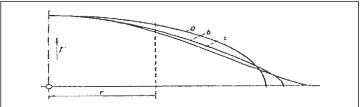
The original theory developed by Prandtl was extended to multiple airfoils by Marx Munk in 1922 (ref. 100) and became what is referred to as “The Biplane Theory”. In his work, Munk introduced the fact that two lifting surfaces will interfere within each others, as one wing will be affected by the downwash of the other one. Therefore, he divided the induced drag equation for two lifting surfaces into four terms: two terms for the individual drag of each surface, and two more for their mutual interference. Finally, he proved that the mutual drag terms are equal. He also applied his theoretical methodology to assess the effect of sweep angle on spanloading in reference (ref. 93) in 1923. A year later, Prandtl published “Induced Drag of Multiplanes” (ref. 92), in which he applied the theory developed by Munk to systems of two and three elliptically loaded lifting surfaces. The resulting solution was a simple, lightweight equation using sigma (σ) factors that allowed designers to quickly estimate the induced drag on any two or three wings aircraft configuration. At this point, it seemed understood and accepted that an elliptical lift distribution could minimize the induced drag of a lifting surface. The downwash of an ideal spanloading could be defined as a Y = C function. However, the design of an aircraft is a compromise between multiple disciplines, and Prandtl noted in his work that the structural weight associated with the elliptical spanloading (see spanload “a” on next figure) was not necessarily the optimum distribution. He proposed in 1932 (ref. 35) a solution to obtain the ideal spanloading of a wing with a constrained root bending moment. His conclusions were that the ideal wing would have a 22% increase in span with an 11% induced drag reduction. As for the ideal spanloading, its shape was more triangular than elliptical (b and c).

Figure 1.3 Prandtl’s ideal spanload for a constrained root bending moment Taken from reference 35 (2006, p. 7)

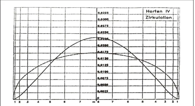
During and after World War II, from 1940 to 1955, the Horten brothers used Prandtl’s latest spanload work to develop their flying wings designs. They introduced concepts such as the induced thrust at tips and the “Mitteleffekt” (ref. 35). They eventually solved for an ideal spanload constrained for root bending moment and stability requirements, which is referred to as the “Bell Shaped” spanload.

Figure 1.4 Horten brother’s “Bell Shaped” spanloading for flying wing Taken from reference 35 (2006, p. 8)

In 1950, Jones published a work (ref. 101) in which he solved for an ideal spanloading with constraints on lift and bending moment. However, his calculation of the root bending moment is less general than Prandtl’s. He concluded that a 15% reduction of induced drag was possible with a 15% increase in span as compared to an elliptically loaded wing of equal lift and bending moment. Just like Prandtl, the resulting spanload is more triangular. Nevertheless, even if the drag reductions predictions differ from Prandtl to Jones, one can notice an obvious similarity in the spanload shapes.

Figure 1.5 Jones’s ideal spanloading with constrained root bending moment Taken from reference 101 (1950, p.14)

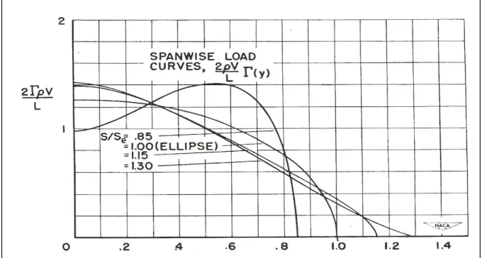
In 1967, Lundry (ref. 34) performed an investigation to solve for the minimum induced drag spanloading while constraining the lift and span of a swept wing to achieve zero pitching moment. This work was, in most point, very similar to the Horten’s work, with the fundamental difference that Lundry was trying to quantify the drag penalty of trimming the aircraft by shaping the spanload. It is however very interesting to see that he obtained the same “bell shaped” distribution that the Horten’s.

Figure 1.6 Lundry’s ideal spanloading Taken from reference 34 (1967, p. 2)

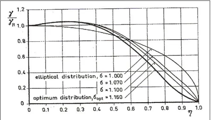
The work done by Prandtl, Horten, Jones and Lundry introduced a new dimension in spanload optimization, as the ideal downwash distribution was now defined as a Y = BX + C function. Several years later, in 1975, Klein and Viswanathan (ref. 65) performed an investigation to solve for the ideal spanload of a wing with constrained structural weight, including bending moments and shear stresses. They concluded that a 7% reduction of induced drag was possible with a 16% increase in span compared with an elliptically loaded wing of equal weight.

Figure 1.7 Klein and Viswanathan’s ideal spanload for constrained wing weight Taken from reference 65 (1975, p. 3)

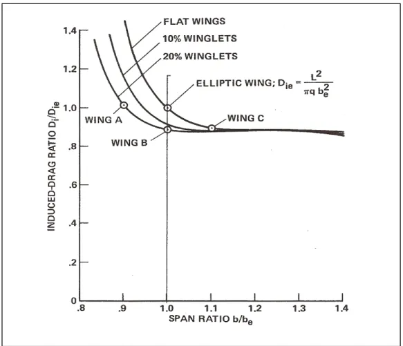
This work defined the ideal downwash distribution as a parabolic function Y = AX2 + BX + C. For the reader who would like to seek more details about the approaches mentioned herein, Jones published a summary in 1979 (ref. 35). Up until this time, most of the research done on spanloading was focused on the assessment of ideal lift distribution over a single planar wing. In 1980, Jones and Lasinski (ref. 103) obtained an analytical solution for the ideal spanload of wings with winglets by constraining the area under the bending moment curve; the same approach used by Prandlt. They observed that for an ideal wing shape,

similar reductions of induced drag can be achieved by either horizontal or vertical tip extensions.

Figure 1.8 Jones and Lasinski’s drag reduction with winglets Taken from reference 103 (1980, p. 21)

At this point, the lift distribution optimization was now assessing non-planar lifting surfaces. However, since the foundation of the solution was still based on Prandtl’s lifting line theory, the induced drag was computed in a planar manner. During the same period of time, Kroo proposed a method in (ref. 26) that allowed to solve for the ideal spanload distribution that minimizes the induced drag of any biplane configuration. His approach was based on Prandtl’s work “Induced Drag of Multiplanes” cited previously. By considering an elliptical lift distribution over the second lifting surface (canard or tail), the minimum drag spanload over the wing can be obtained. He also proposed a general equation very similar to the one

published by Prandtl in 1924, with the simple addition of sigma* (σ*) factors, which can be calculated or extracted from graphics. No structural calculations were included into this work.

Kroo’s method was later extended to three lifting surfaces configurations by Laurendeau in 1990 (ref. 108). The same assumption of elliptical spanloading on the secondary and tertiary surfaces was used. The method allows to solve for the minimum induced drag spanloading over the wing and new sigma* (σ*) factors are determined. Laurendeau’s approach offers an analytical solution for the induced drag of multiple lifting surfaces aircrafts that seems appropriate for actual needs. However, since it is based on the lifting-line theory, the drag calculation is done like if the wing was planar, without consideration for the sweep or dihedral. Even so, recent literature let believe that fairly good accuracy can be expected from it. To mention a few, the following authors have used linear and non-linear lifting-line approaches (NL-LLT) in their work for various applications and managed to obtain satisfactory precision for conceptual design purposes.

Chi (ref. 88) uses numerical lifting-line for icing simulation and compares with CFD. He obtains results that are within 2-5% error. Cheng (ref. 84) applies the same method on forward-swept wings (FSW) and concludes that such wings performances can be properly estimated using simple correlations with aft-swept wings (ASW). Owens (ref. 85) investigates numerical NL-LLT as a tool to be used for aircraft design and obtains good results according to data. In ref (ref. 86), Funk implemented a similar approach into a six degree-of-freedom (6-DOF) model to simulate stall departure of a Cessna. Results compare well to flight data on general aviation aircraft. Ariyur (ref. 87) uses numerical lifting-line to model ground effect and compares with a Gulfstream V. Results are satisfactory and the author suggests ways to improve accuracy.

This concludes the review of the literature for this work. All theoretical bases employed for the development Laurendeau’s method and LLT software are detailed next.

CHAPITRE 2 THEORY

2.1 The Biot-Savart Law and Kutta-Joukowski Principle

Before starting any development on Prandtl’s lifting-line theory, it seems appropriate to quickly introduce the two fundamental principles on which it is based: the Biot-Savart law and the Kutta-Joukowski principle.

The Biot-Savart law is used to calculate the velocity “V” at a given point “P” located at a certain distance “r” from a segment “dl” located on an infinite vortex filament of strength “Γ”. To make an analogy with electromagnetism, the vortex filament would be an electric wire carrying an electrical current “Γ” and the resulting magnetic field at point “P” would represent the velocity induced by this filament. For application to aerodynamic, the Biot-Savart law goes as following:

3 4 dl r V r π ∞ −∞ Γ × =



This fundamental principle applies for any vortex filament. However, the lifting-line theory uses only semi-infinite straight filaments as illustrated on the next figure.

Figure 2.1 Velocity induced at point P by a semi-infinite straight vortex filament V x z y a dl θ r h Γ ∞ P

The application of Biot-Savart law to this simplified system reduces to: 0 2 0 / 2 sin sin 4 4 4 V dl d r h π h θ _{θ θ} π π π ∞ Γ Γ Γ =





Thus, the velocity induced at a given point “P” by a semi-infinite, straight vortex filament at a perpendicular distance “h” from “P” is simply Γ/4πh.

The second fundamental principle used by Prandtl is the Kutta-Joukowski principle. This principle defines lift force “L” as a function of the strength “Γ” of a vortex filament, or circulation.

L=_ρVΓ (2.3)

This result underscores the importance of the concept of circulation, as it links together the strength of a vortex to the generation of lift. Its fundamental meaning is that the lift per unit span is directly proportional to the circulation around the body. Now that the basics are well established, the lifting-line theory can be developed.

2.2 Prandtl’s Lifting Line Theory

Prandtl had understood that the very low pressures over a finite wing would force the air to roll around the tip, pushing the flow over the wing to move inboard, and similarly, forcing the air under the wing to move outward. The resulting difference in spanwise velocity causes the air to roll up into a several streamwise vortices, influencing the lift force along the span.

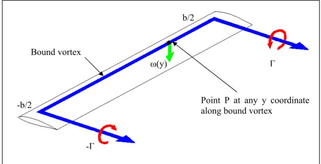
In his lifting-line theory, Prandtl modeled these streamwise vortices using Biot-Savart law as vortex model, and linked vortices from both sides of the plane together with a bound vortex of equal strength; creating what is called a horseshoe vortex. The figure below illustrates a single horseshoe vortex on a finite wing.

Figure 2.3 Single horseshoe vortex over a finite wing

Using Biot-Savart law, the velocity at point P at a given spanwise coordinate “y” on a wing of span “b” induced by the free-trailing vortices can be calculated as following.

(

)

(

)

(

)

This downward velocity “ω(y)” induced at point “P” by the trailing vortices is called downwash, and changes the local effective angle of attack of this particular wing section. The lift force generated at this coordinate is therefore diminished and inclined backward. Thus, the local effective lift of this wing section has a component of force parallel to the undisturbed freestream flow. This drag force is a consequence of generating lift on a finite wing and is called induced drag, or vortex drag.

-Γ -b/2

b/2

Γ

Point P at any y coordinate along bound vortex

Bound vortex

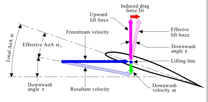
Figure 2.4 Induced flow over a wing section

To determine the spanwise lift distribution and the induced drag of a complete finite wing, Prandtl superposed an infinite number of horseshoe vortices along the lifting line. Each of these vortices has a vanishingly small strength “dΓ” corresponding to an infinitesimally short segment of the lifting line “dy”. Let us single out a segment “dy” located at “y” having a circulation “Γ(y)” and a change of circulation along the segment “dΓ”. Therefore:

d dy

y ∂Γ Γ =

∂ (2.5)

Substituting the latest into (2.2), the downwash variation induced by this segment on any point P located arbitrary at a coordinate y0 along the lifting line is:

(

)

(

)

To compute the total velocity induced at the spanwise coordinate y0 by the entire trailing

vortex sheet, equation (2.6) is integrated from one tip to the other.

Lifting line α Effective AoA Downwash ε angle Freestream velocity velocity Downwash ω α Loc al A oA _e ε Downwash angle Effectve lift force force Di Induced drag lift force Upward Resultant velocity

(

)



Note that the integration boundaries for the tips are not defined as b/2 and –b/2, as they have been replaced to take into account the dihedral angle and winglets. The integration is then performed as a line integral along the wingspan, like if a non-planar wing was unfolded into an equivalent planar surface.

Figure 2.5 Induced velocity at point P by superposition of horseshoe vortices along a lifting line representing a non-planar lifting surface

From (2.7), the local downwash angle ε(y0) can be obtained from trigonometry.

1 0 0 0 ( ) ( ) ( ) tany y y V V ω ω ε ₌ −  _{≈ −}     (2.8)

Where V is the freestream velocity. From figure 2.5, the local induced drag at point P located at coordinate y0 from the center of the wing follows.

0 0 0 ( ) ( )sin( ( )) Di y =L y _ε y (2.9) -b/2 b/2 -s s P

In (2.9), the local lift L(y0) at point P is obtained from the Kutta-Joukowski principle (2.3).

The substitution of this principle into (2.9) reduces to:

0 0 0

( ) ( ) ( )

Di y =_ρω y Γ y (2.10)

By integrating (2.3) and (2.10) over the entire unfolded span, the wing’s total lift force and corresponding induced drag can be obtained.

s ( ) s L _ρV y dy − =





Prandtl extended his research to solve for the circulation distribution that would minimize the induced drag of a finite wing: the elliptical spanloading. However, there is no need to detail this part of his work as it is not used for further development in this report. The demonstration of this solution is frequently detailed in books such as the ones published by Anderson (ref. 110) or Bertin (ref. 111). The only relevant equation for this work concerning the elliptical lift distribution is the following, concluding this section on the lifting-line theory.

Di_Elliptical L2 ₂ qb

π

= (2.13)

2.3 Munk’s Biplane Theorem

Munk used Prandtl’s lifting-line theory and the Biot-Savart law to assess the fundamental principles related to systems of multiple lifting surfaces. The details of his approach are available in (ref. 100). However, for the purpose of this work, it does not seem necessary to go through the whole theoretical process as only the conclusions will be used for further developments.

Using the Biot-Savart law, Munk obtained a solution for the downwash velocity induced on a given wing element by a second wing. The following figure illustrates in a visual manner the influence of the circulation over a wing influencing the downwash velocity on another nearby lifting surface.

Figure 2.6 Mutually induced downwash velocities on two lifting surfaces

Recalling Prandtl’s equation (2.10), the induced drag at a point y, located on wing 2, generated by wing 1 is quantified as following:

12( ) 12( ) ( )2

Di y =_ρω y Γ y (2.14)

He also understood that if the circulation around wing 1 had influence over the second wing, then the circulation around the second wing would also influence the first one.

21( ) 21( ) ( )1

Di y =_ρω y Γ y (2.15)

The integration of these equations, in the same way done by Prandtl from (2.10) to (2.12), allows defining the total drag of the system as a summation of four terms.

Di_system =Di₁+Di₁₂+Di₂₁+Di₂ (2.16) (y2) (y2) (y1) (y1) WING 1 ω21 Γ1 Γ2 ω12 WING 2

A proper assessment of the mutual downwash velocities ω12 and ω21, which are not constant

along the span, is required to obtain a solution. Throughout his developments, Munk stated two fundamental theorems that will be of assistance in what follows.

“Any system, as regard its total induced drag, is equivalent to a simpler system having the same front view, in which the centers of pressure of all the constituent wing surfaces, while maintaining the same lift distribution, are shifted into one and the same plane, at right angles to the direction of flight.” (M. Munk, ref. 100).

“In an unstaggered wing system, the drag D12, induced by wing1 on wing 2, equals

the drag D21 induced by wing 2 on wing 1.” (M. Munk, ref. 100).

From these theorems, equation (2.16) may be simplified.

1 2

system mutual

Di =Di +Di +Di (2.17)

Where Dimutual is the double of the interference drag induced by a single wing to another.

Di_system =Di₁+2Di₁₂+Di₂ =Di₁+2Di₂₁+Di₂ (2.18)

2.4 Prandtl’s Equation for Multiplanes

As mentioned in the previous section, to properly evaluate the total induced drag of a system containing multiple lifting surfaces, it is necessary to have an appropriate calculation of the spanwise downwash velocity profile ωxx(y) of the wings. To assess that, Prandtl (ref. 92)

used a graphic representing the spanwise downwash velocities (here called “z”) induced by a flat plate for several vertical distances (gap “G”), expressed as a fraction of the span (b1).

Figure 2.7 Spanwise downwash velocities ω(y) for various gaps Taken from reference 92 (1965, p. 20)

This flat plate analysis was originally proposed by Munk and the test results were performed by Wr. K. Fohlhausen. To simplify the use these curve, equation (2.14) is adapted using the Kutta-Joukowski principle and the term ρΓ2 is replaced by δL2/V. The interference drag can

be obtained by integrating from tip to tip according to lifting-line theory (2.12).

12 12 2 ( ) ( ) s s y Di L y V ω _δ − = −



Prandtl makes a final adaptation to the ω12(y) term, since both wings 1 and 2 might not have

1 12 2 1 2 ( )y L z y( ) Vb ω π = (2.20)

The z(y) term is directly obtained from the preceding figure, and the drag induced by wing 1 on wing 2 can now be calculated by solving the integration (2.19). This integral was evaluated at the time using planimetry for various span ratios b2/b1 and different values of the gap G/b1 on the assumption the lift distribution over wing 2 is elliptical. The result makes use of an interference factor “σ” which can be obtained graphically.

1 2 12 21 1 2 2 2 2 mutual L L Di Di Di qb b σ π = = = (2.21)

The total induced drag of any biplane configuration can now be obtained by the substitution of (2.21) and (2.13) into (2.17). This relation is known as The Biplane Equation.

2 2 1 1 2 2 2 2 1 1 2 2 2 Biplane L L L L Di qb qb b qb σ π π π = + + (2.22)

The biplane equation was reworked in 1980 by Laitone (ref. 28), who added Oswald efficiency factor “e” to each terms of (2.22). It was later extended to three lifting surfaces configurations by Kendall in 1985 (ref. 27). The resulting induced drag for the system is:

2 2 2 3 2 32 3 1 3 13 1 1 2 12 2 2 2 2 1 1 2 2 3 2 3 1 3 2 2 2 Triplane L L L L L L L L L Di qb qb b qb qb b qb qb b σ σ σ π π π π π π = + + + + + (2.23)

The sigma (σ) factors required to use these equations can be obtained from the following figure where the x axis is the span ratio b/bwing and r is the vertical gap between each lifting

Figure 2.8 Prandtl’s interference factor σ Taken from reference 92 (1965, p. 20)

Of course, using this approach means that we recognize and accept Prandtl’s methodology, which considers elliptical lift distribution over all lifting surfaces, which is not always the case.

In order to be able to compute the induced drag of non-elliptical lift distribution, the following chapter introduces an approach to define analytically any spanload distribution over a wing so that it can be used in the methods defined earlier.

2.5 Technique for General Spanwise Circulation Distribution

The technique for general spanwise circulation distribution consists in representing the circulation by a Fourier sine-series composed on “n” terms. A detailed development of the method is available in Anderson (ref. 110) and Bertin (ref. 111). Figure 2.9 represents the behavior of the circulation distribution as the Fourier series is modified.

Γ 0 π π/2 A1 sin(θ) (3θ) +A3 sin A1 sin(θ) (θ)

A1 sin +A3 sin(3θ)+A5 sin(5θ)

Figure 2.9 Circulation distribution represented by Fourier series

As illustrated on the figure above, adding terms to the series increases the “flexibility” of the curve. If only one term is considered, the distribution is elliptical. By altering the An Fourier coefficients, it is possible, if the series is composed of a sufficient amount of terms, to model about any shape of spanwise circulation distribution over a wing. Only odd terms (1,3,5…) are used to model the spanloading since they assure a symmetrical behavior of the curve from one tip to the other. However, since Fourier series are simpler to use in a polar coordinate system, it is convenient to replace the Cartesian spanwise coordinates (y) by the equivalent polar (θ) coordinate. Consider the transformation:

cos( )

In the latest equation, one must remember that the “s” variable represents the “unfolded” spanwise coordinate as illustrated in figure 2.5. Any circulation distribution over a wing can be defined by the following Fourier series with n = 1, 3, 5 and θ being the spanwise location.

1

( ) 4_θ sV N A_nsin( )n_θ

Γ =



The lift force corresponding to this distribution can be obtained by applying the coordinate system transformation (2.24) to the lift equation (2.11) defined in the lifting-line theory, and by substituting (2.25) into it.

2 2 0 ( ) 4 sin( )sin( ) s n s odd L _ρV y dy _ρV s π A n_{θ θ θ}d − =







The same approach is repeated with (2.12) for the induced drag calculation.

2 2 0 ( ) ( ) 4 sin( ) sin( ) s n n s odd odd Di _ρω y y dy _ρV s π nA n_θ A n d_{θ θ} − =









These two integrals can be solved and reduced to very simple relations.

2 1 4 L= _πqs A (2.28) 2 2 2 1 n odd A L Di n qb A π   =    



Therefore, the lift generated by a given Fourier distribution over a wing can be computed from the A1 coefficient only. As for the induced drag, there is an obvious similarity with

Prandtl’s elliptical spanload equation (2.13), with the only addition of the summation term. The following section details how Fourier distributions can be used into Prandtl’s equation for multiplanes.

2.6 Kroo’s Method

Kroo proposed in 1982 (ref. 26) a method to solve for the minimum induced drag spanload over a wing influenced by a secondary elliptically loaded lifting surface. Summarizing his approach, the Fourier series technique explained in the previous section was used to define the circulation distribution over the primary wing. To describe the downwash velocities ω12

induced by a secondary lifting surface on the wing, an analytical methodology given by von Kármán and Burgers (ref. 112) was applied. The induced drag equation for a biplane (2.22) was then rewritten to accommodate the non-elliptical loading on the wing. By derivation of this newly adapted formulation, the Fourier coefficients An that define the minimum induced drag spanloading were obtained by the derivation δDi / δAn = 0.

Once again, the key in this solution is to properly evaluate the downwash velocities induced by one wing on another. The method proposed by von Kármán and Burgers is a mathematical representation that approaches the velocity fields used by Prandtl on Figure 2.7. To clarify the upcoming developments and the ones that will follow in further sections, the reader may consider indices 1 and 3 to represent the secondary lifting surfaces (canard or stabilizer) as indices 2 refers to the main wing. The local downwash velocity induced on a given segment of the main wing by a secondary lifting surface is defined as following.

12 2 01 1 Re 1 ω ξ ω _ξ     = − _{ } −   (2.30)

In this equation, the local induced downwash velocities ω12 on the wing are expressed as a

ratio of the ω01, which represents the downwash velocity at the root of the secondary lifting

surface. The term ξ is obtained from:

1 1

2y 2h i

b b

where b1 is the span of the secondary lifting surface, h the vertical separation between the

wings and y the spanwise coordinate on the main wing. The term ω01 can be expressed by:

2 01 2 2 L V qb ω π = (2.32)

From these equations, the downwash velocities mutually induced between two lifting surfaces can be obtained. The figure below illustrates these velocities for various vertical gaps between a wing and a secondary lifting surface of span b1 = 0.625 b2, which is exactly

the same figure used by Prandtl (see Figure 2.7), with the only difference that he quantified the gap as a function b1.

Figure 2.10 Induced downwash velocities on surfaces 1 and 2 for various vertical gaps Secondary wing on main wing

No Gap

Gap = b2/2

Recalling (2.17), the total induced drag of the system is the summation of the individual drag of each lifting surface and the mutual drag resulting from their interference. The drag of the main wing and the secondary lifting surface are calculated respectively using (2.29) and (2.13). The mutual drag is twice the drag induced by one wing on the other and is calculated by solving (2.12). 12 12 2 2 2 s ( ) ( ) mutual _s Di Di _{ρ ω} y y dy − = =



The circulation distribution over the wing Γ2(y) is defined by Fourier series in polar

coordinates and the downwash velocity field ω12 is obtained from von Kármán and Burgers

equations. By substituting these terms into the integration, we have:

2 0 1 2 12 2 2 2 01 1 4 sin( ) n mutual odd A L L Di n d qb _π A ω _{θ θ} π ω     =        





The coordinate system transformation (2.24) can be reversed by posing:

cos y y s θ = = − (2.35)

The total drag of the system is therefore defined by:

2 2 1 1 2 1 2 2 2 2 1 1 2 2 2 Biplane L L L L Di qb qb b qb σ σ π π π = + + (2.36) with 2 2 1 n A n A σ =    



2 1 12( ) 1 1 4 _n n odd A b I b A σ π   =    





Therefore, the induced drag of a biplane, for which the circulation distribution over the wing is defined by several Fourier coefficients An, can be obtained. Kroo proposes a method to

solve for the An coefficients that will minimise the induced drag of the system by derivation

of (2.36). 0 n Di A ∂ ₌ ∂ (2.40)

The An coefficients for minimum induced drag can be isolated from the solution of this

derivation.

(

)

The A1 coefficient determines the lift of the wing and is obtained from (2.28). By substitution

of this latest equation into (2.37) and (2.38), the sigma (σ) factors for minimum induced drag are obtained. Equation (2.36) can finally be reduced to:

2 * 2 1 1 2 2 2 2 1 1 2 2 2 BiplaneMin L L L L Di qb qb b qb σ σ π π π = + + (2.42) 12(1) 1 2 4 ( / ) I b b σ π = (2.43) 2 12( ) * 2 3 1 2 16 1 ( / ) N n I b b n σ π = −



The σ factor obtained by Kroo is the same as Prandtl’s interference factor illustrated in figure 2.8. However, its calculation is now completely analytical, which saves us the trouble of having to rely on planimetry! As for the σ* factor, its use in conceptual design allows to quickly assess the minimum induced drag achievable by any biplane configuration. The following figure illustrates the σ (blue curves) and σ* (red curves) interference factors in function of the gap between the wings and the ratio of their span.

Figure 2.11 Prandtl and Kroo interference factors

This concludes the theory behind Kroo’s method. The last theoretical concept required for the future developments of this work is introduced in the following section.

Span Ratios bn/b2 a = 1.0 b = 0.8 c = 0.6 d = 0.4 e = 0.2 a c b d e

2.7 Laurendeau’s Method

Laurendeau proposed in 1990 (ref. 108) an extension to the method developed by Kroo by adding a third lifting surface to the system. This third wing is considered elliptically loaded, which is the same assumption used by Kroo for his secondary lifting surface. By derivation of the induced drag equation for the complete system, the An coefficients defining the

minimum induced drag spanloading of any three lifting surfaces configuration can be solved, and the corresponding σ factors are obtained.

Recalling Prandtl, the total induced drag of a system composed of multiple lifting surfaces will contain one term for the induced drag of each individual wing, and one mutual drag term for each pair of wings. For a three lifting surface configuration, the induced drag equation will therefore be composed of six terms as showed in (2.23).

Di_Triplane =Di₁+Di₂+Di₃+Di₁₂ +Di₃₂+Di₁₃ (2.45)

Once again, indices 2 refer to the main wing, as indices 1 and 3 are used for the canard and stabilizer. In this latest expression, the terms Di1 and Di3 are evaluated using (2.13) since

both surfaces are elliptically loaded. As for the drag of the main wing, it is obtained using (2.29), which is exactly the same thing as using (2.13) multiplied by the σ2 factor described

by (2.37). The mutual drag terms Di12 and Di32 are assessed in the exact same way as in the

previous section. Recall the integration (2.34), the equation for the mutual drag of any secondary surface k interfering with the primary wing is defined as following.

2 2 2 2 2 _{k k} k k L L Di qb b σ π = (2.46)

Where σk2 is obtained from (2.38). The only missing term is the mutual interference drag

between the two secondary surfaces. Relation (2.46) can be reworked to allow the calculation of Di13.

1 3 13 13 1 3 2L L Di qb b σ π = (2.47)

To obtain the σ13 factor, the development of equation (2.38) is applied to elliptically loaded

surfaces only and reduces to;

13 13 1 3 4 ( / ) I b b σ π = (2.48) with 1 1 13 13 01 0 sin(cos ) I ω y d y ω −   =    



Regrouping all six terms, equation (2.45) can be rewritten.

2 2 2 3 2 32 3 1 3 13 1 1 2 12 2 2 2 2 2 1 1 2 2 3 2 3 1 3 2 2 2 Triplane L L L L L L L L L Di qb qb b qb qb b qb qb b σ σ σ σ π π π π π π = + + + + + (2.52)

Following Kroo’s approach, Laurendeau applies derivation (2.40) to obtain the An

coefficients corresponding to the minimum induced drag of the system.

(

)

(

)

This result is then inserted into the calculation of the multiples σ factors. Equation (2.52) is modified to include Kroo’s σ* factors for minimum induced drag.

2 * * 2 * 2 3 2 32 3 3 1 3 13 1 1 1 2 12 2 2 2 2 1 1 2 2 3 2 3 1 3 2 2 2 TriplaneMin L L L L L L L L L Di qb qb b qb qb b qb qb b σ σ σ σ σ π π π π π π = + + + + + (2.54)

In this last relation, the σfactors are Prandtl’s interference factors and are obtained using (2.43). As for the σk* factors, they can be obtained from (2.44) and Laurendeau proposes a

solution for the σ13* factor, expressing the interference between the canard and stabilizer.

12(1) 12 1 2 4 ( / ) I b b σ π = (2.55) 32(1) 32 3 2 4 ( / ) I b b σ π = (2.56) 2 12( ) * 1 2 3 1 2 16 1 ( / ) N n I b b n σ π = −







This concludes the overview of the theory used throughout this work. The following sections of this chapter are meant to verify the robustness of Kroo’s and Laurendeau’s equations.

2.8 Theory Robustness 2.8.1 The “Zero - Gap” Cases

The use of Prandtl’s equations for the analysis of multiple lifting surfaces aircrafts results to a numerical problem: the Biot-Savart law, on which Prandtl’s theory is based-on, has a singularity in the center of a vortex; singularity that occurs at the tip of a lifting surface. In the case of a multiplane with no stagger between lifting surfaces, a mathematical discontinuity occurs at the tip of each lifting surfaces having a smaller span than the main wing. Recalling figure 2.10, a “zero-gap” configuration results in a mutually induced downwash tending to infinity at the tip of the shortest lifting surface. This is due to the fact that a singularity occurs in the calculation of the induced downwash velocity defined by (2.30) : 12 2 01 1 Re 1 ω ξ ω _ξ     = − _{ } −   (2.60)

In this equation, the value of ζ equals zero for zero-gap cases, which results in an infinite downwash velocity and numerical error. Therefore, in the implementation of the “LLT” program, a special case was added for zero-gap conditions, replacing ζ = 0 by ζ = 10-7. This small induced imperfection has shown not to provoke any computation errors up-to seven digits after zero and insures robustness of the computational process.

The singularity in Biot-Savart equation also induces a computational difficulty in the calculation of the σ and σ* factors for near-zero gap conditions. The exact solution of integration (2.39) has been solved into the following interference factors:

σ = b1/b2 (2.61)

In order to attain such results numerically and assuming a linear discretisation of the span, one should consider using 1000 wing section cuts semi-spanwise to solve the (2.39) integration numerically and obtain proper computation of the σ and σ* factors to within 10-7.

2.8.2 Interchangeability Front - Rear

This validation test is made to make sure that Kroo’s and Laurendeau’s equations are correct and that no typological errors have slipped through correction. As a first experiment, the interchangeability of wings 1 and 2 in the equations is investigated. Since the induced drag calculation is done independently of the depth of each lifting surface, the drag result should not vary when wing’s identification number is changed in the equation.

=

?

1

2

3

3

2 1

3

2

1

?

=

Figure 2.12 Validation of Front-to-Rear Interchangeability in the Equations

Subsequent to a mathematical verification, it was determined that the equations are robust and consistent in term of front-to-rear interchangeability as long as the main wing has a larger span than the two other lifting surfaces. Consequently, one should clearly predetermine the numerical indices relating to each lifting surfaces. For the remaining part of this work, the indices “2” will represent the main wing, having the largest span. The wingspan of the other lifting surfaces is therefore expressed as a fraction of the main span. In no case wings number 1 and 3 can have a larger wingspan than wing number 2, since the fundamental theory concerning the mutual downwash equations will no longer be functioning.

2.8.3 Interchangeability Top - Bottom

In the same train of thought than for the previous section, the top-to-bottom interchangeability of the equations was investigated. Once again, induced drag results should not vary with the identification of the lifting surfaces since the aircraft configuration is the same.

?

=

=

?

Figure 2.13 Validation of Top-to-Bottom Interchangeability in the Equations

An analytical verification shows that the equations are robust and consistent as long as the value of the gaps between various lifting surfaces are positive and expressed as a fraction of the main wingspan. Therefore, if one supposes an aircraft having a reference wingspan of 100 feet, a tailspan of 30 feet and a stagger height of 20 feet, the aircraft definition for use in the equations goes as following:

2 12 1 2 12 12 2 1 / 0.3 2 / 0.4 b b b b h h b = = = = =

CHAPITRE 3 IMPLEMENTATION 3.1 Software Description

In order to asses the induced drag of multiple lifting surfaces aircraft configurations, the various theories summarized in the previous chapter were implemented into a program called LLT. The software was written in Matlab and can compute the induced drag of any one, two or three lifting surfaces configuration in less than 0.10 seconds on an average dual-core PC. The necessary inputs and resulting outputs are described below.

LLT inputs:

• An input file, in text format, containing various geometry and lift coefficients for the canard, stabilizer and wing;

• If specified by the user, a spanload file, in text format, detailing the discretisation of the wing. It contains the height and spanwise coordinates for every wing element and the related adimensionalized normal force coefficient.

LLT Internal Operations:

• Calculation of the An coefficients corresponding to the input spanload distribution; • Induced drag calculation for the main wing with winglets;

• Correction of the main wing’s induced drag to include the fuselage effect; • Calculation of the total induced drag of the aircraft.

LLT Outputs:

• Exports an induced drag report in text format; • Displays a figure of the various lift distributions;

breal 3.2 Main Wing Induced Drag Calculation

As a first step to the development of LLT, the induced drag of a single wing-winglet-body was implemented. The dihedral and spanload distribution are defined by the coordinates in the spanload sheet; coordinates that are expressed in the non-planar “η” coordinate system. Let us pose the following axis systems, which will be used throughout the implementation.

Γ Y or P(y,z) y = 0 y = fus y (P) y = b y = θ Dihed(P) Z or θ = π/2 _θ (P) θ = π θ (P) θ = π θ = π/2 θ y = s y = b y (P) = bod y = 0 P(y) Y or Γ η η η η η s η η s s η η s s s s θs η s s Coordinate System S Coordinate System η

Figure 3.1 Coordinate systems

_ ( ) Cn c P c η× _ Cl c c η× _ ( ) s Cn c P c × _ ( ) s Cn ideal c c ×

According to the lifting line theory, the induced drag of a circulation distribution given by a spanload sheet, without considering the fuselage, can be calculated from :

2 2 / 2 ( ) ( ) 8 sin( ) sin( ) s s s n s n s s s Di y y ds V s π nA n A n d π ρω ρ θ θ θ − =









To solve this, the normal force coefficients Cn c c_y⋅ /_ given for various span locations by the spanload sheet have to be converted into the “s” planar coordinate system. The length “ds” of a spanwise element “I” in the “s” coordinate system can be defined by:

( ) (

) (

)

( )

₍

₎

and ( )δ i being the dihedral of this wing element.

Once the spanload sheet data’s have been converted to a planar coordinate system, the corresponding An Fourier coefficients can be obtained by curve-fitting a Fourier series over

the data. Section 3.2.3 proposes an approach to curve-fit a spanload distribution over input data. However, before this can be done, some adjustments need to be made on the input spanload data concerning the fuselage and the wing tip. As it can be observed on figure 3.2, the data obtained from a spanload sheet is incomplete over the fuselage and tip regions.

s s s s Γ Y or y = 0 y = s θ

Figure 3.2 Spanload definition by imported and created data points

These missing data points are due to the fact that the spanload sheets are generated from several cut planes over the wing on a CFD solution (red points). Therefore, the extrapolated tip loads and exact tip coordinate “s” are unknown, and some realistic data points (green points) need to be added over the fuselage and the tip regions before proceeding to curve-fitting the Fourier series.

3.2.1 Adding Fuselage Data Points The missing data over the fuselage was created by using a 2nd order polynomial following an approach developped by Bombardier Aerospace. Figure 3.3 gives a visual examble of the created fuselage data points using this methodology. The equation 3.4 defines these points.

Figure 3.3 Fuselage data completion Missing Data Input Spanload Coïncidence s s Y orθ P1(y1, z1) P2(y2, z2 ) Γ