CAHIER 22-2001
THE INFLATION BIAS WHEN THE CENTRAL BANK TARGETS THE NATURAL RATE OF UNEMPLOYMENT
CAHIER 22-2001
THE INFLATION BIAS WHEN THE CENTRAL BANK TARGETS THE NATURAL RATE OF UNEMPLOYMENT
Francisco J. RUGE-MURCIA1
1
Centre de recherche et développement en économique (C.R.D.E.) and Département de sciences économiques, Université de Montréal
October 2001
_______________________
This project was started while the author was visiting research fellow at the Bank of Spain in the spring of 2000. The author wishes to thank two anonymous referees for their comments and the Bank of Spain for its hospitality. Financial support from the Social Sciences and Humanities Research Council and the Fonds pour la formation de chercheurs et l'aide à la recherche is gratefully acknowledged.
RÉSUMÉ
Cet article étudie la proposition qu'un biais inflationniste puisse survenir dans une situation où un banquier central ayant des préférences asymétriques cible le taux de chômage naturel. Les préférences sont asymétriques dans le sens que les écarts positifs du chômage par rapport au taux naturel sont pondérés plus (ou moins) sévèrement que les écarts négatifs dans la fonction de perte du banquier central. Le biais est proportionnel à la variance conditionnelle du chômage. Les prédictions du modèle sont évaluées en utilisant des données des pays du G7. Les estimations économétriques soutiennent la prédiction que la variance conditionnelle du chômage et le taux d'inflation sont reliés positivement.
Mots clés : biais inflationniste, préférences asymétriques
ABSTRACT
This paper studies the proposition that an inflation bias can arise in a setup where a central banker with asymmetric preferences targets the natural unemployment rate. Preferences are asymmetric in the sense that positive unemployment deviations from the natural rate are weighted more (or less) severely than negative deviations in the central banker's loss function. The bias is proportional to the conditional variance of unemployment. The time-series predictions of the model are evaluated using data from G7 countries. Econometric estimates support the prediction that the conditional variance of unemployment and the rate of inflation are positively related.
1
Introduction
This paper studies the proposition that an in°ation bias can arise in a setup where a central banker with asymmetric unemployment preferences targets the natural rate. Preferences are asymmetric in the sense that positive unemployment deviations from the natural rate are weighted more (or less) severely than negative deviations in the central banker's loss function. Since the bias is proportional to the conditional variance of the rate of unemployment, the model generates testable cross-section and time-series implications. In a cross section, countries where unemployment is more variable or that are subject to more volatile supply shocks, should have a larger average rate of price in°ation. Preliminary evidence supporting this hypothesis is provided by Gerlach (1999). In a time-series, periods of more volatile unemployment should be associated with a higher in°ation rate. This prediction is formally examined here using data from G7 countries. Maximum Likelihood (ML) estimates support the hypothesis of asymmetric preferences for the United States and France, but not for Canada, Italy, or the United Kingdom.
Previous literature usually assumes that the central banker targets a rate of unemploy-ment strictly below the natural rate. Among others, Persson and Tabellini (2000) note that this assumption is crucial in generating an in°ation bias in the linear-quadratic frame-work of Kydland and Prescott (1977) and Barro and Gordon (1983). The view that the central banker targets a below-natural unemployment rate has been recently challenged on both theoretical and operational grounds. For example, McCallum (1995, 1997) argues that since, in equilibrium, unemployment equals the natural rate but in°ation is larger than optimal, the central banker would eventually understand that the unemployment target is unobtainable and revise its goal. King (1996) and Blinder (1998) suggests on the basis of institutional evidence, that the monetary authority actually targets the expected natural rate of unemployment.
The observation that an in°ation bias can arise even if the central banker targets the natural unemployment rate was ¯rst due to Cukierman (2000). Cukierman outlines two conditions (both of which are satis¯ed here) that are required to deliver the result: (i) uncertainty about next period's realizations of in°ation and unemployment and (ii) asym-metric unemployment preferences. Using a speci¯cation of the loss function where the central banker cares about unemployment only when it is above the natural rate, he ¯nds an in°ation bias that is proportional to the probability of a recession. This paper employs a preference speci¯cation that nests the usual quadratic loss function as a special case, ¯nds an in°ation (or a de°ation) bias that is proportional to the conditional variance of unemploy-ment, constructs an econometric framework to examine the model predictions, and provides empirical evidence that the assumption of asymmetric preferences is plausible for some coun-tries in the sample. Finally, this project complements research by Clarida, Gal¶i, and Gertler (1999) who show that even when the unemployment target corresponds to the natural rate, there are gains from enhancing the central banker's credibility.
The paper is organized as follows: section 2 describes the economy and central banker's preferences, ¯nds the subgame-perfect Nash equilibrium, derives conditions for the existence and uniqueness of the equilibrium, and examines the properties of the in°ation bias; section 3 reports empirical estimates; and section 4 concludes.
2
The Model
2.1
The Economic Environment
Following the literature, in°ation and unemployment are related by an expectations-augmented Phillips curve:
ut = unt ¡ ¸(¼t ¡ ¼te) + ´t; ¸ > 0; (1)
where ut; unt; and ¼t are (respectively) the rates of unemployment, natural unemployment
and in°ation; ¼e
t is the public's forecast of in°ation at time t constructed at time t¡ 1; and
´t is an aggregate supply disturbance. The public constructs its forecasts rationally:
¼e
t = Et¡1¼t; (2)
where Et¡1 is the expectation conditional on all information available at time t¡ 1: The public's information set at time t¡ 1 is denoted by It¡1 and includes the model parameters
and observations of the variables up to and including period t¡ 1: The natural rate of unemployment evolves over time according to
¢unt = Ã + µ1¢unt¡1+¢ ¢ ¢ + µq¢unt¡q+ ³t; (3)
where ³t denotes the unpredictable component of the natural rate and all roots of the
polyno-mial 1¡
q
P
i=1
µiLiare assumed to lay outside the unit circle. This autoregressive model for the
natural rate represents the idea that changes in technology, labor force demographics, and minimum wage rates (among others) can a®ect the labor market and generate movements in the natural rate. For example, Shimer (1998) argues that in the absence of the baby boom, the US rate of unemployment would have neither increased in the 1960's and 1970's, nor fallen afterwards.
The central banker a®ects the rate of in°ation by means of a policy instrument. We can interpret this instrument as a monetary aggregate or a short-term interest rate. The instrument is imperfect in the sense that in a stochastic world, it cannot determine in°ation completely:
¼t = it + ²t; (4)
where it is the policy instrument and ²t is a control error that represents imperfections
in the conduct of monetary policy. Since it is chosen at time t¡ 1; it 2 It¡1: This
simple speci¯cation relaxes the assumption that the monetary authority chooses directly the rate of in°ation after observing (before the public does) the random shocks. Instead, the central banker here has no informational advantage over the public since neither of them observe at time t¡ 1 the realization of the disturbances at time t: As noted by Cukierman (2000), the central banker's uncertainty regarding next period's realizations of in°ation and unemployment is crucial in generating an in°ation bias when preferences are asymmetric.
Finally, the structural disturbances of the model (´t; ³t; and ²t) are serially uncorrelated,
jointly normally distributed with zero mean, and possibly conditionally heteroskedastic. The assumption of normality is essential to obtain a closed-form analytical solution. The assumption of conditional heteroskedasticity allows changes over time in the volatility of
the structural shocks. For example, the net change in nominal oil prices, that could be assimilated to a supply shock, appears to have been more variable in the 1970's than in the 1960's or the 1980's [see Hamilton (1996, ¯gure 2)].
2.2
The Central Banker
The central banker's preferences over in°ation and unemployment are represented by the loss function:
L(¼t; ut) = (1=2)(¼t¡ ¼t¤)2+ (Á=°2)(exp(°(ut¡ u¤t))¡ °(ut¡ u¤t)¡ 1); (5)
where ¼¤
t and u¤t denote the targeted rates of in°ation and unemployment, respectively; Á is
a positive coe±cient; and ° is a nonzero real number. The targeted unemployment rate is the expected natural rate of unemployment:
u¤t = Et¡1unt: (6)
The possibly nonzero rate of in°ation ¼¤
t can be interpreted as the one implied by Friedman's
rule or as the one associated with the optimal in°ation tax. It is assumed that ¼¤
t is stable
enough to be well approximated by a constant term (denoted by ¼¤ below). Section 4
discusses the implications of this assumption.
In contrast to most of the preceding literature where both components of the central banker's loss function are quadratic, the unemployment component in (5) is described by the linex function g(x) = [exp(®x)¡ ®x ¡ 1]=®2 [Varian (1974)]. To my knowledge, the ¯rst
paper to employ this loss function in monetary policy games was Nobay and Peel (1998). In order to develop some intuition, the linex function is plotted in ¯gure 1 for the special case where ° > 0: For unemployment rates above u¤
t, the exponential term eventually dominates
and the loss associated with a positive deviation rises exponentially. For unemployment rates below u¤
t, it is the linear term that becomes progressively more important as unemployment
decreases and, consequently, the loss rises linearly. This asymmetry can be seen in ¯gure 1 by considering, as an example, the loss associated with a §1 unemployment deviation from u¤
t. Even though their magnitudes are the same, the ¡1 deviation delivers a smaller loss
than the +1 deviation. Thus, positive unemployment deviations are weighted more severely than negative ones in the central banker's loss function. The converse is true when ° < 0:
The linex function is attractive for several reasons. First, it is analytically tractable and yields a closed-form solution when shocks are normally distributed. Second, it generates testable empirical predictions (see below). Finally, it nests the usual quadratic loss function as a special case when the preference parameter ° tends to zero.1 This result suggests that
the hypothesis of quadratic preferences over unemployment could be tested empirically by evaluating whether ° is signi¯cantly di®erent from zero. In principle, one could extend (5)
1Formally, Lim °! 0 exp(°x)¡ °x ¡ 1 °2 = Lim °! 0 xexp(°x)¡ x 2° = Lim °! 0 x2exp(°x) 2 = x2 2:
to allow asymmetries regarding the in°ation rate. This possibility is discussed in section 3, where it is argued that the basic predictions of the model are robust to this extension.
The asymmetric loss function means to represent the idea that policy makers have dif-ferent attitudes vis a vis expansions and recessions. In general, both positive and negative deviations from the natural rate are deemed costly, but under (5), the sign of the devia-tion is important for the central banker. In the plausible case where ° > 0, expansions are preferred to recessions. In the empirical literature, Dolado et al. (2000) and Gerlach (2000) ¯nd that the US Federal Reserve reacts more strongly, in terms of changes to the Federal Funds rate, to negative than positive output gaps. Cukierman (2000) considers an asymmetric loss function where the loss is quadratic when unemployment is above the natural rate and zero when unemployment is below. Cukierman's speci¯cation is appealing because it seems likely that, given in°ation, unemployment rates below the natural yield negligible costs (and possibly bene¯ts) to the monetary authority. In contrast, the linex and quadratic loss functions assume a strictly positive cost when unemployment is below the natural rate. As noted by Cukierman (p. 9), the ¯nding of an in°ation bias when the unemployment target is the natural rate depends on the assumption that the central banker is more concerned about too much that too little unemployment. His ¯nding and the one of this paper suggest that this result is robust to the precise functional form of the central banker's loss function, provided this asymmetry is preserved.
2.3
Nash Equilibrium
The central banker's problem is to choose the sequence of instruments that minimizes the present discounted value of her loss function:
M in Et¡1P1
s=0
¯sL (¼
t+s; ut+s) ;
fit+sg1s=0
where ¯ 2 (0; 1) is the discount rate and the public's in°ation forecasts are taken as given. Since the natural unemployment rate is assumed to be determined by factors beyond the scope of monetary policy, the instrument does not a®ect the path of un
t and the central
banker's objective function can be decomposed into a sequence of one-period problems. This decomposition simpli¯es the solution of the model and, as it will be shown below, delivers a unique subgame-perfect Nash equilibrium. The ¯rst-order condition is
Et¡1¼t ¡ ¼¤¡ (¸Á=°)(exp(¡¸°(Et¡1¼t¡ ¼te) + °2¾u;t2 =2))¡ 1) = 0; (7)
where ¾2
u;t represents the conditional variance of unemployment. Since the linex loss function
is globally convex, the second-order su±cient condition for a minimum is satis¯ed. In writing (7), I have used the fact that when shocks are normal, the distribution of unemployment conditional on It¡1 is normal. Hence, the distribution of exp(°(ut¡ Et¡1unt)) is log normal
with conditional mean exp(¡¸°(Et¡1¼t¡ ¼te) + °2¾u;t2 =2)):2
Equation (7) de¯nes implicitly the central banker's reaction (or best move) for any given in°ation forecast by the public:3
h(Et¡1¼t; ¼te)
= Et¡1¼t¡ ¼¤¡ (¸Á=°)(exp(¡¸°(Et¡1¼t¡ ¼te) + °2¾2u;t=2))¡ 1) = 0
(8) Using the implicit function theorem, it is possible to show that 0 < @Et¡1¼t=@¼te < 1 for all
°; and that @2E
t¡1¼t=@(¼te)2 is larger than zero for ° > 0; equal to zero for ° ! 0, and less
than zero for ° < 0: In other words, the central banker's reaction function is monotonically increasing in ¼e
t but can be convex, linear, or concave depending on the sign of °:
In order to develop some intuition, Figure 2 plots the central banker's reaction function for two di®erent values of the preference parameter °: The ¯gure also includes the reaction functions of the public and of a central banker with quadratic preferences. The former is summarized by the rational expectations relation (2). The latter is obtained from (8) by taking the limit ° ! 0 and solving explicitly. The graphs are constructed assuming an optimal rate of in°ation ¼¤ = 0: Treating all parameters as ¯xed, the central banker's
reaction is computed by solving numerically the implicit function (8) for di®erent values of ¼te. The Nash equilibrium is the point where (8) and (2) intersect. In all cases the central
banker's reaction is an increasing function of the public's in°ation forecast. However, her willingness to accommodate agents' expectations varies with the preference parameter °: For the quadratic central banker, the Nash equilibrium corresponds to ¼ = 0; that is the optimal in°ation rate. Hence, the in°ation bias is zero. On the other hand, for ° > 0; (° < 0), an in°ation (de°ation) bias can arise, even if the unemployment target is the natural rate.
Conditions for the existence and uniqueness of the Nash equilibrium are given in the following proposition:
Proposition 1. Provided ° 6= 0; there exists a unique ¼e
t = Et¡1¼t; such that h(Et¡1¼t; ¼et) =
0:
Proof. To prove existence, construct
¼te= Et¡1¼t = ¼¤ + (¸Á=°)(exp(°2¾u;t2 =2)¡ 1): (9)
Plugging (9) into (8) and using ¼e
t = Et¡1¼t delivers h(Et¡1¼t; ¼te) = 0. To show uniqueness,
assume there exists a second in°ation forecast, say ^¼e
t = ¼¤+ (¸Á=°)(exp(°2¾u;t2 =2)¡ 1) +
x; that also lies on the 45± line on the plane (¼e
t; Et¡1¼t) and satis¯es h(Et¡1¼t; ¼et) = 0:
Replacing ^¼e
t in (8), makes clear that the only way h(Et¡1¼t; ¼te) = 0 is if x = 0:{
2.4
The In°ation Bias
The in°ation bias is the systematic di®erence between equilibrium and optimal in°ation. When a central banker with asymmetric preferences targets the natural rate, the bias is:
(¸Á=°)(exp(°2¾u;t2 =2)¡ 1): (10)
3Strictly speaking, the reaction function relates the policy instrument, i
t, to ¼et;both of which are
deter-mined at time t¡ 1. However, in what follows it will be convenient to work with Et¡1¼t rather than it:
For the special case where preferences are quadratic, the bias can be computed by taking Lim (¸Á=°)(exp(°2¾2
u;t=2)¡ 1) = 0:
° ! 0
Since the in°ation bias is zero, monetary policy is not temporally inconsistent under discretion.4
Hence, the theory cannot explain suboptimally high rates of in°ation as the result of the lack of a commitment technology.
Clearly, the ¯nding that the in°ation bias is zero when the central banker targets the natural rate is not robust to relaxing the assumption of quadratic preferences. In the more general case where the central banker's preferences are asymmetric, the in°ation bias is di®erent from zero. This result follows from the observation that ¸Á(exp(°2¾u;t2 =2)¡ 1) is always positive and ° 6= 0, by assumption. The sign of the bias depends on whether ° 7 0: In the case where ° < 0, there is a de°ation bias. More plausibly, in the case where ° > 0; there is an in°ation bias. Recall that ° > 0 means that the central banker attaches a larger loss to positive than negative unemployment deviations from the natural rate.
The bias is proportional to the conditional variance of unemployment. To understand why, recall that when the loss function is quadratic, certainty equivalence holds. The solution of the model is the same regardless of whether there is uncertainty or not, and only the ¯rst (conditional) moment of unemployment explains the rate of in°ation. On the other hand, with asymmetric unemployment preferences, the marginal bene¯t of surprise in°ation is not linear in unemployment, but convex (when ° > 0) or concave (when ° < 0). When ° > 0, an increase in uncertainty raises the expected marginal bene¯t of surprise in°ation.5
This paper relaxes the usual linear-quadratic framework in a particular dimension. That is, it relaxes the assumption of a quadratic objective function but preserves the linear con-straint (the expectations-augmented Phillips curve). Alternatively, one could consider a model where the objective function is quadratic but the supply function is nonlinear. This is the strategy followed by Nobay and Peel (2000). These authors show analytically that the nonlinearity of the supply schedule yields ambiguous implications for the in°ation bias. Nonetheless, there exist parameter values for which a nonlinear Phillips curve could produce an in°ation bias.
For given values of Á and ¸, and ° > 0; the model predicts a positive relation between in°ation and the conditional variance of unemployment. Consider ¯rst the special case where the conditional variance of unemployment is constant. That is, ¾2
u;t = ¾u2 for all t:
Then, the in°ation bias is also (a positive) constant. Because the bias cannot be identi¯ed separately from ¼¤, it is not possible to test the positive relation between ¾2
u and ¼t in the
time series dimension. However, this hypothesis could be examined using cross section data on ¾2
u and average in°ation. Since the unemployment disturbance has the supply shock as 4This result is immediate if one considers the case k = 1 in equation (9) in Barro and Gordon (1983, p.
597), where k is the fraction of the natural rate that is targeted by the central banker.
5There exists a comparable result in the consumption literature. When one relaxes the assumption
of quadratic utility and labor income risk in nondiversi¯able, uncertainty increases the expected marginal utility of future consumption. To satisfy the Euler condition, agents decrease current consumption compared to future consumption and increase savings. Individuals in occupations with more variable income (e.g, farmers) would have above-average savings rates [see Skinner (1988)].
one its components, the model also predicts a positive association between the variance of supply shocks and the rate of in°ation. Evidence supporting this implication is provided by Gerlach (1999) using a cross section of industrial economies.
Consider now the case where the conditional variance of unemployment changes over time. Then, the model predicts that periods of more volatile unemployment should be associated with higher rates of price in°ation. This hypothesis is examined below using time series data from G7 countries.
3
Empirical Analysis
The empirical analysis of the game-theoretical developed above is nontrivial for several rea-sons. First, the natural rate of unemployment is not directly observable. Hence, in order to estimate the model using data on in°ation and unemployment alone, it is necessary to construct a reduced-form version of the model. Second, the conditional variance of the rate of unemployment is not directly observable either. It is possible to construct an estimate of ¾2
u;t on the basis of a fully parametric model like the ARCH or GARCH speci¯cations of
Engle (1982) and Bollerslev (1986). However since ¾2
u;t is then a generated regressor, one
must consider its e®ect on the e±ciency and consistency of the estimates. Finally, it is not possible to recover all structural parameters of the model from the reduced-form estimates. In particular, the preference parameter ° is not identi¯ed. However, we will see below that the sign of the reduced-form coe±cient on ¾2u;t is informative about the sign of °.
The working paper version of this article [Ruge-Murcia (2000)] shows that when the natural rate of unemployment follows the AR(q) process in (3) and the structural shocks are mutually uncorrelated at all leads and lags, the ¯rst-di®erence of unemployment can be written in reduced-form as an unrestricted ARMA(q; q + 1) process. Regarding the in°ation rate, one can use equations (9) and (4) to write
¼t = ¼¤ + (¸Á=°)(exp(°2¾2u;t=2)¡ 1) + ²t: (11)
Notice, however, that it is not possible to identify separately the parameters ¼¤; ¸; Á and
°: To see this, rewrite the above equation as ¼t = (¼¤¡ ¸Á=°) + (¸Á=°) exp(°2¾2u;t=2) + ²t:
An estimate of the intercept term would only deliver the linear combination ¼¤¡ ¸Á=°, and
the time-series variation of ¾2
u;t alone would not identify ¸; Á and °: A transformation of
the model that confronts directly the lack of identi¯cation involves the linearization of the exponential term in (11) by means of a ¯rst-order Taylor series expansion. Then, in°ation can be written in reduced-form as:
¼t = a + b¾u;t2 + ²t; (12)
where a is a constant intercept and b = ¸Á°: Although an estimate of b cannot reveal the values of ¸; Á; and °, its sign is informative regarding the asymmetry in the central banker's preferences. Since ¸; Á > 0, a positive estimate of b implies ° > 0 and would be consistent with the idea that the central banker weights more heavily positive than negative
unemployment deviations from the natural rate.6
The data set consists of quarterly seasonally adjusted observations of in°ation and un-employment for Canada, France, Italy, Japan, United Kingdom, and the United States.7
The in°ation rate is measured by the percentage change (on an annual basis) in the GDP de°ator. The unemployment rate is measured by the average rate of civilian unemployment in the three months of the quarter. The raw quarterly GDP de°ator and the monthly unem-ployment rate were taken from OEDC Main Economic Indicators. The sample period was determined by the ¯rst and latest available observation of both variables in the data base. That is, 1961:1 to 1999:2 for Canada, 1970:1 to 1999:2 for France and Italy, and 1960:1 to 1999:2 for Japan, the United Kingdom and the United States.
Prior to the estimation of the model, econometric tests were employed to examine the time-series properties of the rate of unemployment. Table 1 (panel A) reports the results of Augmented Dickey-Fuller (ADF) and Phillips-Perron (PP) unit-root tests. In all cases, the null hypothesis of a unit root in unemployment cannot be rejected at the 5% level, though the ADF test would reject the hypothesis for unemployment at the 10% level for the United States. Similar results are reported, for example, by Broadbent and Barro (1997) and Ireland (1999) and underpin the modeling of unemployment as an I(1) variable.8
The model with asymmetric preferences predicts a relation between the conditional vari-ance of unemployment and the in°ation rate. It is possible to examine this association in a time series dimension only if unemployment is conditionally heteroskedastic (that is, if ¾2
u;t changes over time). Otherwise, if ¾u;t2 is constant, its coe±cient b is not identi¯ed.
Hence, before proceeding further, it is important to test whether the conditional variance of unemployment is indeed time-varying. Table 1 (panel B) reports the results of Lagrange Multiplier (LM) tests for neglected ARCH. For Canada, the United Kingdom and the United States, the hypothesis of no conditional heteroskedasticity can be rejected at the 1% signi¯-cance level. Similarly, for France, the hypothesis can be rejected at the 10% or 5% levels depending on the number of lags used to compute the statistic. Results for Italy are more ambiguous in that the hypothesis can be rejected at the 10% when two lags are included in the regression but it cannot be rejected in the remaining cases. However, since the p-values are only 0:13; 0:11; and 0:16 when using 1; 3, and 4 lags, respectively, these conclusions ap-pear to be marginal. Finally, for Japan the hypothesis cannot be rejected regardless of the number of lags in the test regression. In summary, test results indicate that the conditional variance of unemployment changes over time in Canada, France, the United Kingdom, and
6When preferences are asymmetric on both in°ation and unemployment, the model solution di®ers from
(11) in the intercept term and the functional form relating ¼tand ¾2u;t: However, since the linearized version
of the model is the same, it would appear that this generalization does not alter fundamentally the model predictions. In principle, one could consider additional regressors (e.g., lagged in°ation) in (12). However, since the model predicts that in°ation depends primarily on the conditional variance of unemployment, I have abstained from including extra regressors and adopted the reduced-form speci¯cation that is closest to the theoretical model.
7I also considered including Germany in the sample. Unfortunately, its series are incomplete or
unavail-able in the data base and reuni¯cation makes hard to compare data before and after 1990.
8Since unit-root tests have low power against persistent, but stationary, speci¯cations, I also estimated
the model under the assumption that unemployment is stationary in levels. Results were very similar to the ones reported and are available from the author upon request.
the United States. There is milder (no) evidence of conditional heteroskedasticity in the case of Italy (Japan). In light of these results, the time series analysis that follows is carried out using data for Canada, France, Italy, the United Kingdom, and the United States.
The model is estimated by the numerical maximization of the joint log likelihood function of in°ation and unemployment.9 The asymptotic variance-covariance matrix is estimated
by the inverse of the Hessian of the log likelihood function at the maximum. Since any stationary ARMA process can be approximated arbitrarily well by a ¯nite autoregression, and the estimation of ARMA processes is frequently complicated by common factors, ¢ut
is estimated in autoregressive form.10 The lag length of the AR representation was
deter-mined using a sequence of Likelihood Ratio (LR) tests. The conditional variance of the rate of unemployment is parameterized using a GARCH(1,1) model. An advantage of this parameterization is that it can capture the persistence of the conditional variance in a more parsimonious manner than higher-order ARCH processes. Recall that the Barro-Gordon model predicts a linear relationship between in°ation and current unemployment. In con-trast, under a GARCH speci¯cation for ¾2
u;t; this model predicts a nonlinear relationship
between in°ation and lagged unemployment.
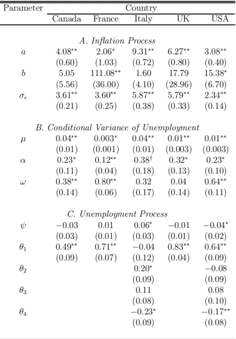
ML estimates of the processes of in°ation, unemployment, and the conditional variance of unemployment are reported in table 2. The coe±cient of the conditional variance of unemployment is positive in all cases and, for France and the United States, it is statistically signi¯cant. For these two countries the null hypothesis b = 0 can be rejected at the 1% and 5% signi¯cance levels, respectively. Recall that because b = ¸Á°, the value of ^b is uninformative about the magnitude of the parameter that measures the asymmetry in the central banker's preferences, °. However, since ¸; Á > 0; a positive ^b implies ° > 0: Hence, positive deviations from the natural unemployment rate appear to be weighted more heavily than negative ones in the central banker's loss function. This result could explain the empirical ¯nding by Dolado et al. (2000) and Gerlach (2000) whereby the US Federal Reserve reacts more strongly to negative than positive output gaps.
For Canada, Italy, and the United Kingdom, ^b is positive but its standard error is large enough that one would not reject the hypothesis that the slope coe±cient equals zero. This result is compatible with the standard model where the loss function is quadratic and the conditional variance of unemployment has no explanatory power over the rate of in°ation. Hence, for these countries, departures from quadratic unemployment preferences appear to be small or perhaps not of the functional form explored here.
The countries for which b is statistically di®erent from zero, are also the countries for which the conditional variance of unemployment is the most persistent. Figure 3 plots the impulse response associated with a 1 standard-deviation innovation to ¾2
u;t. Notice that
for Canada, Italy, and the United Kingdom, the e®ect of the innovation on the conditional variance is not very persistent. After 2 quarters, the e®ect is half or less than half the
9An alternative estimation strategy involves computing ¾2
u;tusing the unemployment series and then
run-ning an OLS regression of ¼ton ¾2u;t: This strategy yields less e±cient estimates than Maximum Likelihood
because it does not impose the cross-equation restrictions of the model and does not exploit the contem-poraneous correlation of the reduced form disturbances. Results using OLS yield the same conclusions as those based on ML and are available from the author upon request.
10Results using a low-order ARMA process yielded virtually the same results as reported below. These
initial shock. On the other hand, for France and the United States, innovations to ¾2 u;t
are much more persistent. After 8 quarters (2 years) the e®ect is still 0:55 and 0:37 of the initial shock, respectively. This result provides another interpretation for the ¯nding that b is not statistically signi¯cant in the case of Canada, Italy, and the United Kingdom: the time-variation in the conditional variance of unemployment is of too short duration to account for the in°ation persistence in these countries.
Since the conditional variance is estimated using unemployment data, ¾2
u;t is a generated
regressor. Pagan (1984) and Pagan and Ullah (1988) examine the implications of generated regressors in estimation and inference. In most cases, generated regressors can be problem-atic because they measure with noise the true, but unobserved, regressor. In the speci¯c case where the conditional variance is computed using an ARCH-type model, the ML estimator is likely to be biased and inconsistent if the model for ¾2
u;t is misspeci¯ed. Unfortunately,
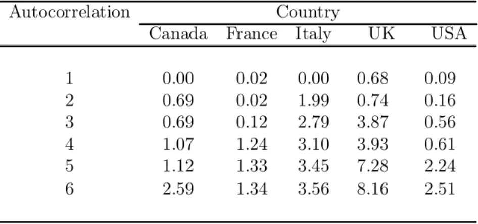
the instrumental variable estimator proposed by Pagan and Ullah cannot be employed in this case because the current endogenous variable is a function of all past history and no instruments are available. Instead, Pagan and Ullah (p. 99) suggest speci¯cation tests to assess whether the chosen ARCH model is valid. A standard misspeci¯cation test for ARCH models is the Ljung-Box Q-statistic applied to the standardized residuals squared. If the ARCH model is correctly speci¯ed, then the residuals corrected for heteroskedasticity and squared should be serially uncorrelated. Table 3 reports the Q-statistic for up to six autocorrelations for all countries. Since all statistics are below the 5% critical value of the appropriate distribution, the null hypothesis of no autocorrelation cannot be rejected at the 5% level. Hence, it would appear that the parsimonious GARCH(1,1) model employed here adequately captures the conditional heteroskedasticity present in the unemployment data.
4
Summary and Discussion
This paper examines, both analytically and empirically, the notion that an in°ation bias can arise in a setup where a central banker with asymmetric preferences targets the natural unemployment rate. Using a model where the natural rate varies over time and a preference speci¯cation that includes the quadric loss function as a special case, it shows that the basic insight in Kydland and Prescott (1977) and Barro and Gordon (1983) is robust to allowing the monetary authority to target the natural rate. A basic time-series prediction of the model is that in°ation and the conditional variance of unemployment are positively related. Maximum Likelihood estimates of the reduced-form parameters support this hypothesis for the United States and France, but not for Canada, Italy, or the United Kingdom. Although the preference parameter that measures the asymmetry in unemployment preferences is not identi¯ed, results are consistent with the view that positive unemployment deviations from the target are weighted more severely than negative ones in the central banker's loss function. In interpreting these empirical results, one must keep in mind some limitations of the game-theoretical model. First, preference parameters (including the in°ation target ¼¤)
could change over time as di®erent individuals take o±ce, and institutional arrangements are revised. For example, it is possible that the reduction in the in°ation rate in the 1990's is not only due to the smaller variability of the unemployment rate but also to institutional changes like the introduction of explicit in°ation targets. Second, the unemployment
per-sistence is only due to the perper-sistence in the natural rate. A more general model would allow, for example, hysteresis in unemployment or an explicit role for technological or busi-ness cycle variables. Lockwood and Philippopoulos (1994) consider a model where lagged unemployment a®ects the current natural rate. Unfortunately, when coupled with the more general preference speci¯cation employed here, the model has no closed-form solution. Fi-nally, although the model allows for the strategic interaction of the public and the central banker, equilibrium concepts other than Nash might be empirically important. Future work seeks to address this limitations, but the results reported above are suggestive of the role of asymmetric preferences in real-world monetary policy making.
Table 1. Univariate Analysis of the Unemployment Rate Country
Canada France Italy Japan UK USA A. Unit Root Tests
ADF ¡1:68 ¡1:40 ¡1:04 0:62 ¡1:83 ¡2:88y
PP ¡1:48 ¡1:45 ¡1:34 ¡2:09 ¡1:37 ¡2:09 B. LM Tests for Neglected ARCH
1 lag 9:11¤¤ 3:90¤ 2:26 0:01 13:85¤¤ 11:70¤¤
2 lags 11:96¤¤ 7:25¤ 5:31y 1:15 14:07¤¤ 16:51¤¤ 3 lags 12:41¤¤ 7:61y 6:02 1:23 14:69¤¤ 16:50¤¤ 4 lags 13:34¤¤ 8:28y 6:55 1:19 14:63¤¤ 16:47¤¤
Notes: ADF and PP stand for Augmented Dickey-Fuller and Phillips-Perron, respectively. The LM statistics were calculated as the product of the number of observations and the uncentered R2 of the OLS regression of the squared unemployment residual on a constant
and one, two, three and four of its lags. Under the null hypothesis of no conditional heteroskedasticity, the statistic is distributed chi-square with as many degrees of freedom as squared residuals are included in the regression. The superscripts ¤¤; ¤, and y denote the
Table 2. ML Estimates
Parameter Country
Canada France Italy UK USA
A. In°ation Process a 4:08¤¤ 2:06¤ 9:31¤¤ 6:27¤¤ 3:08¤¤ (0:60) (1:03) (0:72) (0:80) (0:40) b 5:05 111:08¤¤ 1:60 17:79 15:38¤ (5:56) (36:00) (4:10) (28:96) (6:70) ¾² 3:61¤¤ 3:60¤¤ 5:87¤¤ 5:79¤¤ 2:34¤¤ (0:21) (0:25) (0:38) (0:33) (0:14) B. Conditional Variance of Unemployment
¹ 0:04¤¤ 0:003¤ 0:04¤¤ 0:01¤¤ 0:01¤¤ (0:01) (0:001) (0:01) (0:003) (0:003) ® 0:23¤ 0:12¤¤ 0:38y 0:32¤ 0:23¤ (0:11) (0:04) (0:18) (0:13) (0:10) ! 0:38¤¤ 0:80¤¤ 0:32 0:04 0:64¤¤ (0:14) (0:06) (0:17) (0:14) (0:11) C. Unemployment Process à ¡0:03 0:01 0:06¤ ¡0:01 ¡0:04¤ (0:03) (0:01) (0:03) (0:01) (0:02) µ1 0:49¤¤ 0:71¤¤ ¡0:04 0:83¤¤ 0:64¤¤ (0:09) (0:07) (0:12) (0:04) (0:09) µ2 0:20¤ ¡0:08 (0:09) (0:09) µ3 0:11 0:08 (0:08) (0:10) µ4 ¡0:23¤ ¡0:17¤¤ (0:09) (0:08)
Notes: The conditional variance of the unemployment follows the GARCH(1,1) process: wt = phtºt;where wt is the unemployment disturbance, ºt is an i:i:d sequence with unit
Table 3. Q-Statistic for Autocorrelation Standardized Squared Residuals of Unemployment
Autocorrelation Country
Canada France Italy UK USA
1 0:00 0:02 0:00 0:68 0:09 2 0:69 0:02 1:99 0:74 0:16 3 0:69 0:12 2:79 3:87 0:56 4 1:07 1:24 3:10 3:93 0:61 5 1:12 1:33 3:45 7:28 2:24 6 2:59 1:34 3:56 8:16 2:51
Notes: under the null hypothesis of no autocorrelation, the Q-statistic is distributed chi-square with degrees of freedom equal to the number of autocorrelations.
References
[1] Barro, R. and Gordon, D. (1983), \A Positive Theory of Monetary Policy in a Natural Rate Model," Journal of Political Economy, 91: 589-610.
[2] Blinder, A. S. (1998), Central Banking in Theory and Practice, The MIT Press: Cam-bridge.
[3] Bollerslev, T. (1986), \Generalized Autoregressive Conditional Heteroskedasticity," Journal of Econometrics, 31: 307-327.
[4] Broadbent, B. and Barro, R. J. (1997), \Central Bank Preferences and Macroeconomic Equilibrium," Journal of Monetary Economics, 39: 17-44.
[5] Clarida, R., Gal¶i, J., and Gertler, M. (1999), \The Science of Monetary Policy: A New Keynesian Perspective," Journal of Economic Literature, 37: 1661-1707.
[6] Cukierman, A. (2000), \The In°ation Bias Result Revisited ," Tel-Aviv University, Mimeo.
[7] Dolado, J. J., Mar¶ia-Dolores, R., and Naveira, M. (2000), \Asymmetries in Monetary Policy Rules," Universidad Carlos III, Mimeo.
[8] Engle, R. F. (1982), \Autoregressive Conditional Heteroskedasticity with Estimates of the Variance of United Kingdom In°ation," Econometrica, 50: 987-1007.
[9] Gerlach, S. (1999), \Supply Shocks, Asymmetric Policy Preferences and Excess In°a-tion," Bank for International Settlements, Mimeo.
[10] Gerlach, S. (2000), \Asymmetric Policy Reactions and In°ation," Bank for International Settlements, Mimeo.
[11] Hamilton, J. D. (1996), \This is what Happened to the Oil Price-Macroeconomy Rela-tionship," Journal of Monetary Economics, 38: 215-220.
[12] Ireland, P. N. (1999), \Does the Time-Consistency Problem Explain the Behavior of In°ation in the United States?", Journal of Monetary Economics, 44: 279-291.
[13] King, M. (1996), \How Should Central Banks Reduce In°ation: Conceptual Issues" in Achieving Price Stability, Federal Reserve Bank of Kansas City.
[14] Kydland, F. and Prescott, E. (1977), \Rules Rather Than Discretion: The Inconsistency of Optimal Plans," Journal of Political Economy, 85: 473-490.
[15] Lockwood, B. and Philippopoulos, A. (1994), \Insider Power, Unemployment Dynamics and Multiple In°ation Equilibria," Economica, 61: 59-77.
[16] McCallum, B. T. (1995), \Two Fallacies Concerning Central Bank Independence," American Economic Review Papers and Proceedings, 85: 201-211.
[17] McCallum, B. T. (1997), \Crucial Issues Concerning Central Bank Independence," Jour-nal of Monetary Economics, 39: 99-112.
[18] Nobay, R. A. and Peel, D. A. (1998), \Optimal Monetary Policy in a Model of Asym-metric Central Bank Preferences," London School of Economics, Mimeo.
[19] Nobay, R. A. and Peel, D. A. (2000), \Optimal Monetary Policy with a Nonlinear Phillips Curve," Economics Letters, 67: 159-164.
[20] Pagan, A. (1984), \Econometric Issues in the Analysis of Regressions with Generated Regressors," International Economic Review, 25: 221-247.
[21] Pagan, A. and Ullah, A. (1988), \The Econometric Analysis of Models with Risk Terms," Journal of Applied Econometrics, 3:87-105.
[22] Persson, T. and Tabellini, G. (2000), \Political Economics and Macroeconomic Policy," in Handbook of Macroeconomics, edited by J. Taylor and M. Woodford. North-Holland: Amsterdam.
[23] Ruge-Murcia, F. J. (2000), \The In°ation Bias when the Central Banker Targets the Natural Rate of Unemployment," University of Montreal, Mimeo.
[24] Shimer, R. (1998), \Why is the U.S. UnemploymentRate so Much Lower?," NBER Macroeconomics Annual: 33-49.
[25] Skinner, J. (1988), \Risky Income, Life Cycle Consumption, and Precautionary Sav-ings," Journal of Monetary Economics, 22: 237-255.
[26] Varian, H. (1974), \A Bayesian Approach to Real Estate Assessment," in Studies in Bayesian Economics in Honour of L. J. Savage, edited by S. E. Feinberg and A Zellner. North-Holland: Amsterdam.