Forensic Source Camera Identification by Using Features in Machine Learning Approach

HAL Id: tel-02083780

https://tel.archives-ouvertes.fr/tel-02083780

HAL is a multi-disciplinary open access archive for the deposit and dissemination of sci-entific research documents, whether they are pub-lished or not. The documents may come from teaching and research institutions in France or abroad, or from public or private research centers.

L’archive ouverte pluridisciplinaire HAL, est destinée au dépôt et à la diffusion de documents scientifiques de niveau recherche, publiés ou non, émanant des établissements d’enseignement et de recherche français ou étrangers, des laboratoires publics ou privés.

in Machine Learning Approach

Amel Tuama Alhussainy

To cite this version:

Amel Tuama Alhussainy. Forensic Source Camera Identification by Using Features in Machine Learn-ing Approach. Other [cs.OH]. Université Montpellier, 2016. English. �NNT : 2016MONTS024�. �tel-02083780�

Préparée au sein de l’école doctorale I2S

Et de l’unité de recherche LIRMM

Spécialité: Informatique

Présentée par Amel Tuama ALHUSSAINY

Forensic Source Camera

Identification Using

Features: a Machine

Learning Approach

Soutenue le 1 Decembre 2016 devant le jury composé de

M.Jérôme Azé Pr Université de Montpellier Président de Jury M.Patrick Bas DR-CNRS Université de Lille Rapporteur M.Alessandro Piva Associate Pr Université de Florence (Italie) Rapporteur M.F. Pérez-Gonzàlez Pr Université de Vigo (Espagne) Examinateur M.Marc Chaumont Mcf-HDR Université de Nîmes Directeur de thése M.Frédéric Comby Mcf Université de Montpellier Co-Encadrant M.Alexis Joly Mcf-HDR Université de Montpellier Invité

Forensic Source Camera Identification by Using Features

in Machine Learning Approach

Abstract:

Source camera identification has recently received a wide attention due to its im-portant role in security and legal issue. The problem of establishing the origin of digital media obtained through an imaging device is important whenever digital content is presented and is used as evidence in the court. Source camera identifi-cation is the process of determining which camera device or model has been used to capture an image.

Our first contribution for digital camera model identification is based on the ex-traction of three sets of features in a machine learning scheme. These features are the co-occurrences matrix, some features related to CFA interpolation ar-rangement, and conditional probability statistics computed in the JPEG domain. These features give high order statistics which supplement and enhance the iden-tification rate. The experiments prove the strength of our proposition since it achieves higher accuracy than the correlation-based method.

The second contribution is based on using the deep convolutional neural networks (CNNs). Unlike traditional methods, CNNs can automatically and simultaneously extract features and learn to classify during the learning process. A layer of preprocessing is added to the CNN model, and consists of a high pass filter which is applied to the input image. The obtained CNN gives very good performance for a very small learning complexity. Experimental comparison with a classical two steps machine learning approach shows that the proposed method can achieve significant detection performance. The well known object recognition CNN models, AlexNet and GoogleNet, are also examined.

Keywords:

Identification d’appareils photos par apprentissage

Résumé :

L’identification d’appareils photos a récemment fait l’objet d’un grand intérêt en raison de son apport au niveau de la sécurité et dans le cadre juridique. Établir l’origine d’un média numérique obtenu par un appareil d’imagerie est important à chaque fois que le contenu numérique est présenté et utilisé comme preuve devant un tribunal. L’identification d’appareils photos consiste à déterminer la marque, le modèle, ou l’équipement qui a été utilisé pour prendre une image.

Notre première contribution pour l’identification du modèle d’appareil photo numé-rique est basée sur l’extraction de trois ensembles de caractéristiques puis l’uti-lisation d’un apprentissage automatique. Ces caractéristiques sont la matrice de co-occurrences, des corrélations inter-canaux mesurant la trace laissée par l’inter-polation CFA, et les probabilités conditionnelles calculées dans le domaine JPEG. Ces caractéristiques donnent des statistiques d’ordre élevées qui complètent et améliorent le taux d’identification. La précision obtenue est supérieure à celle des méthodes de référence dans le domaine basées sur la corrélation.

Notre deuxième contribution est basée sur l’utilisation des CNNs. Contrairement aux méthodes traditionnelles, les CNNs apprennent simultanément les caractéris-tiques et la classification. Nous proposons d’ajouter une couche de pré-traitement (filtre passe-haut appliqué à l’image d’entrée) au CNN. Le CNN obtenu donne de bonne performance pour une faible complexité d’apprentissage. La méthode pro-posée donne des résultats équivalents à ceux obtenus par une approche en deux étapes (extraction de caractéristiques + SVM). Par ailleurs, nous avons examinés les CNNs : AlexNet et GoogleNet. GoogleNet donne les meilleurs taux d’identifi-cation pour une complexité d’apprentissage plus grande.

Mots clés :

My mother, your spirit is always with me pushing me

forward.

I am grateful for Almighty Allah for giving me the strength and ability to fulfill this goal. My sincere appreciation and gratitude goes to my primary supervisor Dr. Marc Chaumont for his continuous and valuable advice and guidance, especially the constructive feedback on my thesis. My gratitude is also extended to my co-supervisor Dr. Frédéric Comby for his time, effort and helpful guidance. Also, I would like to thank my examination committee: Professor Patrick Bas, Professor Alessandro Piva, Professor Frenando Pérez-Gonzàlez, Professor Jérôme Azé and Dr. Alexis Joly for their time and efforts.

I dedicate great thanks with love to my wonderful family, my husband Hasan Abdulrahman who taught me a great deal on both personal and professional levels. "I could not have achieved this without you by my side all the time". My lovely and beautiful daughter Dalya, thank you for your nonstop encouragement and understanding.

My friends, it is a blessing to have you in my life. Many thanks are also due to the administration staff in LIRMM laboratory, and all the members of the ICAR team for being such nice and cooperative.

Finally, I would like to thank The Iraqi Ministry of Higher Education and scientific research and the Iraqi Northern Technical University for funding my PhD thesis.

List of Figures 9

List of Tables 10

1 Introduction 2

1.1 Introduction . . . 4

1.2 Digital Forensics . . . 5

1.3 Image Authentication and Tamper detection . . . 6

1.4 Image Source Identification . . . 8

1.5 Thesis Objectives and Contributions . . . 9

1.6 Thesis Outline. . . 10

2 Image Source Identification 12 2.1 Introduction . . . 14

2.2 Distinguishing between Acquisition Devices. . . 15

2.3 Exif Header of the image . . . 16

2.4 Camera pipeline and image formation . . . 17

2.5 State of the Art . . . 19

2.6 Methods based on a correlation test and mathematical model. . . . 20

2.6.1 Sensor Pattern Noise . . . 21

2.6.1.1 Extracting PRNU . . . 22

2.6.1.2 Denoising Filter. . . 23

2.6.2 Sensor Pattern Dust . . . 24

2.6.3 Lens imperfections . . . 25

2.6.4 CFA pattern and Interpolation . . . 27

2.6.5 Camera Identification based Statistical Test . . . 29

2.7 Methods based on feature extraction and machine learning . . . 29

2.8 Conclusion . . . 31

3 Deep Convolutional Neural Networks 32 3.1 Introduction . . . 34

3.2 Classification by Support Vector Machine. . . 35

3.2.1 The curse of dimensionality and Overfitting problem . . . . 36

3.3 Convolutional Neural Networks CNNs. . . 37

3.3.1 Convolutional layer . . . 38 6

3.3.2 Activation function . . . 39

3.3.3 Pooling . . . 39

3.3.4 Classification by Fully connected layers . . . 40

3.3.5 Learning process and Back-propagation algorithm . . . 40

3.3.6 Drop-out technique . . . 41

3.4 Examples of CNNs . . . 42

3.5 Conclusion . . . 44

4 Source Camera Model Identification Using Features from Pol-luted Noise 45 4.1 Introduction . . . 47

4.2 Correlation method for camera identification (PRNU) . . . 48

4.3 Proposed Machine Learning Feature Based Method . . . 49

4.3.1 Polluted sensor noise extraction . . . 49

4.3.2 Feature set 1: Co-occurrences Matrix . . . 51

4.3.3 Feature set 2: Color Dependencies. . . 52

4.3.4 Feature set 3: Conditional Probability . . . 53

4.4 Experimental Results . . . 54

4.4.1 Dresden image database . . . 54

4.4.2 Experimental setting . . . 55

4.4.2.1 Comparison with another feature based method . . 57

4.4.2.2 Comparison with Correlation based method . . . . 58

4.4.2.3 Robustness test against the overfitting . . . 58

4.5 Conclusion . . . 60

5 Camera Model Identification Based on a CNN 61 5.1 Introduction . . . 63

5.2 The Proposed CNN Design for Camera Model Identification . . . . 64

5.2.1 Filter layer . . . 64

5.2.2 Convolutions . . . 65

5.2.3 Fully Connected layers . . . 66

5.3 Dataset organizing . . . 66

5.4 System requirements . . . 68

5.5 Experiments and Results . . . 68

5.6 Comparison with AlexNet and GoogleNet . . . 70

5.7 Conclusion . . . 71

6 Conclusions and Perspectives 73 6.1 Conclusions . . . 75

6.2 Perspectives and Open Issues . . . 76

7 Résumé en Francais 77 7.1 Introduction . . . 79

7.2 Identification du modèle de caméra par utiliser de caractéristiques calculées sur le bruit pollué . . . 81

7.3 Identification du modèle de caméra basée sur un CNN. . . 82

7.4 Conclusion . . . 83

8 List of Publications 85

8.1 List of Publications . . . 87

1.1 Hierarchy of digital image forensics. . . 5

1.2 Example of a tampered image: (a) The original picture of Ross Brawn receiving the Order of the British Empire from the queen Elizabeth II. (b) The tampered image depicting Jeffrey Wong Su En while receiving the award from the queen. The image was taken from [AWJL11]. . . 7

2.1 Types of acquisition devices. . . 15

2.2 Some of the EXIF details. . . 16

2.3 Image formation pipeline . . . 17

2.4 Camera levels, brand, model, Device. . . 19

2.5 Camera Identification methods. . . 20

2.6 Denoising filter applied on a color image (a) the image , (b) denoised image of the red channel, (c) denoised image of the green channel, (d) denoised image of the blue channel. . . 24

2.7 Dark spots in the white square are the sensor dust particles. The image was taken from [DSM08] . . . 25

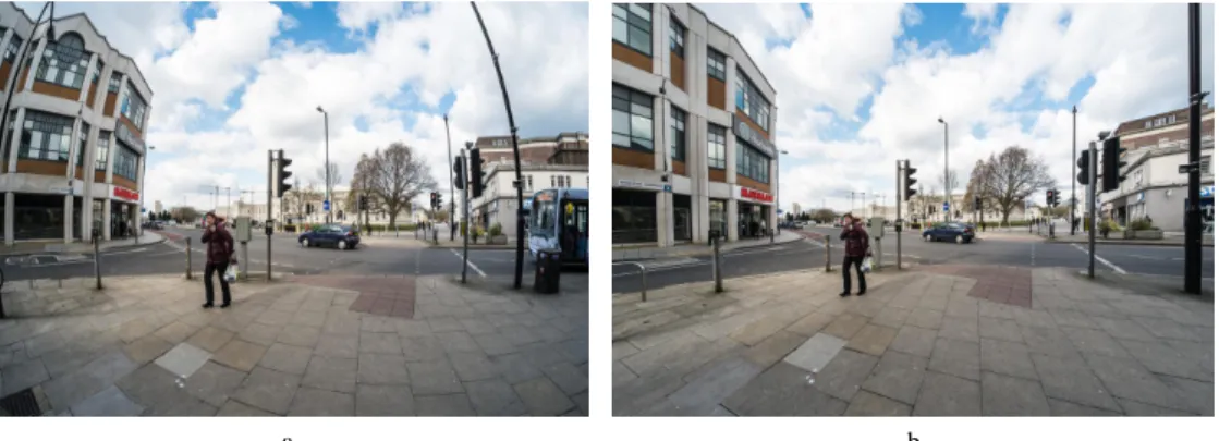
2.8 The distortion is clear in the first image. . . 26

2.9 Lens Radial distortion types (a)undistorted shape(b)barrel distor-tion(c)pincushion distortion . . . 26

2.10 Color filter array patterns . . . 28

3.1 The Conventional neural networks concept . . . 38

3.2 AlexNet CNN model with the use of 2 GPUs. Image is extracted from [KSH12] . . . 42

3.3 The layout of GoogleNet. Image is extracted from [SLJ+_{15] . . . . 43}

4.1 The correlation based scheme . . . 48

4.2 The proposed system framework . . . 49

4.3 Example of a denoised image. . . 50

4.4 Eight different arrangements of r, s, t coefficients . . . 54

4.5 Comparison of the identification results. . . 59

5.1 The layout of our Conventional Neural Networks for Camera Model Identification. . . 64

7.1 Pipeline d’un appareil photo . . . 79 9

2.1 A comparison between feature based camera identification methods. 31

3.1 Kernel function types of SVM classifier.. . . 35

4.1 Camera models used from Dresden database. . . 55

4.2 Identification accuracy of the proposed method and the correlation based method for 14 chosen camera models. . . 56

4.3 Results of the proposed method with comparison to another methods. 57

4.4 Test results for images from Flickr data set. . . 60

5.1 Camera models used in the experiments, models marked with * comes from personal camera models while all the others are from Dresden database.. . . 67

5.2 Identification accuracy (in percentage points %) of the proposed method for Residual1, the total accuracy is 98%. − means zero or less than 0.1. . . 69

5.3 results for the first 12 camera models considering the pooling layer for Residual1. . . . 70

5.4 Identification accuracies for all the experiments compared to AlexNet and GoogleNet. . . 71

Introduction

Contents

1.1 Introduction . . . . 4

1.2 Digital Forensics . . . . 5

1.3 Image Authentication and Tamper detection . . . . 6

1.4 Image Source Identification . . . . 8

1.5 Thesis Objectives and Contributions . . . . 9

1.6 Thesis Outline . . . 10

1.1

Introduction

Today, multimedia (image, audio, video, etc) proceeds fast and spreads into all areas of human life. Frequent use of multimedia brings some new issues and challenges about its authenticity and reliability. Recent studies in multimedia forensics have begun to develop techniques to test the reliability and admissibility of multimedia.

In general, an evidence refers to information or objects that may be admitted into court for judges and juries to consider when hearing a case. An evidence can serve many roles in an investigation, such as to trace an illicit substance, identify remains or reconstruct a crime. The digital evidence is information stored or transmitted in binary form. It can be found on a computer hard drive, a mobile phone, a CD, and a flash card in a digital camera. For example, suspects e-mail or mobile phone files might contain critical evidence regarding their intent, their whereabouts at the time of a crime and their relationship with other suspects. For example, in 2005, a floppy disk led investigators to a serial killer who had eluded police capture since 1974 and claimed the lives of at least 10 victims [Jus15]. One of the multimedia elements is the digital image which is a very common evidence. An image (a photograph) is generally accepted as a proof of occurrence of the depicted event. As a way to represent a unique moment in space-time, digital images are often taken as silent witnesses in the court of law and are a crucial piece of crime evidence. Verifying a digital image integrity and authenticity is an important task in forensics especially considering that the images can be digitally modified by low-cost hardware and software tools that are widely available [TN08]. Section 1.2 of this chapter gives a definition and brief introduction about Digital Forensics. Image authentication and tamper detection is introduced in Section

1.3. A brief introduction to camera identification is given in Section 1.4. The objectives and contributions of this thesis will be presented in Section 1.5. The whole layout of this thesis is given in Section 1.6.

1.2

Digital Forensics

The first definition for digital forensics science has been formulated in 2001 during the first Digital Forensic Workshop [DFR01]. This definition was exactly: "The

use of scientifically derived and proven methods toward the preservation, collection, validation, identification, analysis, interpretation, documentation and presentation of digital evidence derived from digital sources for the purpose of facilitating or furthering the reconstruction of events found to be criminal, or helping to anticipate unauthorized actions shown to be disruptive to planned operations".

Digital forensics can simply be defined as the discipline that combines elements of law and computer science to collect and analyze data from computer systems, networks, wireless communications and storage devices in a way that is admissible as evidence in a court of law. In particular, digital forensics science emerged in the last decade in response to the escalation of crimes committed by the use of electronic devices as an instrument used to commit a crime or as a repository of evidences related to a crime [ACC+_10].

The digital evidence is any probative information stored or transmitted in digital

form that a party to a court case may use at trial [Cas04]. Digital forensics, as

Active Forensic Techniques

Digital Image Forensics

Passive Forensic Techniques

Watermarking Digital Signature Tamper Detection _{Identification}Source

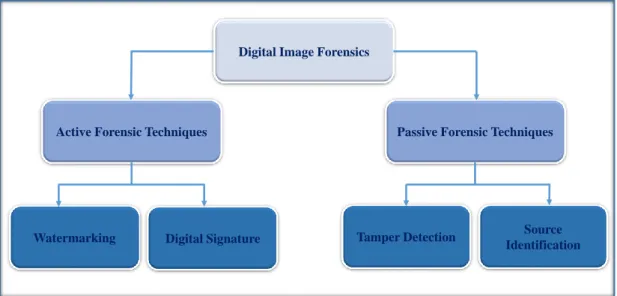
illustrated in Figure 1.1, is divided into active and passive techniques. In the active forensic techniques, it is necessary to operate on the original document which has to be available from the beginning like in the watermarking or digital signature. While the passive forensic is a technique that can operate with no prior information about the content is available or no integrity protection mechanisms. It is straightforward to realize that this kind of investigation has to be founded on the thorough analysis of some intrinsic features that may be present inside the observed data [CH04].

Digital image forensics research aims at uncovering underlying facts about an image. It covers the answers to many questions such as:

• Can we trust an image?

• Is it original image or manipulated by some image processing tool? • Was it generated by a digital camera, mobile phone, or a scanner? • What is the brand and model of the source used to capture the image?

In digital image forensics, there are two main challenges. The first one is the source identification which makes possible to establish a link from the image to its source device, model, or brand. In tracing the history of an image, identifying the device used for its acquisition is of major interest. In a court of law, the origin of a particular image can represent a crucial evidence. The second challenge related to the detection of forgeries. In this case, it is required to establish if a certain image is authentic, or if it has been artificially manipulated in order to change its content [TN08].

1.3

Image Authentication and Tamper detection

With the rapid diffusion of electric imaging devices that enable the acquisition of visual data, almost everybody has today the possibility of recording, storing, and

sharing a large amount of digital images. At the same time, the large availability of image editing software tools makes extremely simple to alter the content of the images, or to create new ones, so that the possibility of tampering and modifying visual content is no more restricted to experts.

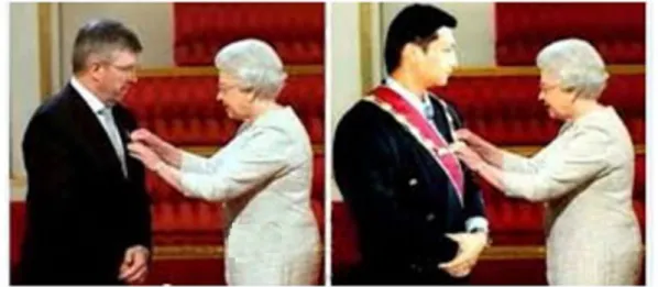
Tampering is any processing operation that is applied on a multimedia object after it has been created. Tampering can be divided to two types: innocent and malicious. Innocent tampering may modify the image quality in the time it doesn’t change the contents of the image. This includes various operations such as contrast adjustment, brightness adjustment, up-sampling, downsampling, zooming, rotation etc. While malicious tampering aims at modifying the contents of the image and may includes operations such as cut-paste, copy-paste, region cloning and splicing [Ale13] as in the example illustrated in Figure 1.2.

Figure 1.2: Example of a tampered image: (a) The original picture of Ross Brawn receiving the Order of the British Empire from the queen Elizabeth II. (b) The tampered image depicting Jeffrey Wong Su En while receiving the award

from the queen. The image was taken from [AWJL11].

Though existing digital forensic techniques are capable of detecting several stan-dard digital media manipulations, they do not account for the possibility that may be applied to digital content. In reality, it is quite possible that a forger may be able to secretly develop anti-forensic operations and use them to create undetectable digital forgeries.

Anti-forensic or counter forensics operations designed to hide traces of manip-ulation and editing fingerprints resulted from forensic techniques. Research on counter-forensics is motivated by the need to assess and improve the reliability of forensic methods in situations where intelligent adversaries make efforts to induce a certain outcome of forensic analyses [BK13].

Furthermore, the study of anti-forensic operations can also lead to the identifica-tion of fingerprints left by anti-forensic operaidentifica-tions and the development of tech-niques capable of detecting when an anti-forensic operation has been used to hide evidence forgery. It is clear that the authentication of multimedia signals poses a great challenge to information security researchers [Ale13].

1.4

Image Source Identification

As seen previously, source identification for digital content is one of the branches of digital image forensics. It aims at establishing a link between an image and its acquisition device by exploiting traces left by the different steps of the image acquisition process. Currently, the forensic community has put some efforts into the identification of images which may be generated by a digital camera, mobile phone, or even a scanner.

The authenticity of an image under investigation can be enforced by identifying its source. Source attribution techniques aim at looking for scratches left in an image by the source camera. These marks can be caused by factory defects, or the interaction between device components and the light.

In the source identification, the basic assumption is that digital contents are over-laid by artifacts added by the internal components of the acquisition device. Such artifacts are invisible to the human eye, but it can be analyzed to successfully contribute in the identification process. Source camera identification techniques achieve two major axes. The first one is searching for the properties of the camera

model, and the second is identifying the individual camera device [KG15]. The two axes will be explained in Chapter 2.

1.5

Thesis Objectives and Contributions

In this thesis, the subject of source device identification has been studied. In particular two different techniques will be presented in the following chapters. For each method, we describe all the conditions and details, and bring out the experiments and results that validate the methodology. The general aims and objectives of this thesis are as follows:

• Propose and analyze a technique for digital source camera model identifi-cation based on classical feature extraction and machine learning approach [TCC16a, TCC16b].

• Propose and implement the deep learning approach to enhance a CNN model for camera model identification.

• Investigate and demonstrate the state-of-the-art techniques related to source identification showing the limitations of each method.

• Compare our proposed methods performance with similar state-of-the-art techniques either in classical approach or in CNN approach.

1.6

Thesis Outline

This thesis is outlined as follows:

• Chapter2briefly highlight the recent state-of-the-art techniques for the cam-era identification forensics. Also we show a brief look to camcam-era pipeline since it gives clues on where to find specific features in the acquisition process. Some traces are left that can be identified (or at least tried to be identified). The relationship with tamper detection and Anti-forensic is discussed. • Chapter 3 discusses the global term for classical machine learning, then it

goes deeper to illustrate the approach of deep learning and convolutional neural networks. Some details of Support Vector Machine are discussed. • Chapter 4 describes the development of a method for digital camera model

identification by extracting three sets of features in a machine learning scheme. These features are the co-occurrences matrix, some features related to CFA interpolation arrangement, and conditional probability statistics. • Chapter5presents a new method of camera model identification using CNN

approach. All the details of the proposed CNN architecture and System requirements are described. The experiments and comparisons with other models are demonstrated.

• Chapter 6summarizes, concludes and discusses future work in camera iden-tification.

Image Source Identification

Contents

2.1 Introduction . . . 14

2.2 Distinguishing between Acquisition Devices . . . 15

2.3 Exif Header of the image . . . 16

2.4 Camera pipeline and image formation . . . 17

2.5 State of the Art . . . 19

2.6 Methods based on a correlation test and mathematical

model . . . 20

2.6.1 Sensor Pattern Noise . . . 21

2.6.2 Sensor Pattern Dust . . . 24

2.6.3 Lens imperfections . . . 25

2.6.4 CFA pattern and Interpolation . . . 27

2.6.5 Camera Identification based Statistical Test . . . 29

2.7 Methods based on feature extraction and machine learning 29

2.8 Conclusion . . . 31

2.1

Introduction

This chapter reviews digital forensic techniques for source camera identification. The tasks for digital multimedia forensics are grouped into six categories as follows [CFGL08]:

• Source Classification: classifies images according to their origin, scanner or camera device.

• Source Identification: searches for identifying a specific camera device, model, or make from a given image.

• Device Linking: links a device with a set of captured images.

• Processing History Recovery: retrieves the image processing steps applied to an image like type of compression method, or filtering.

• Integrity Verification and tamper detection.

• Anomaly Investigation: explaining anomalies found in images.

In our work, we focus on the source identification due to its necessity for legal and security reasons. Image source identification requires well understanding of the physical image formation pipeline. This pipeline is similar for almost all digital cameras, although much of the details are kept as proprietary information of each manufacturer.

This chapter will discuss in details these two groups. We will distinguish between the acquisition devices in the following section 2.2 followed by some details about the Exif Header of the image in the section 2.3. Methods of the first group will be discussed in Section2.6 while the methods supported by machine learning will be discussed in Section 2.7.

2.2

Distinguishing between Acquisition Devices

The well known source of a digital image is the digital camera or cell phone device. Another kind of images that can constitute a digital evidence to be checked, in addition to those ones acquired with a photo camera or with a camcorder, might come from a scanning operation. This means that a printed document located in a flatbed scanner has been illuminated row by row by a sliding mono-dimensional sensor array to originate the digital data [KMC+_{07]. In this case, other elements,}

in addition to those already exist for cameras, can be considered during the forensic analysis process.

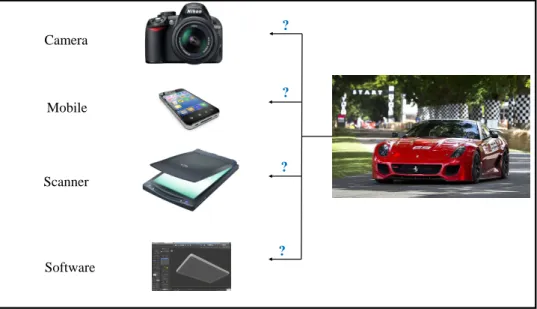
Computer generated graphics could be used to generate digital images since it touch many aspects of daily life. Computer imagery is found on television, in newspapers, and in all kinds of medical investigation and surgical procedures that has brought new challenges towards the originality of digital images. To locate the origin of the image whether it is a photographic or computer generated, image contour information can be extracted, or a correlation between CFA interpolation, or PRNU noise [PZ14]. Figure 2.1 illustrates the possible types of acquisition devices. Mobile Camera Scanner Software ? ? ? ?

In general, most of the techniques for camera identification do not work only for digital cameras but also for scanner and camcorder identification and also to distinguish between a photographic and a computer graphic image [TN08].

2.3

Exif Header of the image

Digital images, can be stored in a variety of formats, such as JPEG, GIF, PNG, TIFF. For example JPEG files contain a well-defined feature set that includes metadata, quantization tables for image compression and lossy compressed data. The metadata usually includes information about the camera type, resolution, focus settings, and other features [Coh07]. Besides when RAW format is used, the camera creates a header file which contains all of the camera settings, including sharpening level, contrast and saturation settings, colour temperature and white balancing.

Figure 2.2: Some of the EXIF details

Although such metadata provide a significant amount of information it has some limitations since they can be edited, deleted and false information can be inserted about the camera type and settings. Normally, metadata or ’EXIF’ header, refers to Exchangeable Image File Format, is considered the simplest way to identify an image source. It provides a standard representation of digital images as in Figure

2.2. Since the ’EXIF’ headers can be easily modified or destroyed so we cannot rely on their information [TN08].

2.4

Camera pipeline and image formation

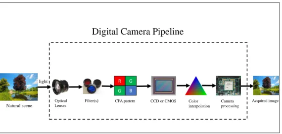
The general structure of a digital camera pipeline remains similar in all digital cameras. The exact processing detail in each stage varies from one manufacturer to the other, and even in different camera models manufactured by the same company. Figure 2.3 describes the basic structure for a digital camera pipeline. Digital Camera Pipeline consists of a lens system, optical filters, color filter array, imaging sensor, and a digital image processor.

Optical Lenses

Filter(s) CCD or CMOS

Digital Camera Pipeline

Natural scene light Color interpolation Camera processing

CFA pattern Acquired image

R G B

G

Figure 2.3: Image formation pipeline

• The lens system: It is essentially composed of a lens and the mechanisms to control exposure, focusing, and image stabilization to collect and control the light from the scene.

• Optical filters: After the light enters the camera through the lens, it goes through a combination of interposed optical filters that reduces undesired light components (e. g., infrared light).

• The imaging sensor: It is an array of rows and columns of light-sensing el-ements called photo-sites. In general there are two types of camera sensors deployed by digital cameras, the charge-coupled device (CCD) or compli-mentary metal-oxide semiconductor (CMOS). Each light sensing element of

sensor array integrates the incident light over the whole spectrum and ob-tains an electric signal representation of the scenery.

• CFA array: Since each imaging sensor element is essentially monochromatic, capturing color images requires separate sensors for each color component. However, due to cost considerations, in most digital cameras, only a single sensor is used along with a color filter array (CFA). The CFA arranges pixels in a pattern so that each element has a different spectral filter. Hence, each element only senses one band of wavelength, and the raw image collected from the imaging sensor is a mosaic of different colors and varying intensity values. The CFA patterns are most generally comprised of red-green-blue (RGB) color components.

• Demosaicing operation: As each sub-partition of pixels only provide infor-mation about a number of color component values, the missing color values for each pixel need to be obtained through demosaicing operation by inter-polating three colors at each pixel location.

• Digital image processing: It is a series forms of image processing like white point correction, image sharpening, aperture correction, gamma correction and compression [KG15]. The colors are corrected, converting them from white balanced camera responses into a set of color primaries appropriate for the finished image. This is usually accomplished through multiplication with a color correction matrix. Edge enhancement or sharpening is applied on the image to reduce high spatial frequency content and improve the appearance of images. Once an image is fully processed, it is often compressed in one of the two compression algorithms; lossy and lossless. This step is important to reduce the amount of physical storage space required to represent the image data [AMB13].

2.5

State of the Art

In the literature of source identification, there are techniques that have investigated the presence of a specific CFA pattern in the image texture and other methods which have proposed to analyze the anomalies left by the device over the image such as scratches on the lenses, or defective pixels. In the other hand, big attention has paid to the defects of the sensor and dark current with what so called PRNU (Photo Response Non-Uniformity) which is one of the most interesting methods for forensic applications. While the other approaches use a set of data intrinsic features designed to classify camera models.

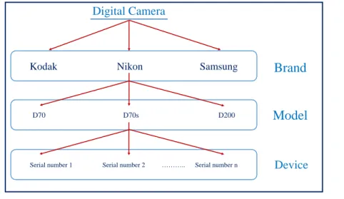
In source camera identification, it is necessary to distinguish between the levels of brand, model, and device. In order to well understand this hierarchical classifi-cation of cameras, in the first level of nomination process comes the name of the brand or manufacturer like the "Kodak" or "Nikon". The camera model comes in the second level such that models share most of the basic properties like the CFA pattern or lenses type and design. In the bottom of the classification hierarchy, we can see the individual digital cameras of the same model. Figure 2.4 shows these different levels with example from "Nikon" manufacturer.

D70 D70s D200

Brand

Model

Device Digital Camera

Serial number 1 Serial number 2 ……….. Serial number n Kodak Nikon Samsung

Figure 2.4: Camera levels, brand, model, Device.

Camera identification techniques are expected to achieve two major axes. The first extracts the model properties of the source, and the second is to identify the

individual source properties. Camera identification techniques based on sensor dust and sensor noise are only used for device identification while all the other methods are used for model identification [AWJL11].

We already classified the methods for identifying camera device into two main groups. The first group searches in camera identification through passing an sta-tistical test between camera device and an image of unknown source. While the second group collects specific features from the image to deal with in a machine learning pool as shown in figure 2.5.

Methods Based on Correlations or mathematical model Methods Based on Feature extraction & machine

learning

METHODS FOR CAMERA IDENTIFICATION

 Color Features  Image Quality Metrics  Binary Similarity Measures  Conditional Probability  Wavelet Statistics  Local Binary Patterns  Sensor Pattern Noise

 Sensor Pattern Dust  Lens Imperfections

Figure 2.5: Camera Identification methods.

2.6

Methods based on a correlation test and

math-ematical model

This set of methods is based on producing a mathematical model in order to extract a relation between the image and the source. The image acquisition process involves many steps inside camera device which add artifacts to the image content. These artifacts can contribute in providing different features for the identification process. The techniques under consideration aim at analyzing those features in order to find a fingerprint for the device due to the sensor imperfections (dust and

noise), or lens aberrations. As a result the fingerprint of the camera is independent of the content of the analyzed data.

2.6.1

Sensor Pattern Noise

The imaging sensor consists of an array of rows and columns of light-sensing el-ements called photo-sites which are made of silicon. Each pixel integrates the incident light and converts photons into electrons by using analog to digital con-verter. There are many types of noise that comes from different factors including the imperfections in manufacturing process, silicone in-homogeneity, and thermal noise. The most significant one is the pattern noise. It is unique for each camera device which make it the only tool to identify an individual device. There are two main components of the pattern noise:

• The fixed pattern noise (FPN) is caused by dark currents when the sensor array is not exposed to light. It is an additive noise, so it is suppressed automatically by subtracting a dark frame from the captured image.

• The photo response non uniformity (PRNU) is the major source of noise. It is caused when pixels have different light sensitivities caused by the in-homogeneity of silicon wafers. PRNU is a high frequency multiplicative noise, generally stable over time and it is not affected by humidity and temperature.

The relation between the two types of pattern noise over an image I(x,y) is given in the equation2.6 as follows:

I(x, y) = I0(x, y) + γI0(x, y)K(x, y) + N (x, y) (2.1)

where I0(x, y) is the noise-free image, γ is a multiplicative constant, K(x, y) is the

2.6.1.1 Extracting PRNU

By correlating the noise extracted from a query image against the known reference pattern, or PRNU, of a given camera, we can determine whether that camera was used to originally capture the query image. The reference pattern of a camera is first extracted from a series of images taken from known camera device. The reference pattern is then used to detect whether the camera used to generate the reference pattern was used to capture an unknown source image. Generally, for an image I, the residual noise is extracted by subtracting the denoised version of the image from the image itself as follows:

N = I − F (I), (2.2) where F (I) is the denoised image, and F is a denoising filter. A wavelet based denoising filter is used in most cases [Fri09]. In order to extract the fingerprint of a camera, multiple images are denoised and averaged. The averaging of multiple images reduces the random components and enhances the pattern noise. About 50 images are used to calculate the reference pattern Kdof a known camera device

as in Equation 5.2. Kd = Pn i=1(NiIi) Pn i=1Ii2 . (2.3)

A common approach to perform a comparison is to compute the Normalized Cross-Correlation which measures the similarity between the reference pattern Kd and

the estimated noise N of an image under test which is of unknown source [Fri09]. Normalized Cross-Correlation is defined as:

ρ(N, Kd) =

(N − N ).(Kd− Kd)

kN − N k.kKd− Kdk

. (2.4)

2.6.1.2 Denoising Filter

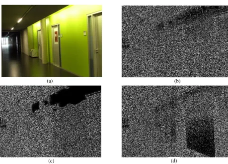
Wavelet based denoising filter in the frequency domain is used in [LFG06] be-cause it gave good results. By applying this particular denoising filter, the noise residual obtained contains the least amount of traces of the image content. The low frequency components of the PRNU signal are automatically suppressed when working with the noise residuals. Basically, this algorithm is composed of two steps. The first step estimates the local variance of the wavelet components, where the second step applies the Wiener filter on the wavelet coefficients [JM04]. An example of the results given by this filter is shown in figure 2.6. The denoising algorithm is as follows:

• Calculate the four level wavelet decomposition of the image using the Daubechies, 8-tap, Separable Quadrate Mirror Filters (QMF). The number of decom-position levels can be increased to improve accuracy or reduced to reduce processing time. At each level, the three high frequency sub-bands are hor-izontal H, vertical V, and diagonal D. For each wavelet sub-band, the local variance in a window of (f × f ) of the neighborhood N is estimated by the formula in equation2.5 as follows:

ˆ σ_f2(i, j) = max

(

)

manually such that σ0 ∈ 1, ..., 6.

The minimum value of the four variances will be taken as the final estimate.

σ2(i, j) = min(σ2₃, σ₅2, σ2₇, σ₉2), (2.6) • The denoised wavelet coefficients are obtained using the Wiener filter men-tioned in equation 2.7 for H, V, and D. Then, apply the inverse wavelet transformation on the denoised wavelet sub-bands to get the denoised com-ponent of the original image.

Iclean(i, j) = I(i, j) ˆ σ2(i, j) ˆ σ2_{(i, j) + σ}2 0 (2.7) (b) (a) (d) (c)

Figure 2.6: Denoising filter applied on a color image (a) the image , (b) denoised image of the red channel, (c) denoised image of the green channel, (d)

denoised image of the blue channel.

2.6.2

Sensor Pattern Dust

This method is related to digital single lens reflex (DSLR) cameras which allow users to work with multiple interchangeable lenses. Once the lens is released, the dust particles are attracted to the camera sensor by electrostatic fields resulting a dust pattern which settles on the protective element at the surface of the sensor [DSM07]. The dust pattern can be seen as small specks, in the form of localized intensity degradations, all over the images produced by this camera device as shown in the Figure 2.7. Sensor dust spots can stay at the same position for very long times unless the sensor is cleaned. The random positions of dust spots create a unique pattern which can be used as a natural fingerprint of a DSLR camera. Dirik et al [DSM08] proposed the dust patterns as a useful fingerprint to identify an individual device. Dust spots in the image are detected based on a Gaussian intensity loss model and shape properties. The shape and darkness of the dust spots are determined by calculating the distance between the dust particle and

imaging sensor. The factors of camera focal length and aperture size are also used to determine the dust particles positions.

Figure 2.7: Dark spots in the white square are the sensor dust particles. The image was taken from [DSM08]

This method is not used with Compact cameras since they do not suffer from sensor dust problem. It is only used with DSLR cameras that need to be changed from time to another. In addition, recent devices come with built-in dust removal mechanisms.

2.6.3

Lens imperfections

Each digital camera is equipped with a specific optical lenses to pass the scene light to the sensor. Most lenses introduce different kinds of lens aberrations such as spherical aberration, field curvature, lens radial distortion and chromatic dis-tortion. Among the Lens aberrations, radial lens distortion is the most grave part [CLW06]

Due to the design process, most lenses introduce geometric distortion where straight lines in real world appear curved in the produced image. Figure 2.8 shows an example of geometrical lens distortion.

The radial distortion causes straight lines in the object space rendered as curved lines on camera sensor and it occurs when there is a change in transverse mag-nification Mt with increasing distance from the optical axis. The degree and the

a b

Figure 2.8: The distortion is clear in the first image.

a b c

Figure 2.9: Lens Radial distortion types (a)undistorted shape(b)barrel dis-tortion(c)pincushion distortion

or even in different camera models by the same manufacturer. As a result, lenses from different cameras share unique fingerprints related to lens on the captured images. Lens radial distortion can be found in two types. The first one is called the barrel distortion, and it happens when Mtincreases with r. The optical system

suffers from pincushion distortion when Mt decreases with r. Example of the two

types of distortion are shown in Figure 2.9.

The general formula of lens radial distortion can be written as in Equation 2.1:

ru = rd+ k1r3d+ k2rd5 (2.8)

where ru and rd are the undistorted radius and distorted radius respectively. The

radius is the radial distance of a point (x, y) from the center of distortion, where

extract the distortion parameters following the Devernay’s straight line method [FO01]. However this method fails if there are no straight lines in the image and also if two cameras of the same model are compared. Besides it is also possible to operate a software correction in order to correct the radial distortion on an image. Another type of aberration is the chromatic aberration which is carried out to identify the source. Chromatic aberration is the phenomenon where light of dif-ferent wave lengths fail to converge at the same position of the focal plane. There are two kind of chromatic aberration: longitudinal aberration that causes different wave lengths to focus at different distances from the lens, while lateral aberration is attributed at different positions on the sensor. In both cases, chromatic aber-ration leads to various forms of color imperfections in the image. Only lateral chromatic aberration is taken into consideration in the method described by Van et al [VEK07] for source identification. This method estimates the distorted pa-rameters to compensate the distortion maximizing the mutual information among the color channels. Mayer et Stamm [MS16] proposed the lateral chromatic aberra-tion for copy-paste forgery detecaberra-tion forensics. The authors proposed a statistical model of the error between local estimates of chromatic aberration displacement vectors and those predicted by a global model.

2.6.4

CFA pattern and Interpolation

Essentially, the sensor is monochromatic such that the capturing of a color image requires putting a color mask in front of the sensor. This is represented by the Color Filter Array (CFA) which it is a color mosaic that covers the imaging sensor. The CFA permits only one color component of light to pass through it at each position before reaching the sensor. Each camera model uses one of several CFA patterns like those shown in figure 2.10. The most common array is the Bayer pattern which uses one red, one blue, and two green. RGBE pattern is used in some models of Sony cameras while CYYM pattern is used in some Kodak models.

RGB 2x2 RGBE 2x2 CYYM 2x2 CYGM 2x2 RGBW 2x2 RGBW 4x4

Figure 2.10: Color filter array patterns

As a result, the sensor records only one particular color value at each pixel location. The two missing color values at each pixel location must be estimated using a process known as demosaicing or color interpolation.

There are several algorithms for color interpolation such that each manufacturer employs a specific algorithm for a specific camera model. The source camera identification techniques are focused on finding the color filter array pattern and the color interpolation algorithm employed in internal processing blocks of a digital camera pipeline that acquired the image.

The approach proposed by Swaminathan et al. [SWL07] based on the fact that most of commercial cameras use RGB type of CFA with a periodicity of 2 × 2. Based on gradient features in a local neighborhood, the authors divided the image into three regions. Then they estimated the interpolation coefficients through singular value decomposition for each region and each color band separately. The sampled CFA pattern is re-interpolated and chose the pattern that minimizes the difference between the estimated final image and actual image produced by the camera.

Bayram et al. in [BSM06] proposed to use the periodicity arrangement in CFA pattern to find a periodic correlation. Expectation Maximization (EM) algorithm is applied to find the probability maps of the observed data to find a relation if exist between an image and a CFA interpolation algorithm. Two sets of features are extracted: the set of weighting coefficients of the image, and the peak locations and magnitudes in frequency spectrum. This method does not work in case of cameras of the same model, because they share the same CFA pattern and interpolation algorithm. Also, it does not work for compressed image, modified by gamma

correction, or smoothing techniques because these artifacts suppress and remove the spatial correlation between the pixels.

2.6.5

Camera Identification based Statistical Test

Another approach for camera identification is the statistical model-based methods. Thai et al. [TRC16] designed a statistical test within hypothesis testing framework for camera model identification from RAW images based on the heteroscedastic noise model. In this scenario, two hypotheses are proposed. The first one assumed that an image belongs to a camera A. While the second hypothesis assumed that the image belongs to a camera B. The parameters (a, b) are proposed to be exploited as camera fingerprint for camera model identification.

In an ideal context where all model parameters are perfectly known, the Likelihood Ratio Test (LRT) is presented and its statistical performances are theoretically established. In practice when the model parameters are unknown, two Generalized Likelihood Ratio Tests (GLRTs) are designed to deal with this difficulty such that they can meet a prescribed false alarm probability while ensuring a high detection performance.

The same statistical approach is used again for camera identification but this time it relies on the camera fingerprint extracted in the Discrete Cosine Transform (DCT) domain based on the state-of-the-art model of DCT coefficients [TRC15]. However, those prior works have the indisputable disadvantage to be unable of distinguishing different devices from the same camera model.

2.7

Methods based on feature extraction and

ma-chine learning

There are other approaches for camera model identification using a set of suitable digital data intrinsic features designed to classify a camera model. The feature

sets could be individual or merged. The promise of merging feature sets is that the resulting feature space provides a better representation of model specific im-age characteristics, and thus gives a higher classification accuracy than individual feature sets.

Kharrazi et al. [KSM04] proposed 34 features from three sets to perform cam-era model identification. The features are color features, Image Quality Metrics (IQM), and wavelet domain statistics. Image quality metrics (IQM) evaluated between an input image and its filtered version using a low-pass Gaussian filter, and integrated with color features (deviation from gray, inter-band correlation, gamma factor), and wavelet coefficient statistics. These features are used to con-struct multi-class classifiers with images coming from different cameras, but it is demonstrated that this approach does not work well with cameras with similar CCD and it requires images of the same content and resolution.

Celiktutan et al. [CSA08] used another group of selected features to distinguish among various brands of cell-phone cameras. Binary similarity measures (BSM), IQM features, and High-Order Wavelet Statistic (HOWS) features are used here to get 592 features.

Filler et al. [FFG08] introduced a camera model identification method using 28 features related to statistical moments and correlations of the linear pattern. Gloe et al. [Glo12] used Kharrazi’s feature sets with extended color features to produce 82 features. Xu and Shi [XS12] used 354 Local Binary Patterns ( or what so-called Ojala histograms) as features. Local binary patterns capture inter-pixel relations by thresholding a local neighborhood at the intensity value of the center pixel into a binary pattern.

Wahab et al. [AHL12] used the conditional probability as a single feature set to classify camera models. The authors considered DCT domain characteristics by exploiting empirical conditional probabilities of the relative order of magnitudes of three selected coefficients in the upper-left 4 × 4 low-frequency bands. The 72-dimensional feature space is composed from conditional probabilities over 8 different coefficient subsets.

Camera Iden. No.of No.of

Method Feature sets Features Models

Kharrazi et al. Color features,IQM,Wavelet features 34 5

(2004) [KSM04]

Celiktutan et al. IQM,Wavelet features,BSM 592 16

(2008) [CSA08]

Filler et al. Statistical moments,Block covariance, 28 17

(2008) [FFG08] Cross-correlation of CFA,

Cross-correlation of linear pattern

Gloe et al. Color features,IQM,Wavelet features 82 26

(2012) [Glo12]

Xu and Shi Local Binary Patterns 354 18

(2012) [XS12]

Wahab et al. Conditional Probability 72 4

(2012) [AHL12]

Marra et al. Spam of Rich models 338 10

(2015) [MPSV15]

Table 2.1: A comparison between feature based camera identification methods.

Marra et al. [MPSV15] used of blind features extraction based on the analysis of image residuals. In this method, authors gathered 338 SPAM features ( linear high pass filters computing derivatives of first to fourth order, called of type SPAM) from the rich models based on co-occurrences matrices of image residuals.

Table2.1shows the mentioned methods with their feature sets applied on a specific number of models.

2.8

Conclusion

This chapter covered a wide range of techniques used in forensic camera iden-tification research field. The general structure of a digital camera pipeline and image formation is detailed to express the relation between camera pipeline and the method to identify a camera device. The main focus of the literature review was on camera identification techniques for digital images. We have classified tech-niques into two families: methods based on a statistical model and others based on feature machine learning model. In the next chapter, we will go on in the field of machine learning and more specific in CNN approach.

Deep Convolutional Neural

Networks

Contents

3.1 Introduction . . . 34

3.2 Classification by Support Vector Machine. . . 35

3.2.1 The curse of dimensionality and Overfitting problem . . . . 36

3.3 Convolutional Neural Networks CNNs. . . 37

3.3.1 Convolutional layer. . . 38

3.3.2 Activation function . . . 39

3.3.3 Pooling . . . 39

3.3.4 Classification by Fully connected layers . . . 40

3.3.5 Learning process and Back-propagation algorithm . . . 40

3.3.6 Drop-out technique. . . 41

3.4 Examples of CNNs . . . 42

3.5 Conclusion . . . 44

3.1

Introduction

Machine learning, as a sub-field of artificial intelligence, deals with intelligent sys-tems that can modify their behavior in accordance with the input data [Vap95]. Intelligent systems must have the capability of deducing the function that best fits the input data, in order to learn from the data. In general, the approach of machine learning provides systems with the ability to learn from data by using repetition and experience, just like the learning process of humans. Depending on the information that is available for the learning process, the learning can be supervised or unsupervised. Supervised machine learning adopts the task of infer-ring a function from labeled and well identified training set. While unsupervised machine learning undertakes the inference process by using an unlabeled training set and seeks to deduce relationships by looking for similarities in the dataset [MTI15].

Features are used as essential key elements to complete the learning process. The feature is a quantitative measure that can be extracted from the digital media such that digital images. Preprocessing the image is done in order to put the feature set in a form accepted by the classifier.

Classification is defined as the process of identifying the class to which a previ-ously unseen observation belongs, based on previous well trained dataset. The classification is giving the ability to distinguish between two or more classes by constructing a hyperplane among them. Any algorithm which performs mapping of input data to an assigned class is called a classifier. The training process makes use of a sample of N observations, the corresponding classes of which are certain. This sample of N observations is typically divided into two subsamples: the train-ing and the test datasets. Firstly, the traintrain-ing dataset is used in the process of computing a classifier that is well-adapted to these data. Then the test dataset is used to assess the generalization capability of the previously computed classi-fier. K-nearest neighbors (KNN), linear discriminant analysis (LDA), quadratic discriminant analysis (QDA), support vector machine (SVM) and multi-label clas-sification support vector machine (libSVM) are commonly used Classifiers [Vap95].

This chapter discusses the global term for classical machine learning, then it goes deeper to illustrate the approach of deep machine learning as follows: Section

3.2 explains the details of Support Vector Machine SVM, with the problem of dimensionality and its available solutions. Section 3.3 deals with the approach of deep machine learning and convolutional neural networks (CNNs). We will list some of the popular CNN models in Section 3.4.

3.2

Classification by Support Vector Machine

In machine learning, a Support Vector Machine (SVM) is a supervised learning model. Its idea is to construct a hyperplane between two classes in a high dimen-sional space or infinite in some cases. SVM models are closely related to neural networks such that, a SVM model using a sigmoid kernel function is equivalent to a two-layer perceptron. The effectiveness of SVM depends on the selection of kernel function, and the kernel’s parameters [HCL03]. The kernel function is the result of mapping two vector arguments into another feature space and then evaluating a standard dot product in this space. Kernel function could be Linear, Polynomial, Radial basis function (RBF), or Sigmoid function as shown in Table

3.1.

Kernel type Formula

Linear K(Xi, Xj) = Xi.Xj

Polynomial K(Xi, Xj) = (γXi.Xj+ C)d, γ > 0

RBF K(Xi, Xj) = exp(−γ|Xi− Xj|2), γ > 0

Sigmoid K(Xi, Xj) = tanh(γXi.Xj+ C)

Table 3.1: Kernel function types of SVM classifier.

Using a kernel function provides a single point for the separation among classes. The radial basis function (RBF), which is commonly used, maps samples into a higher dimensional space that can handle the case when the relation between class labels and attributes is nonlinear.

3.2.1

The curse of dimensionality and Overfitting problem

In general, the performance of a classifier decreases when the dimensionality of the problem becomes too large. Projecting into high-dimensional spaces can be prob-lematic due to the so-called curse of dimensionality. As the number of variables under consideration increases, the number of possible solutions also increases ex-ponentially. The result is that the boundary between the classes is very specific to the examples in the training data set. The classifier has to handle the overfitting problem, so as it has to manage the curse of dimensionality [YON05]. The impor-tant question here is how to avoid or solve overfitting. Unfortunately, there is no fixed rule that defines how many feature should be used in a classification problem. In fact, this depends on the amount of training data available, the complexity of the decision boundaries, and the type of classifier used. In order to avoid overfit-ting caused by high dimensionality, the reduction of features would be a suitable solution. Since it is often intractable to train and test classifiers for all possible combinations of all features, several methods exist that try to find this optimum in different manners. These methods are called feature selection algorithms and often employ heuristics to locate the optimal number and combination of features such that Sequential floating forward selection method (SFFS), greedy methods, best-first methods.

A nother well known dimensionality reduction technique is Principal Component Analysis (PCA). PCA tries to find a linear subspace of lower dimensionality, such that the largest variance of the original data is kept. However, note that the largest variance of the data not necessarily represents the most discriminative information. Cross validation can be used to detect and avoid overfitting during classifier train-ing. Cross validation approaches split the original training data into one or more training subsets. During classifier training, one subset is used to test the accuracy and precision of the resulting classifier, while the others are used for parameter estimation. Several types of cross validation such as k-fold and leave-one-out cross-validation can be used if only a limited amount of training data is available. It is considered as a weak technique, because if the classification results on the training

subsets differ from the results on the testing subset, overfitting can’t be prevented to occur.

3.3

Convolutional Neural Networks CNNs

Recently, Deep learning by using Convolutional neural networks CNNs have achieved wide interest in many fields. Deep learning frameworks are able to learn feature representations and perform classification automatically from original image. Con-volutional Neural Networks (CNNs) have shown impressive performances in arti-ficial intelligence tasks such as object recognition and natural language processing [BCV13].

Neural networks are nonlinear computational structures, modeled to behave like the humain brain, constructed of atomic components called neurons. Neurons can be defined using the McCulloch-Pitts Model [Zur92]. It consists of inputs, weights, a bias, an activation function, and the output. In general, the structure of CNN consists of layers which is composed of neurons. A neuron takes input values, does computations and passes results to next layer. The general structure of a CNN is illustrated in Figure 3.1which also shows the similarities with traditional machine learning approach.

A Convolutional Neural Network is comprised of one or more convolutional layers and then followed by one or more fully connected layers as in a standard multilayer neural network. The architecture of a CNN is designed to take advantage of the 2D structure of an input image (or other 2D input such as a speech signal). This is achieved with local connections and tied weights followed by some form of pooling which results in translation invariant features. Another benefit of CNNs is that they are easier to train and have many fewer parameters than fully connected networks with the same number of hidden units.

The output of this step will fed to the convolution layer to extract the feature map.

Fully connected layers FNN Convolutional layers CNN Convolution, Activation, Pooling Softmax layer

Feature Representation Classification layers Input Image

Figure 3.1: The Conventional neural networks concept

3.3.1

Convolutional layer

The convolutional layer is the core of the convolutional network. A conventional layer consists of three operations: convolution, the non-linearity activation func-tion, and pooling. The result of a convolutional layer is called feature map which can be considered a particular feature representation of the input image. The input to a convolutional layer is an image of m × m × r where m is the height and width of the image and r is the number of channels. The convolutional layer will have k filters or kernels of size nxnxq where n is smaller than the dimension of the image and q can either be the same as the number of channels r or smaller and may vary for each kernel. The size of the filters convoluted with the image to produce k feature maps of size m − n + 1. Each map is then sub-sampled typically with mean or max pooling over pxp contiguous regions where p ranges between 2 for small images and is usually not more than 5 for larger inputs. Either before or after the pooling layer an additive bias and sigmoidal nonlinearity is applied to each feature map. The convolution can be formulated as follows [PPIC16]:

a

=

P

i=1

a

i

∗ w

+ b

where ∗ denotes convolution, al_j is the j-th output map in layer l, wl−1_ij is convo-lutional kernel connecting the i-th output map in layer l − 1 and the j-th output map in layer l, bl_j is the training bias parameter for the j-th output map in layer

3.3.2

Activation function

The activation function is applied to each value of the filtered image. There are several types of the activation function such as, an absolute function f (x) = |x|, a sine function f (x) = sinus(x), or Rectified Linear Units (ReLU) function f (x) =

max(0, x).

Rectified Linear Units (ReLUs) is the non-linearity activation function which is applied to the output of every convolutional layer. ReLUs is considered as the standard way to model a neuron’s output and it can lead to fast convergence in the performance of large models trained on large data sets [PPIC16].

3.3.3

Pooling

The next important step in the convolution process is the pooling. A pooling layer is commonly inserted between two successive convolutional layers. Its function is to reduce the spatial size of the representation to reduce the amount of parameters and computation in the network, and hence to also control overfitting. It is con-sidered as a form of non-linear down-sampling. Max-pooling partitions the input image into a set of non-overlapping rectangles and, for each such sub-region, out-puts the maximum value. Max pooling propagates the average and the maximum value within the local region to the next layer. The loss of spatial information is translated to an increasing number of higher level feature representations. Max-pooling is useful in vision for two reasons:

It provides a form of translation invariance. Imagine cascading a max-pooling layer with a convolutional layer. There are 8 directions in which one can translate the input image by a single pixel. If max-pooling is done over a 2x2 region, 3 out of these 8 possible configurations will produce exactly the same output at the convolutional layer. For max-pooling over a 3x3 window, this jumps to 5/8. Since it provides additional robustness to position, max-pooling is a “smart” way of reducing the dimensionality of intermediate representations. The last process

done by the layer is a normalization of the feature maps applied on each value. The normalization is done across the maps, which is useful when using unbounded activation functions such as ReLU [PPIC16].

3.3.4

Classification by Fully connected layers

In general, the classification layer consists of the fully connected layers. Fully con-nected layers mean that every neuron in the network is concon-nected to every neuron in adjacent layers. When the learned features pass through the fully connected layers, they will be fed to the top layer of the CNNs, where a softmax activation function is used for classification. The back propagation algorithm is used to train the CNN. The weights and the bias can be modified in the convolutional and fully connected layers due to the error propagation process. In this way, the classifica-tion result can be fed back to guide the feature extracclassifica-tion automatically and the learning mechanism can be established.

3.3.5

Learning process and Back-propagation algorithm

The back-propagation algorithm consists of forward and backward passes. First, the model calls forward pass to yield the output and loss, then calls the backward pass to generate the gradient of the model, and then incorporates the gradient into a weight update that minimizes the loss.

The forward pass computes the output given the input for inference by composing the computation of each layer to compute the function represented by the model. The general optimization problem of the model depends on the loss minimization. Given the dataset S, the optimization objective is the average loss over all |S| data instances throughout the dataset: