C A H I E R 0 4 - 2 0 0 0
FIX, FLOAT, OR SINGLE CURRENCY?
THE CHOICE OF EXCHANGE RATE REGIME
Michael B. DEVEREUX
Université de Montréal Centre de recherche et développement en économique C.P. 6128, Succursale Centre-ville Montréal (Québec) H3C 3J7 Téléphone : (514) 343-6557 Télécopieur : (514) 343-5831Adresse électronique :
crde@crde.umontreal.ca
Site Web : http://www.crde.umontreal.ca/Université de Montréal Centre de recherche et développement en économique C.P. 6128, Succursale Centre-ville Montréal (Québec) H3C 3J7 Téléphone : (514) 343-6557 Télécopieur : (514) 343-5831
Adresse électronique :
crde@crde.umontreal.ca
Site Web : http://www.crde.umontreal.ca/CAHIER 04-2000
FIX, FLOAT, OR SINGLE CURRENCY?
THE CHOICE OF EXCHANGE RATE REGIME
Michael B. DEVEREUX
11
University of British Columbia and Centre for Economic Policy Research
March 2000
__________________
The author wishes to thank the Social Sciences and Humanities Research Council
(SSHRC) of Canada for financial support. This paper was presented at a C.R.D.E. Special
Lecture held at the Université de Montréal on November 23, 1999.
RÉSUMÉ
Cet article fournit une caractérisation analytique complète des effets positifs et normatifs des différents régimes de change dans un modèle dynamique d’équilibre général à deux pays et à prix rigides avec des chocs monétaires, technologiques et de dépenses gouvernementales. Une question centrale discutée est de savoir si la fixation du taux de change empêche l’ajustement macroéconomique des prix relatifs face aux chocs. Dans le modèle, le régime de change a des implications aussi bien sur la volatilité que sur la moyenne des agrégats macroéconomiques. Mais les effets du régime de change dépendent de la nature de la politique monétaire et de la manière dont le taux de change est fixé. Avec une politique monétaire passive, un régime de change fixe coopératif n’a aucune implication sur la volatilité macroéconomique, relativement à un régime flottant, mais implique un niveau moyen plus élevé d’emploi, de stock de capital et de PIB réel. Lorsque la politique monétaire est déterminée de façon optimale cependant, un régime de change fixe conduit à une plus grande volatilité de l’emploi et à un niveau moyen plus bas de l’emploi et du PIB réel. Donc, déterminer si la fixation du taux de change entraîne un coût en terme de bien-être dépend, de façon critique, de la flexibilité de la politique monétaire à répondre aux chocs macroéconomiques.
Mots clés : régime de change, politique monétaire, prix rigides
ABSTRACT
This paper provides a complete analytical characterization of the positive and normative effects of alternative exchange rate regimes in a simple two-country sticky-price dynamic general equilibrium model with money, technology, and government spending shocks. A central question addressed is whether fixing the exchange rate prevents macroeconomic adjustment in relative prices from occurring, in face of shocks. In the model, the exchange rate regime has implications for both the volatility and mean of macroeconomic aggregates. But the effects of the exchange rate regime depend upon both the stance of monetary policy and the way in which the exchange rate is pegged. With a passive monetary policy, a cooperative pegged exchange rate regime has no implications for macroeconomic volatility, relative to a floating regime, but implies a higher mean level of employment, capital stock, and real GDP. When monetary policy is determined optimally, however, a fixed exchange rate regime leads to higher employment volatility and a lower mean level of employment and real GDP. Therefore, whether fixing the exchange rate involves a welfare cost depends critically upon the flexibility of monetary policy in responding to macroeconomic shocks.
Section 1. Introduction
Much of the debate surrounding the single currency in Europe concerned the costs of sacrificing the nominal exchange rate as a macroeconomic adjustment device. Based on the older literature on the size of the optimal currency area2 writers such as Eichengreen (1992) stressed the importance of exchange rate flexibility in dealing with country specific disturbances. Indeed Feldstein (1997) regards the sacrifice of exchange rate adjustment as the most critical drawback of the single currency in Europe3.
Despite the theory of optimal currency areas, there seems little clear evidence that European exchange rate movements have been instrumental in adjustment to macroeconomic shocks (see for instance, Gordon 1999), and indeed it has been conjectured that the very criteria for the existence of an optimal currency area themselves might be endogenous, adjusting in response to a single currency so as to remove the necessity for exchange rate adjustment (Frankel and Rose (1998)). Furthermore, it has been suggested that the elimination of national currencies may give rise to longer run dynamic efficiencies, which may increase national income across Europe, or possibly increase average growth rates (EMU 1990).
This paper employs some recent developments in the analysis of exchange rates in stochastic general equilibrium settings in order to address the questions arising from the discussion of the previous paragraphs. First, under what circumstances is exchange rate
flexibility useful in offsetting country specific macroeconomic disturbances such as productivity or demand shocks? Does fixing the exchange rate entail a sacrifice in terms of efficient
adjustment to shocks? Second, what are the possible long run dynamic effects of the single currency area? Can a fixed exchange rate system give rise to long run benefits in terms of a higher average level of GDP, or even a higher rate of growth of GDP?
The paper is constructed around a fairly standard dynamic general equilibrium two country model. Prices are sticky, in the manner of Obstfeld and Rogoff (1995). We make specific functional form assumptions to allow for a complete closed form solution, so that the influence of all stochastic shocks on both the mean and variance of endogenous variables can be analyzed explicitly. We follow recent literature such as Obstfeld and Rogoff (1998), Bachetta and Van Wincoop (1999), and Devereux and Engel (1998) in exploring the link between the stochastic characteristics of the economy and the average level of prices that are pre-set by firms. This gives a mechanism by which the exchange rate regime affects not just the variance of
2
See, for instance, Mundell (1961), and McKinnon (1963). 3
international macroeconomic variables, but also their mean levels. Unlike the aforementioned papers, however, the present paper introduces a dynamic structure to the economy in an essential way, by allowing for endogenous capital accumulation in an infinite horizon environment4. Another important difference with the analysis of Bachetta and Van Wincoop (1998) and Devereux and Engel (1998) is that the present paper does not assume deviations from the law of one price due to `pricing-to-market’ or local-currency pricing. Since the main arguments about the adjustment benefits of exchange rate flexibility focus on the role of the exchange rate in altering relative prices, it important to conduct the evaluation in a model in which the exchange rate has a direct affect on relative prices.
Our results can be briefly summarized. First, with respect to role of the exchange rate as a macroeconomic adjustment device, we find that in this model, the exchange rate does not help the economy to adjust to country specific productivity or demand shocks. This is somewhat surprising, as our model is an extension of a fairly straightforward sticky price model of exchange rates (such as Obstfeld and Rogoff (1995) or Corsetti and Pesenti (1998)) In the absence of price stickiness, country specific productivity and demand shocks would require terms of trade adjustment. Intuitively, one would expect that in order to achieve terms of trade
adjustment in an environment of sticky prices, the exchange rate must be allowed to fluctuate. But the intuition for the effects of country specific productivity or demand shocks in a flexible price world economy does not necessarily carry over to the sticky price world, even when the exchange rate is flexible. When prices are pre-set, productivity shocks will have no affect on output, which is demand determined. The exchange rate does not respond to a country specific productivity shock, even under floating exchange rates. Furthermore, although demand shocks (government spending shocks in our example) do affect GDP, they do not affect the exchange rate either. Therefore, the exchange rate plays no role in the response of the economy to productivity or demand shocks. Consequently, fixing the exchange rate does not remove the economy's ability to adjust to these shocks.
The exchange rate regime will in general have effects on the economy nevertheless, because it does have implications for the cross-country correlation of money shocks. In a floating exchange rate regime, independent money shocks generate exchange rate volatility. Under a fixed exchange rate, money shocks must be identical across countries. We find that the effects of a fixed exchange rate regime depend sensitively upon the type of monetary policy
coordination that is used to fix the exchange rate. When exchange rates are fixed in a one sided
4
peg, which entails one country following the monetary policy of the other, output volatility tends
to be higher with a fixed exchange rate regime, but the mean level of output is unchanged from a floating regime. When a cooperative peg is used however, output volatility is unaffected by the move to a fixed regimes, while mean output is higher. In fact, we can show that in the basic model, a cooperative peg unambiguously welfare-dominates a floating exchange rate regime.
These results suggest that a fixed exchange rate regime, in particular a cooperative peg, has no negative implications for macroeconomic performance at all, and in fact may be more desirable than a floating exchange rate regime.
While these results are somewhat sensitive to the particular model specification, they do point to the fact that the standard intuition regarding the adjustment benefits of floating exchange rates has to be heavily qualified. A more serious problem with the above intuition however is that it takes monetary policy as being exogenous. One of the key aspects of defending a pegged exchange rate regime is that it eliminates the possibility for using independent monetary policy as a macroeconomic tool. In a later section, we amend the basic model to allow for an optimal monetary policy rule. We show that when monetary policy is used to respond to demand or supply shocks in an optimal way, the economy will behave in a manner that imitates the flexible price equilibrium. But this critically requires country-specific cyclical behavior in monetary policy. Exchange rate adjustment now becomes a central mechanism for the use of optimal monetary policy. If exchange rates were fixed, then a second best monetary policy rule can be devised, but it requires giving up on exchange rate adjustment. That is costly, and so we may conclude that if we are interested not just in passive monetary policy regimes, but activist monetary policy that responds to macroeconomic shocks, then inevitably a fixed exchange rate regime has welfare costs. Moreover, in the case of optimal monetary policy setting, fixed exchange rates must lead to a lower mean level of output.
The rest of the paper is structured as follows. Section 2 presents the basic model with money and technology shocks. Section 3 develops the results under flexible prices. Section 4 analyzes the case of floating exchange rates with sticky prices, while section 5 looks at the pegged exchange rate case. Section 6 analyzes welfare across the different regimes. Section 7 derives the results under optimal monetary policy. Section 8 extends the model to allow for fiscal policy shocks. Some conclusions follow.
Section 2. A two-country model
We develop a model in which the properties of exchange rate regimes in dynamic economy can be compared. The model has two countries, which we denote "home" and "foreign". As shown below, extension to more than two countries is straightforward. Within each country, there exist consumers, firms and a government. Government issues fiat money. Initially we will abstract from government spending.
We assume that there is continuum of goods varieties in the world economy of measure 1, and that the relative size of the home and foreign economy's share of these goods is n and 1-n respectively. We choose units so that the population of the home and foreign country is also n and 1-n, respectively.
Let the state of the world at time t be defined as
z
t. In each period t, there is a finite setof possible states of the world. Let
z
t denote the history of realized states between time 0 and t, i.e.z
t=
{
z
0,
z
1,...
z
t}
. The probability of any history,z
t, is denoted byπ
(
z
t)
.We may just describe the details of the model for the home country economy. The conditions for the foreign country are analogously defined in all cases, except where stated.
Consumers
Assume that preferences are identical across countries. In the home country, consumers have preferences given by
(1)
∑ ∑
∞ =
−
=
0,
(
1
(
)
)
(
)
(
),
(
)
(
t z t t t t t t th
z
z
P
z
m
z
c
U
z
EU
β
π
wherec
(
z
t)
=
c
h(
z
t)
nc
f(
z
t)
1−n, ) 1 /( 0 / 1 1 / 1)
,
(
)
(
− − −
=
n
λ∫
c
i
z
λdi
λ λz
c
h t n t , and ) 1 /( 1 / 1 1 / 1)
,
(
)
1
(
)
(
− − −
−
=
n
λ∫
c
i
z
λdi
λ λz
c
n t t f .In addition, we assume the specific functional form given by
)
1
ln(
ln
ln
)
1
,
,
(
h
P
m
c
h
P
m
c
U
+
−
+
=
−
χ
η
.The consumer derives utility from a composite consumption good
(
t)
z
c
, real homecountry money balances
)
(
)
(
t tz
P
z
m
composite consumption good is broken up into two sub-composites, representing home and foreign goods consumption, with a unit elasticity of substitution between the two. Within each country-specific sub-composite, there is an elasticity of substitution of
λ
between any two consumption goods.The price index is defined as
(2)
P
(
z
t)
=
P
h(
z
t)
n(
S
(
z
t)
P
f(
z
t))
1−n,where
S
(
z
t)
is the exchange rate, and the sub-price indices are defined as ) 1 /( 1 0 1)
,
(
1
)
(
λ λ − −
∫
=
n t h t hp
i
z
di
n
z
P
) 1 /( 1 1 1)
,
(
1
1
)
(
λ λ − −
∫
−
=
n t f t fp
i
z
di
n
z
P
.The consumer price index in the home economy depends on the composite price of home goods
)
(
th
z
P
, and the exchange rate times the composite price of foreign goods, whereP
f(
z
t)
is the foreign goods price, expressed in foreign currency. Note that the foreign consumer price indexwill be analogously defined as f t n
n t t h t
z
P
z
S
z
P
z
P
−
=
1 *)
(
)
(
)
(
)
(
, and therefore purchasing power parity must hold at all times in this economy.The representative consumer in the home country receives income from wages and the return on physical capital holdings, profits from the ownership of domestic firms, income from international bond holdings and existing money balances, and receives transfers and/or pays taxes to the domestic government. Households then consume, accumulate capital and money balances and purchase new assets.
Therefore the home consumer's budget constraint is written as (3)
P
(
z
t)
c
(
z
t)
+
m
(
z
t)
+
q
(
z
t)
B
(
z
t)
+
P
(
z
t)
v
(
z
t)
=
)
(
)
(
)
(
)
(
)
(
)
(
)
(
)
(
z
th
z
tR
z
tk
z
t 1z
tm
z
t 1B
z
t 1TR
z
tW
+
−+
Π
+
−+
−+
, where (4)k
(
z
t)
=
v
(
z
t)
.The home consumer purchases home-currency denominated nominal bonds at price
)
(
z
tq
.v
(
z
t)
represents a composite investment good, which requires the same basket of goods as the consumer goods, and which forms next period's capital holdings, given byk
(
z
t)
.The consumer also receives net transfers TR(zt) from the government, and nominal domestic currency profits Π(zt).R(zt) denotes the nominal rental return on a unit of capital.
The consumer's optimal consumption, money holdings, investment, and labor supply may be described by the following familiar conditions.
(5) 1 1 1
(
1)
1)
(
)
(
)
(
)
(
)
(
1 − + + + −∑
+=
t z t t t t tz
c
z
P
z
P
z
z
c
z
q
β
tπ
, (6))
(
)
(
1
)
(
)
(
)
(
t t t t tz
i
z
i
z
c
z
P
z
m
+
= ς
, (7))
(
)
(
)
(
)
(
1
t t t tz
c
z
P
z
W
z
h
=
−
η
, (8))
(
)
(
)
(
)
(
)
(
1 1 1 1 1 1 1 + + − + + −∑
+=
t tt z t tz
P
z
R
z
c
z
z
c
β
tπ
.Equation (5) describes the choice of inter-temporal consumption smoothing, while (6) gives the implied demand for money of the consumer. The term i(zt) represents the nominal
interest rate, where
(
)
)
(
1
1
t tq
z
z
i
=
+
. Equation (7) describes the labor supply choice, while (8)results from the optimal choice of the investment good.
In a symmetric equilibrium, all households in the same country will have the same consumption, money holdings, investment, and labor supply. To reflect this, in what follows we will denote these variables by capital letters.
Consumption insurance
There is a key feature of this class of models that has been pointed out by Corsetti and Pesenti (1998). If we begin at an initial date with zero net foreign bonds outstanding, then, with a unit elasticity of substitution between the consumption of home and foreign goods, and in the presence of purchasing power parity, the current account will always be zero, and equilibrium consumption is equalized across countries. The Appendix demonstrates this proposition for our economy. Thus, in all states of the world, we have
The intuitive reason for this pooling property is the same as that pointed out by Cole and Obstfeld, (1991). When countries specialize in production, and there is a unit elasticity of substitution between home and foreign goods, an increase in domestic production is exactly offset by a term of trade deterioration, generating a terms of trade improvement in the foreign country. The end result is that income rises by identical amounts in both countries5
Government
Governments in each country print money and levy taxes, and purchase goods to produce a composite government consumption good. We assume the government does not issue bonds, and so must always balance its within period budget. It is assumed that the government
composite good is produced using the same aggregator that private consumption and investment goods use. The home country government budget constraint is then
(10) M(zt)−M(zt−1)=P(zt)G(zt)+TR(zt),
where G(zt) represents the government composite good. We initially set this to zero. Section 7 below examines the effects of shocks to government spending on our main results.
Firms
Firms in each country hire capital and labor to produce output. For each home and foreign good, there is a separate, price-setting firm. The number of firms is sufficiently large that each firm ignores the impact of its pricing decision on the aggregate price index for that variety. A home firm of variety i, has production function given by
α α
θ
−=
1)
,
(
)
,
(
)
(
)
,
(
t t t tz
i
h
z
i
k
z
z
i
y
,where
k
(
i
,
z
t)
is capital usage andh
(
i
,
z
t)
is labor usage.θ
(
z
t)
is a country-specific technology shock.All firms will choose factor bundles to minimize costs. Thus, we must have
(11)
)
,
,
(
)
,
,
(
)
1
)(
(
)
(
t t t tz
j
i
h
z
j
i
y
z
MC
z
W
=
−
α
, (12) ) , , ( ) , , ( ) ( ) ( t t t t z j i k z j i y z MC z R = α , 5where MC(zt) is nominal marginal cost, which must be equal for all firms within the home economy.
Pricing
We assume that firms must set nominal prices one period in advance6. Prices are set to maximize profits, where profits are evaluated using the marginal utility of money of the firm owners. Thus, the home firm at time t−1 chooses its price to maximize
(
)
∑
zt − − t t−
t t t t t t tz
i
x
z
MC
z
i
x
z
i
p
z
C
z
P
z
C
z
P
z
(
,
)
(
,
)
(
)
(
,
)
)
(
)
(
)
(
)
(
)
(
1 1β
π
,where
x
(
i
,
z
t)
is the demand for firm i's good. From the properties of the consumer preferences, it is easy to see thatx
(
i
,
z
t)
is given by(13)
)
(
))
(
)
1
(
)
(
)
(
)(
(
)
(
)
,
(
)
,
(
* t h t t t t t h t tz
P
z
V
n
z
nV
z
C
z
P
z
P
z
i
p
z
i
x
+
+
−
=
−λ .Expression (13) reflects the fact that consumption is equalized across countries, and that PPP holds. In a symmetric equilibrium, the optimal price set by all firms in the home country will be identical, and equal to
P
h(
z
t−1)
(14)
∑
+
+
−
∑
+
+
−
−
=
− t z t t t t t t z t t t t t t t hz
C
z
V
n
z
nV
z
C
z
z
MC
z
C
z
V
n
z
nV
z
C
z
z
P
)
)
(
)
(
)
1
(
)
(
)
(
)(
(
))
(
)
(
)
(
)
1
(
)
(
)
(
)(
(
1
)
(
* * 1π
π
λ
λ
.In general the optimal price will not be set simply as a markup over expected marginal cost, but will depend on the covariance between marginal cost and demand. The foreign firm sets its price in an analogous fashion.
Market Clearing
Within a country, all firms use the same capital labor ratio. Therefore we may aggregate across firms and sectors to define the aggregate output in the home economy as
6
It would be possible to introduce more persistent price rigidity, along the lines of Calvo (1983) or Taylor (1979). But the results would be qualitatively similar, and we would no longer obtain a complete analytical solution to the model.
α α
θ
− −=
1 1)
(
)
(
)
(
)
(
z
tz
tK
z
tH
z
tY
.Output must equal aggregate demand for the home. Total demand comes from the demand for consumption and investment of home and foreign consumers. Thus
(15)
[
(
)
(
)
(
1
)
(
)]
)
(
)
(
)
(
)
(
)
(
* 1 1 1 t t t t h t t t tz
V
n
z
nV
z
C
z
P
z
P
z
H
z
K
z
− α −α=
−+
+
−
θ
.A similar market clearing equation holds for the foreign country;
(16)
[
(
)
(
)
(
1
)
(
)]
)
(
)
(
*
*
)
(
*
)
(
)
(
1 1 1 * * t t t t f t t t tz
V
n
z
nV
z
C
z
P
z
P
z
H
z
K
z
− α −α=
−+
+
−
θ
. EquilibriumWe may characterize the equilibrium of the two-country economy by collecting the equations set out above. The equilibrium is the sequence
C
(
z
t),
C
(
z
t)
*,
H
(
z
t),
H
(
z
t)
*)
(
),
(
),
(
),
(
z
tq
*z
tK
z
tK
*z
tq
,P
h(
z
t),
P
f(
z
t),
S
(
z
t),
MC
(
z
t),
MC
*(
z
t)
,W
(
z
t),
W
*(
z
t)
,)
(
),
(
z
tR
*z
tR
that is a solution of the equations (5)-(8), and (11)-(14), and their counterparts for the foreign economy, as well as (9), (15) and (16). The model is sufficiently simple that we can solve it in closed form. However, it is necessary to give an explicit description of the structure of the shock processes. We take}
,
,
,
{
t t* t t* tM
M
z
=
θ
θ
Moreover, money supply in each country is a random walk in logs, so that for the home country; (17)
M
t=
exp(
m
t)
m
t=
m
t−1+
u
twhere
u
tis a mean zero, i.i.d. shock to the money supply with varianceσ
u2. In section 4 we will allow for money supply to be explicitly targeted on technology shock realizations.We assume that the technology shocks follow the process (18)
θ
t=
exp(
v
t)
v
t=
ρ
v
t−1+
ε
twhere
ε
tis a mean zero i.i.d shock to technology with varianceσ
ε2.To keep the model as symmetric as possible, we assume that the foreign country money and technology shocks take on identical variances to the home country shocks.
The Exchange Rate Regime
Under floating exchange rates the shocks to the money supply in each country may be independent of one another. But under fixed exchange rates, money supplies are adjusted by one or both countries so as to keep the exchange rate constant. It is possible to fix an exchange rate
by fiscal policies or other instruments, but we will focus solely on a monetary rule for fixing the exchange rate. In our symmetric setup, this requires that
M
t=
ξ
M
t*, whereξ
is a constant term. In practice we setξ
=1.Section 3. Solution of the model under Flexible Prices
We may solve the model in a series of steps. First, for comparison purposes, we describe the equilibrium of the two country economy that would obtain were all prices completely
flexible. This is then used as a benchmark to compare against the properties of the sticky price economies, in the case of fixed or floating exchange rates.
With flexible prices, full monetary neutrality obtains, and the evolution of consumption and investment is independent of monetary polices or the exchange rate regime. Then
( )
t( )
t hz
MC
z
P
1
−
=
λ
λ
must hold; that is, price must equal ex-post marginal cost, adjusted for
the monopolistic competitive markup. With this, we may combine the factor pricing condition (15), the optimal investment condition (8), and the two market clearing conditions (14) and (15)
to obtain the following solutions for investment, the terms of trade
ft t htP
S
P
, and consumption.Because capital is constructed from the output of both countries, and because expected future income is pooled as described above, the current cost of capital and the expected return to investment is identical in both countries, so their investment rates are equal. Thus, we have
* t
t
K
K
=
. The economy under flexible prices is then characterized by7: (19)K
t+1=
βα
λ
~
θ
tnθ
t*(1−n)K
tαH
t(1−α), (20) t t ft t htP
S
P
θ
θ
*=
, (21)~
1)
~
1
(
+−
=
t tK
C
λ
βα
λ
βα
, (22))
~
1
(
)
1
)(
1
((
)
1
)(
1
(
*λ
βα
λη
α
λ
α
λ
−
+
−
−
−
−
=
=
t tH
H
, 7In what follows, we omit the state contingent notation, since that configuration of shocks has now been explicitly defined.
where
λ
~
=
(
λ
−
1
)
λ
. Investment is a constant fraction of real GDP (in the home country casethis is ht
θ
tK
tαH
1t−αP
P
, which is equal to that of the foreign country; i.e.
θ
* α 1−α * t t t t ftH
K
P
P
).Given the assumption that home and foreign consumption goods have a unit elasticity of substitution, the relative price of home goods is inversely proportional to the relative size of home country total factor productivity. Finally, since consumption is a constant fraction of real GDP, movements in the real wage are reflected proportionally in consumption. Therefore wealth and substitution effects of wage increases on employment actually cancel out, and equilibrium employment is actually constant.
We now contrast this to the case of the sticky price economy.
Section 4: Floating exchange rates
Under pre-set prices, the allocation described by (19)-(22) cannot in general be attained, since each firm passively adjusts the production of its good to the amount demanded at the preset price. Shocks to the money supply will affect aggregate demand, and there is no longer money neutrality. One initial result that is very useful is that the nominal interest rate is constant, in equilibrium. Thus, when the money supply follows the process given by (16), neither money shocks nor technology shocks have any affect on the nominal interest rate. This result holds whether prices are sticky or not, and follow from the assumption of a random walk process (in logs) for the money supply, combined with the form of the money demand function (6). The result is established rigorously in the Appendix8. Thus, neither disturbance will alter the nominal interest rate. In equilibrium the nominal interest rate is constant, equal to
8Intuitively, we may note that the nominal interest rate satisfies
1 1
)
1
(
1
+ +=
+
t t t t t tP
C
C
P
E
i
β
An unanticipated permanent home country money shock will raise current consumption, increasing the price level (through exchange rate depreciation) by less than in proportion to the shock. In the next period, prices will rise by more and consumption by less (in the economy without capital, prices in the next period would rise by the full amount of the money shock, and consumption in the next period would be
unchanged), but overall, the proportional response of nominal consumption will be equal to the proportional rise in the money supply. Alternatively, a technology shock has no impact on current
consumption or the price level, but will lead to a rise in next periods consumption and a fall in next periods price level which in net leaves
P
t+1C
t+1 unchanged.(23)
=
βµ
+
)
1
(
1
i
, whereµ
=
E
texp(
u
t)
. The exchange rateUsing (23), it follows from the money market clearing condition (5) (and its foreign country counterpart) the risk sharing condition (9), and the PPP condition that
(24)
)
1
(
)
1
(
* *βµ
βµ
−
−
=
t tM
M
S
.The nominal exchange rate depends only on relative money supplies, not on technology shocks.
Consumption and Investment
Using (24) and the money market clearing conditions, it follows in addition that
(25) n t n n ft n ht n t n t t
P
P
M
M
C
− − −−
−
=
* 1 1 ) 1 *()
1
(
)
1
(
βµ
βµ
.Given preset prices, consumption within any period depends only on money shocks.
Consumption is proportional to a country -weighted geometric average of home and foreign money. The intuition is quite clear from a glance at the money market equilibrium condition (5). An increase in the money supply in the home country will generate an exchange rate
depreciation. The depreciation raises the home country price level, mitigating the consumption effects of the money shock, but reduces the foreign country price level, therefore increasing foreign consumption.
Since capital is subject to full depreciation, the trade-off between consumption and investment is actually the same as (21) above. That is, investment is proportional to consumption in each country (26)
K
tC
tλ
βα
λ
βα
~
1
~
1−
=
+ .Intuitively, even though consumption, employment and output are not at their flexible-price optimal level, the consumer is still able to smooth consumption optimally over time using bond markets and physical capital. The optimal rule is therefore to divide income between consumption and investment in a constant proportion.
Employment
Given (25) and (26), it is clear that investment rates are equalized across countries, and therefore so must be real GDP. Note from (25) that, for given prices
P
ht andP
ft, consumption, investment, and real GDP are independent of technology shocks. Output is determined residually given the aggregate demand by consumers and investors and equation (15). Since capital is fixed, endogenous movements in output correspond to movements in employment. We may derive the solution for home employment by combining (25), (26), and the market clearing equation (15), to obtain (27) α α α αβα
λ
θ
βµ
λ
βα
θ
− −
−
−
=
−
=
1 1 1 1)
~
1
(
)
1
(
)
~
1
(
t tP
K
M
K
P
C
P
H
t ht t t ht t t t .Employment is no longer constant, in an equilibrium with sticky prices. Moreover, while consumption and investment depends upon both home and foreign money shocks, employment depends only on domestic money shocks. This is due to the fact that home country output is determined by both the scale of world demand, and the relative price of the home country good. There is an expenditure `level' effect, and an `expenditure switching' effect. A home country money shock will raise consumption and investment demand for the home good according to (25) and (26), in proportion to n times the percentage increase in home money. But it also leads to an exchange rate depreciation, and a fall in the relative price of the home country good in proportion to 1-n times the increase in the money supply. The full impact leads output to increase in direct proportion to the money shock, so that employment must rise in proportion to
−
α
1
1
times the increase in the money stock. On the other hand, for the foreign economy, the level andexpenditure switching effects of a domestic money shock cancel out, so that foreign output and employment is unchanged.
Note also that according to (27), a current technology shock reduces employment. This follows since output is demand determined, so a rise in total factor productivity cannot increase production. Therefore, firms will reduce their labor demand, in response to a technology shock expansion (this has been pointed out in the closed economy context by Gali 1998).
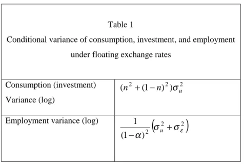
Conditional Variances
Table 1 documents the conditional (on the current capital stock) variance of consumption, investment, and employment, in the economy with floating exchange rates. Consumption variance is less than employment variance. In addition, consumption variance is independent of the variance of technology shocks.
Table 1
Conditional variance of consumption, investment, and employment under floating exchange rates
Consumption (investment) Variance (log) 2 2 2
)
)
1
(
(
n
+
−
n
σ
uEmployment variance (log)
(
2 2)
2)
1
(
1
εσ
σ
α
+
−
u Price DeterminationThe solution for consumption, investment, and employment takes as given the pre-set prices
P
ht,P
ft. But these prices must be determined optimally, ex ante, using condition (14). Recognizing that consumption and investment are in proportion to one another allows this condition to be significantly simplified. We get)
))
(
1
(
)
(
(
)
1
)(
1
(
)
~
1
(
1 1 1 − − −−
−
−
−
=
t ht t t t hP
z
H
z
H
E
P
α
λ
λ
βα
λη
.Substituting for the definition of employment from (27) gives
(28)
−
−
−
−
=
− − − − − − − α α ρ α α ρε
θ
ϕ
ε
θ
ϕ
α
λ
λ
βα
λη
1 1 1 1 1 1 1 1 1)
exp(
)
exp(
1
)
exp(
)
exp(
)
1
)(
1
(
)
~
1
(
1
ht t t t t t ht t t t t t tP
K
u
M
P
K
u
M
E
,where
)
~
1
(
)
1
(
λ
βα
βµ
ϕ
=
−
−
. Examining (28), it is clear that the equilibrium pre-set priceht
P
will be proportional to
− − α ρθ
ϕ
t t tK
M
11 , which is already in the period t-1 information set. We
may thus characterize the solution for
P
ht as(29)
Θ
=
− − α ρθ
ϕ
t t t htK
M
P
1 1 ,where Θsatisfies the following condition
(30)
Θ
−
−
Θ
−
−
−
−
=
− − − α αε
ε
α
λ
λ
βα
λη
1 1 1 1 1)
exp(
1
)
exp(
)
1
)(
1
(
)
~
1
(
1
t t t t tu
u
E
,If
σ
t2=
σ
ε2=
0
, thenΘ
=
( )
H
−(1−α) would hold. Thus, (30) implicitly describes also the determination of expected employment in the home country. In general however, the value ofΘis going to depend on the distribution of
exp(
u
t−
ε
t)
. Figure 1 illustrates how equation (30) determines)
)
1
(
(
1 t t tH
H
E
−−
. Since this is a convex function ofH
t, an increase in the variance ofH
t must reduceE
t−1(
H
t)
, in order to keep)
)
1
(
(
1 t t tH
H
E
−−
constant. The model therefore implies that there is a negative relationship between the variance of employment, and the mean employment level.The intuitive explanation of this relationship is that a rise in the variability of
employment, generated either by monetary shocks or technology shocks, will increase expected marginal costs facing firms. This will lead them to set higher prices, conditional on the predicted values of money, technology, and the capital stock. Thus, an increase in the variance of
exp(
u
t−
ε
t)
will raise Θ. An increase in the mean price level will reduce the mean value of employment implied by equation (27).The value of employment and the pre-set price level for the foreign economy can likewise be calculated, using identical procedures. We reach the same conclusions; foreign money and technology uncertainty biases down the mean level of employment9.
Dynamics
Now using the solution for prices, we may describe the full dynamic path of
consumption, the capital stock, and output in each country. Substituting (29) into the equation for investment, (26), we obtain
(31)
βα
λ
θ
ρθ
ρ αt n t n t t t tnu
n
u
K
K
Θ
−
=
− − − +1
)
)
1
exp((
)
exp(
~
*(1 ) 1 1 * 1 .Investment is affected by technology shocks only with a one period delay. Within any period, a technological improvement has no impact on consumption, investment, or output. But prices are adjusted after one period. A persistent technology shock, for instance in the home country, will lead to a fall in home country prices in the next period, which allows for an increase in
consumption and investment for both countries. The rise in foreign consumption is achieved through a terms of trade deterioration for the home economy.
Since (31) depends upon Θ, it follows that the unconditional mean of the capital stock, consumption, and output are also affected by the volatility of money and technology10. The unconditional mean level of
ln
K
is given by:(
ln(
~
)
ln(
)
)
)
1
/(
1
−
−
Θ
=
α
βα
λ
k
.This is also negatively related to the volatility of money and technology shocks. The same holds true for consumption and output.
Also from (31), we may derive the unconditional variance of (the log of) consumption and investment and real GDP in the home (and foreign) economy. It is written as
(
)
2 2 2 2 2 2 2 2 2 2 2)
1
(
)
1
(
1
)
1
(
)
1
(
1
1
εσ
ρ
ρ
α
α
αρ
ρ
σ
α
−
+
−
+
−
+
−
+
−
n
n
u . 9The relationship between the volatility and mean of macroeconomic aggregates has been shown in a different context by Devereux and Engel (1998).
10
The absolute level of the capital stock is influenced by volatility in two ways. First, a higher volatility of (for instance) domestic money raises the expectation of
exp(
nu
t)
, which increases the capital stock. But in addition, a higher volatility of money raised Θ, which reduces the capital stock. The net result of monetary volatility on the level ofK
t+1 is ambiguous.Real GDP variance depends upon the variance of both money shocks and technology shocks. Note that the smaller is the persistence in technology shocks (i.e. the smaller is
ρ
), the smaller is the influence of technology shocks on output variance. If technology shocks were entirely transitory (ρ
=0), output variance would be unaffected by technology shocks at all. This makes sense, since if there is no persistence in the technology shock, there is no ex post readjustment of prices to reflect the shock.The unconditional variance of employment is in fact the same as the unconditional variance in Table 1. This is because employment is unaffected by anticipated movements in the capital stock and in technology.
Section 5: Fixed exchange rates
Since prices are pre-set, it would seem that the exchange rate regime would have a significant effect on allocations and welfare in this economy. More generally, following the discussion of the introduction, we will investigate whether the decision to fix exchange rates involves a sacrifice due to the inability of relative prices to adjust in response to supply shocks.
One important issue to confront is just how the exchange rate is fixed. Any set of monetary policies that keeps the exchange rate constant is consistent with a fixed exchange rate. In the floating exchange rate environment described above, we assumed that the home and foreign country had independent randomness in their money supplies, so that exchange rates would in general fluctuate. We have assumed that in order to fix exchange rates the monetary authorities sets money supplies the same across countries. But there are many different ways to do this. One assumption is that the money supply process in each country follows a country weighted average of the money supply processes in a floating exchange rate regime. That is (32)
M
t=
M
t*=
M
t−1exp(
nu
t+
(
1
−
n
)
u
t*)
.This keeps the exchange rate constant and always equal to unity. Moreover, it maintains the variance of the world money supply equal to the variance of a country weighted average of money supplies in the floating exchange rate regime. But the variance of the (log) money supply within each country is actually smaller than under floating. This represents what might be called a `cooperative peg' exchange rate regime.
An alternative assumption is that the one country adjusts its money supply to follow the policy of the other country, so as to maintain the pegged rate. If we took the foreign country as the follower, then this would entail that it set its money supply equal to that of the home country, so that
(33)
M
t*=
M
t=
M
t−1exp(
u
t)
.This might be called a `one-sided peg' exchange rate regime. It implies that the variance of the money supply in each country is the same as under floating (since the monetary shocks had been assumed to have equal variance to begin with). But the variance of world money supply exceeds that of the country weighted average of money supplies under floating exchange rates.
The implications of a fixed exchange rate regime are obtained by simply imposing either the monetary rule (32) or (33) on to the solutions for consumption, investment and employment from (25)-(27). Table 2 illustrates the implications for the conditional variance of consumption, investment and employment, for the cooperative peg regime. Table 3 shows the same variables in the case of the one-sided peg.
A number of conclusions can be drawn from the Tables. First, in the cooperative peg, the conditional variance of consumption and investment is unaffected by the fixed exchange rate. It is easy to see why from (25). Whether the exchange rate is fixed or floats, consumption is determined by a geometric average of national money stocks. But in the cooperative peg, each countries money stock is a geometric average of the money stocks under floating exchange rates. Thus consumption (and investment) volatility is identical under the two regimes. On the other hand, since each individual country's money supply variance falls, the conditional variance of employment also falls. Therefore, while consumption and investment volatility remains unchanged, employment volatility falls11.
For the one-sided peg regime, the situation is exactly the reverse. Because the variance of the world money supply is higher, consumption and investment volatility is higher in a fixed exchange rate regime. But employment volatility is unchanged, since the volatility of each individual national money supply is not changed by the move to fixed exchange rates (given our assumption of identical money variances).
11
Employment is determined by total demand (consumption and investment) and relative prices (the terms of trade). A fixed exchange rate leaves demand volatility unchanged, but reduces terms of trade volatility, and so reduces employment volatility.
Table 2
Conditional variance, consumption, investment and employment under fixed exchange rates (cooperative peg)
Consumption (investment) Variance (log) 2 2 2
)
)
1
(
(
n
+
−
n
σ
uEmployment variance (log)
(
2 2 2 2)
2(
(
1
)
)
)
1
(
1
εσ
σ
α
+
−
+
−
n
n
u Table 3Conditional variance, consumption, investment and employment under fixed exchange rates (one-sided peg)
Consumption (investment) Variance (log)
2
u
σ
Employment variance (log)
(
2 2)
2)
1
(
1
εσ
σ
α
+
−
uThe exchange rate regime will also make a difference for the average level of prices. In the cooperative peg regime, the coefficient Θ is determined by the condition:
(34)
Θ
−
−
+
−
Θ
−
−
+
−
−
−
=
− − − α αε
ε
α
λ
βα
λη
1 1 * 1 1 * 1)
)
1
(
exp(
1
)
)
1
(
exp(
)
1
)(
1
(
)
1
(
1
t t t t t t tu
n
nu
u
n
nu
E
.Given that money and supply shocks are independent, it is clear that the value of
Θimplied by (34) is lower than that under floating exchange rates. Therefore, average prices are lower in both countries in a cooperative peg. By implication, average employment is higher. For the one-sided peg, the condition determining average prices is the same as (30). Since the variance of money for each country is unchanged, it follows that the value of Θis unchanged.
Therefore, the fixed exchange rate under a one-sided peg has no implications for prices, and average employment is the same as under a floating regime.
In the cooperative peg, the dynamic process for the capital stock is identical to (31), except for the fact that the Θterm is lower. In the one-sided peg, the capital stock process is
(35)
βα
λ
θ
ρθ
ρ tα n t n t t tu
K
K
Θ
=
− − − +1
)
exp(
~
*(1 ) 1 1 1 .where Θ is the same as under floating exchange rates.
Using (35), following the logic of the previous section, it can be seen that the unconditional mean of (log) consumption, the capital stock, and real GDP are higher in a
cooperative peg than under an floating regime. Therefore, moving from a floating exchange rate to a fixed exchange rate under a cooperative peg actually increases average GDP.
An important implication of these results is that the response of the economy to technology shocks is independent of the exchange rate regime. The conditional volatility of consumption and investment does not depend on technology variance. While the conditional variance of employment does depend on technology variance, the component of employment volatility that is explained by technology variance is independent of the exchange rate regime. Intuitively, with pre-set prices, consumption, investment and output are determined solely by aggregate demand shocks. Within the period within which prices are set, technology shocks only impact on employment. This means that the exchange rate regime cannot help in any way to improve the economy's adjustment to technology shocks. Even in the face of country specific technology shocks that in the flexible price environment would require terms of trade adjustment (according to (20)), floating exchange rates do not function to provide this adjustment potential. In the absence of monetary shocks, there is in fact no difference at all between the economy with floating exchange rates and fixed exchange rates.
More generally, it can be seen from (35) that the role of technology shocks in the unconditional volatility of real GDP is independent of whether the exchange rate is fixed or floating. Technology shocks affect output, consumption and investment only with a one period lag. But this property holds across all different exchange rate regimes.
Section 6. Welfare and exchange rate regimes
We may conduct a welfare comparison of the floating exchange rate regime with the two types of fixed exchange rate regimes. Welfare may be defined as the expected utility of the
representative individual (in either country). Define the value function for an individual as as function of initial capital and the technology shocks from one period ago12;
)
,
(
−1 *−1=
V
K
t t tV
θ
θ
Given the structure of the model, it is not surprising that we can solve for the exact form of the value function. It is given by
(36)
V
=
A
+
B
ln
K
t+
D
1ln(
θ
t−1)
+
D
2ln(
θ
t*−1)
, whereA
,B
,D
1 andD
2are constants, given byΘ
−
+
−
−
+
Ω
=
−ln
1
1
)
1
ln(
1 0βα
χ
η
E
tH
tA
,βα
α
χ
−
+
=
1
)
1
(
B
,)
1
)(
1
(
)
1
(
1βρ
βα
ρ
χ
−
−
+
=
n
D
,)
1
)(
1
(
)
1
(
)
1
(
2βρ
βα
ρ
χ
−
−
−
+
=
n
D
.Given the structure of the economy, the exchange rate regime affects only the constant term A in
the value function. Recall by (27) and (29),
ε
−α
Θ
−
=
1 1)
exp(
t t tu
H
.An important feature of (36) is that it does not involve the markup term
λ
~
. The markup pricing rule (14) involves a distortion which biases down average employment. A social planner would choose Θso that equilibrium employment would be given by)
1
(
)
1
)(
1
(
)
1
)(
1
(
ˆ
βα
η
α
χ
α
χ
−
+
−
+
−
+
=
H
.This always exceeds
H
, the flexible price equilibrium employment level. The planner would like too eliminate the effects of the markup on employment. In addition, the planner would take into account the affect of employment on equilibrium real money balances 13.
12 In the presence of the constraint on ex ante price setting, it is natural to define welfare as a function of
state variables in the date t-1 information set. In addition, the value function does not depend on the money stock since the anticipated value of the money stock has no effect on welfare.
13
This second inefficiency is due to the fact that the presence of a positive nominal interest rate implies a deviation from the Friedman rule in monetary policy. Higher employment would increase consumption and real balances, moving the economy closer to the Friedman rule. Under our specification, however, the Friedman rule (or zero nominal interest rate) would imply an infinite level of real money balances.