HAL Id: pastel-00913469
https://pastel.archives-ouvertes.fr/pastel-00913469
Submitted on 3 Dec 2013
HAL is a multi-disciplinary open access archive for the deposit and dissemination of sci-entific research documents, whether they are pub-lished or not. The documents may come from teaching and research institutions in France or abroad, or from public or private research centers.
L’archive ouverte pluridisciplinaire HAL, est destinée au dépôt et à la diffusion de documents scientifiques de niveau recherche, publiés ou non, émanant des établissements d’enseignement et de recherche français ou étrangers, des laboratoires publics ou privés.
Programmation sûre en précision finie : Contrôler les
erreurs et les fuites d’informations
Ivan Gazeau
To cite this version:
Ivan Gazeau. Programmation sûre en précision finie : Contrôler les erreurs et les fuites d’informations. Analyse numérique [cs.NA]. Ecole Polytechnique X, 2013. Français. �pastel-00913469�
Safe Programming in Finite Precision:
Controlling Errors and Information Leaks
Thèse de Doctorat
Spécialité informatique
présentée et soutenue publiquement le 14 octobre 2013 par
I
VANG
AZEAUDevant le jury composé de :
Directeurs de thèse : Dale Miller (INRIA, École Polytechnique) Catuscia Palamidessi (INRIA, École Polytechnique)
Rapporteurs : Michele Boreale (University of Florence, Italy)
Herbert Wiklicky (Imperial College, UK)
Examinateurs : Eric Goubault (CEA)
Olivier Boissou (CEA)
A
CKNOWLEDGMENTS
I would like to thanks Dale for his support all along my PhD. He has been a great advisor who provides me insights about where to find deep material. He was always available to hear about my progress and new investigations and support me to burry on my ideas. I also would like to thanks Catuscia for her investment in my PhD. She provide me very good insights as weel as she has been very pedagogic with me, especially about the way to introduce and to present my work. The topics adressed during my PhD were quite broad, so I really appreaciate the complementarity of the expertise of Dale and Catuscia that allow me to get a large perspective.
I am honoured that Herbert Wicklicky and Michele Boreales have accepted to review my thesis and I thank them for their careful reading.
I am delighted that Olivier Buissou and Eric Goubault accepted to be part of my jury. This thesis was partly founded by the ANR project Confidence Proof and Provability, where I had the pleasure to meet Olivier Buissou who was a charismatic organisor and Eric Goubault who spends a lot of time to introduce me to the present challenges of finite-precision arithmetics .
I also thanks Jean Goubault-Larrecq that was co-organizer of the ANR project for his advices and expertize on my research project. I worked for a while with Filippo Bonchi, even if at the end, we did not concretize our work, I have been very pleased to exchange ideas with him.
Because scientific work is not possible without a warm and convivial environment, I would like to thanks all former and later members of the Parsifal and the Comete team. I have a special thought for my parents and family that encourage me all along my PhD, I also warmly thanks my roomates Cyrille, Gilles and Olivier for the nice three years of life together and I lovely thanks Isabelle for everything.
Finally, I would like to thank you, dear reader, for your attention on my thesis work.
C
ONTENTS
Résumé en français v
0.1 Robustesse . . . vi
0.2 Confidentialité différentielle . . . viii
0.3 Analyse globale d’un programme . . . x
1 Introduction 1 1.1 Contributions and plan of the thesis . . . 3
1.2 Publications . . . 4
2 Robustness 5 2.1 Hardware and semantics preliminaries . . . 6
2.1.1 The fixed-point representation . . . 6
2.1.2 The floating-point representation . . . 7
2.1.3 Semantics of programs. Definitions and notations . . . 9
2.1.4 Problems induced by the rounding error . . . 10
2.2 Quantitative analysis . . . 12
2.2.1 Static analysis . . . 13
2.2.2 Input-output relation . . . 14
2.2.3 Dealing with several variables . . . 15
2.2.4 Internal rounding error . . . 18
2.3 Our approach to robustness . . . 19
2.3.1 Input-output relation . . . 19
2.3.2 Robustness with respect to the exact semantics . . . 22
2.4 Conclusion . . . 25
3 Differential Privacy 26 3.1 Introduction . . . 26
3.1.1 Related work . . . 30 ii
3.1.2 Plan of the chapter . . . 31
3.2 Preliminaries and notation . . . 31
3.2.1 Geometrical notations . . . 31
3.2.2 Measure theory . . . 33
3.2.3 Probability theory . . . 34
3.3 Differential privacy . . . 35
3.3.1 Context and vocabulary . . . 35
3.3.2 Previous approaches to the privacy problem . . . 36
3.3.3 Definition of differential privacy . . . 38
3.3.4 Some properties of differential privacy . . . 39
3.3.5 Standard technique to implement differential privacy . . . 40
3.4 Error due to the implementation of the noise . . . 41
3.4.1 The problem of the approximate computation of the true answer . . . . 42
3.4.2 General method to implement real valued random variables . . . 43
3.4.3 Errors due to the initial random generator . . . 45
3.4.4 Errors due to the function transforming the noise . . . 48
3.4.5 Truncating the result . . . 51
3.4.6 Modeling the error : a distance between distributions . . . 53
3.4.7 Rounding the answer . . . 56
3.4.8 Strengthening the differential privacy property . . . 58
3.5 Preserving differential privacy . . . 62
3.6 Application of the Laplacian noise in one dimension . . . 64
3.6.1 Requirements and architecture assumptions . . . 64
3.6.2 Weakness of the mechanism . . . 65
3.6.3 Improvement of the implementation . . . 67
3.7 Application to the Laplacian noise in two dimensions . . . 69
3.8 Conclusion and future work . . . 72
3.8.1 Conclusion . . . 72
3.8.2 Future work . . . 72
4 Global analysis of programs 74 4.1 Presentation of the problem . . . 76
4.1.1 Cordic . . . 77
4.1.2 Dijkstra’s shortest path algorithm . . . 82
4.2 Semantic pattern matching . . . 85 4.3 A direct analysis of the finite precision semantics through program transformation 87
4.3.1 The schema structure . . . 87
4.3.2 A sufficient condition for robustness . . . 88
4.3.3 Application to the CORDIC algorithm . . . 91
4.3.4 Application to the Dijkstra’s shortest path algorithm . . . 97
4.3.5 Discussion . . . 103
4.4 Analysis through rewriting techniques . . . 103
4.4.1 Preliminaries: the rewriting framework . . . 104
4.4.2 Application of the rewriting framework . . . 105
4.4.3 Sufficient conditions to prove the closeness property . . . 108
4.4.4 Application to the CORDIC algorithm . . . 112
4.4.5 Application to Dijkstra’s algorithm . . . 118
4.4.6 Approximate confluence . . . 122
4.5 Conclusion . . . 127
R
ÉSUMÉ EN FRANÇAIS
Contrairement à l’homme qui manipule des valeurs symboliques lors de ses calculs (√2, π, etc.), un ordinateur calcule à partir d’approximation des nombres. En effet, même s’il est possible, de nos jours, d’implémenter le calcul symbolique, celui-ci reste coûteux en ressources et est beaucoup plus lent qu’un calcul direct à base d’approximations. Bien entendu, le fait d’arrondir les nombres provoque des erreurs de calculs, et même si tout est fait au niveau de l’architecture des processeurs pour rendre ces erreurs aussi négligeables que possible, celles-ci peuvent, dans certaines circonstances, perturber fortement le résultat.
Ces erreurs d’arrondis dont certaines sont restées tristement célèbres (explosion de la fusée Ariane 5, explosion d’un missile sur une mauvaise cible) ont toujours été et font toujours l’objet d’études approfondies. Comme les preuves manuelles de correction ont toujours le risque d’être fausses et requerraient trop de travail pour des logiciels industriels comportant des milliers de lignes de code, on a développé des programmes pour automatiser l’analyse des programmes.
L’analyse de programmes est appelée statique car le programme n’est pas exécuté, contraire-ment aux analyses à base de tests. Cela lui permet de fournir une garantie totale de la robustesse du programmes aux erreurs (contrairement aux tests qui, généralement, ne sont pas exhaustifs et sont donc faillibles). Dans cette thèse cependant, nous ne cherchons pas à développer une méthode d’analyse automatique ou semi-automatique mais nous cherchons à relier des preuves de corrections d’algorithmes à des analyses automatiques de code. En effet, dès que le principe d’un programme est non trivial, il repose souvent sur un théorème qui prouve que l’algorithme va fournir le bon résultat. Ce théorème peut potentiellement utiliser des arguments mathéma-tiques complexes et sera donc la plupart du temps hors d’atteinte d’un analyseur automatique. Mais malheureusement, les théorèmes sont souvent prouvés uniquement pour un calcul exact et ne permettent pas de prédire quantitativement l’influence des erreurs d’arrondis lors du calcul. Le but de cette thèse est de proposer pour deux classes d’algorithmes des théorèmes étendus qui, en se basant sur la preuve exacte et sur une analyse simple du code, permettent de quantifier l’erreur finale résultant des arrondis.
Les deux problèmes que nous avons abordés sont les suivants. D’abord nous nous sommes intéressé à la question de la confidentialité différentielle (differential privacy). Il s’agit d’un
vi 0.1
mécanisme permettant à un individu de participer à une étude statistique sans que l’on puisse retrouver ses données personnelles. L’intérêt de ce problème est que le programme ne calcule pas la valeur d’une fonction mais produit une valeur (pseudo)-aléatoire. Or, comme un analyseur automatique ne fournit qu’une borne sur la déviation maximale d’un calcul, il faut réussir à réinterpréter cette déviation en terme de variation de la loi de probabilité.
Dans notre second problème, on s’intéresse à des programmes où les branchements condi-tionnels modifient radicalement la façon dont on atteint le résultat. Dans de tels programmes, une infime variation dans les valeurs peut conduire le programme à emprunter deux branches dont les effets sont radicalement différents. Bien sûr, de tels programmes fonctionnent car, au final, il y a une sorte de convergence qui s’opère. Cependant, un analyseur fait progresser son analyse ligne après ligne par compositions successives et ne peut pas appréhender cette conver-gence globale. De fait, quand il se retrouve face à deux branches distinctes qui mènent à des résultats différents, il risque de simplement conclure que le programme est instable. Pour palier à ce problème nous proposons un théorème qui utilise la propriété de convergence prouvée pour des calculs exacts ainsi qu’une analyse du programme qui ne se soucie pas des branchements pour conclure un résultat de robustesse pour le programme en calcul arrondis.
0.1
Robustesse
Représentation finie
Avant de prouver la fiabilité d’un programme, il est important de comprendre en quoi consiste exactement le calcul en représentation finie. Principalement, nous nous intéressons à deux types de représentations finies : les nombres à virgules flottantes et les nombres à virgules fixes.
Les nombres à virgules fixes sont utilisés soit sur des processeurs rudimentaires soit pour des calculs où l’amplitude des nombres est connue à l’avance (la monnaie par exemple) soit dans quelques cas où ils sont plus performants que les nombres à virgule flottante. Leur représen-tation consistent principalement en un entier divisé par une constante prédéfinie. Lors d’un calcul en virgule fixe, les additions et soustractions se font sans erreur car le résultat est aussi représentable. Le principal problème de cette représentation, c’est qu’elle ne permet pas de représenter de très grand nombres donc une multiplication peut facilement déclencher un dé-passement de capacité.
Les nombres à virgules flottantes sont plus élaborées car ils possèdent un exposant variable et non constant (d’où le nom de flottant). Ces nombres étant les plus utilisés, leur comportement est strictement encadrée par le standard IEEE 754. Les opérations primitives (addition, soustraction, multiplication, division, logarithme, exponentielle, passage à l’exposant) sont garantis pour avoir
0.1 Robustesse vii
un résultat avec une précision totale: le résultat (arrondi) est tel qu’il n’existe aucun autre nombre représentable entre lui et le résultat exact. En d’autres termes, l’erreur vient juste de l’arrondi, il n’y a pas d’erreur de calcul. Cependant, cette propriété n’est vraie que pour une opération. Dès qu’un programme va enchaîner un nouveau calcul sur une opération déjà arrondie, l’arrondi final ne sera pas forcément optimal.
Analyse statique
Le but de cette thèse est de proposer des outils qui viennent en aval d’une première analyse statique du code, aussi, nous décrivons brièvement leur principe de fonctionnement ainsi que les enjeux de ces analyses.
Il y a deux familles de méthodes généralement utilisées. D’une part il y a les preuves logiques basées sur les triplets de Hoare. Cette méthode reprend les techniques utilisées pour prouver les formules logiques. Un triplet de Hoare consiste en une précondition, un élément de syntaxe du code à étudier et une postcondition. L’autre famille d’analyseur est basée sur l’interprétation abstraite. Dans ce cas, on définit à l’avance un domaine abstrait qui, en re-groupant plusieurs états de la mémoire en un seul, permet de prédire des propriétés du résultat pour n’importe quel entrée.
Indépendamment de la méthode employée, il faut définir ce qu’on entend par robustesse. La première définition est une relation entre l’entrée et la sortie. On souhaite que de petites perturbations de l’entrée n’aient pas d’impact majeur sur la sortie du programme. Dans le cas contraire, une erreur de mesure ou une erreur provenant d’un calcul précédent générerait une erreur arbitraire indépendamment de la précision du programme lui-même.
La deuxième propriété à considérer est celle de l’erreur interne causée par le programme. Tandis que la question de l’entrée / sortie est inhérente à la fonction qu’on calcule, l’erreur interne se définit entre la sémantique exacte du programme et sa sémantique effective avec erreur. Enfin, nous soulevons la question de la gestion de plusieurs variables. Comme nous souhaitons une modélisation la plus souple possible, nous introduisons la notion de mesure qui permet de gérer de façon simple et uniforme un ensemble arbitraire de variables.
Notre approche
A partir de ces analyses sur ce qu’est un nombre en représentation finie et ce que fait une analyse statique de programme, nous justifions deux définitions de la robustesse que nous utiliserons par la suite. En effet, la plupart des propriétés que fournit un analyseur automatique permettent de déduire les propriétés que nous proposons. De plus, celles-ci sont simples à manipuler mathé-matiquement et permettent ainsi de se combiner facilement aux preuves du programme dans la
viii 0.2
sémantique exacte. La première des deux définitions, la propriété P(k,ε), concerne uniquement la question des entrées/sorties. Tandis que la seconde, la propriété de (k,ε)-promixité, concerne l’écart entre la sémantique exacte et la sémantique effective.
0.2
Confidentialité différentielle
L’analyse statique permet, dans son usage le plus fréquent, de mesurer l’erreur induite par le pro-gramme et permet, par exemple, d’informer l’utilisateur du propro-gramme du nombre de décimales qui ne sont pas affectées par ces erreurs. Dans le chapitre 3, nous nous intéressons aux problèmes de l’erreur dans un contexte différent. Ici, il s’agit de comprendre l’impact des erreurs de calculs pour un programme utilisé dans la protection des données. Précisément, on peut vouloir fournir un résultat à partir de données qui doivent rester confidentielles. Dans ce cas, le problème n’est pas vraiment que le résultat soit imprécis mais, avant tout, qu’une corrélation entre la nature de l’erreur et les entrées peut permettre à celui qui reçoit le résultat d’obtenir des informations sur les entrées confidentielles. Dans le cas qui nous intéresse, la confidentialité différentielle, nous montrons que son implémentation stricte, telle que spécifiée théoriquement pour un calcul exact, va provoquer des failles importantes. Il est donc nécessaire d’adapter l’implémentation pour empêcher ces failles. Ensuite, il s’agit de montrer que le nouveau protocole est sûr malgré les erreurs de calcul. Plus précisément, il s’agit de mesurer la perte provoquée par les erreurs d’arrondis et de montrer que celle-ci est acceptable. Après avoir montré brièvement le type de faille qui peuvent apparaître, l’essentiel de ce chapitre se concentre sur une modélisation du problème qui soit la plus indépendante possible de la représentation finie utilisée ainsi que du programme lui-même (on suppose juste qu’il répond aux spécifications sans présupposer du code lui-même). A partir de cette modélisation, nous établissons, via un théorème, la perte en confidentialité induite par les erreurs. Enfin, nous montrons deux applications possibles de ce théorème suivant le type de données à protéger.
Description de la confidentialité différentielle
La confidentialité différentielle est une approche ayant pour but de garantir la confidentialité des données des participants à une étude statistique. En effet, une base de donnée à usage statistique doit révéler des informations générales sur les participants telles que des moyennes ou l’existence de certaines corrélations. Cependant, la plupart des participants à ses bases de données n’acceptent de livrer leur données que si on leur promet que leurs informations person-nelles ne seront pas divulguées. Ainsi, il faut pouvoir, par exemple, être en mesure de donner le pourcentage de la population qui fume sans révéler qui, précisément, fume.
0.2 Confidentialité différentielle ix
Pour satisfaire ces deux contraintes, la protection de la vie privée et la publication d’infor-mations générales, de nombreuses méthodes ont été proposées. La première a été de se contenter d’anonymiser les identifiants personnels des participants puis de transmettre les données ainsi anonymisées aux analystes qui sont alors libres de faire les requêtes qu’ils souhaitent. Une telle méthode ne permet cependant pas de garantir l’anonymat: rien ne garantit en effet qu’un analyste ne possède pas déjà une partie des informations de la base de donnée. Par exemple, dans une base médicale, même si on supprime les nom, prénom et numéro de sécurité sociale des participants, on conservera leur âge selon toute vraisemblance. Supposons maintenant que la doyenne des français participe à l’étude. Étant probablement la seule de son âge, il est facile pour un analyste de trouver à quelle entrée elle correspond et de connaître ainsi tout son dossier médical. On peut chercher, par exemple, la proportion de diabétiques parmi les personnes de plus de 112 ans.
Ce type d’attaque peut sembler simple à prévenir, aussi d’autres méthodes d’anonymisation ont vu le jour pour parer au problème. Cependant, par des attaques plus complexes ces autres méthodes se sont elles aussi avérées vulnérables. La confidentialité différentielle repose sur un protocole plus strict que ses prédécesseurs : aucune partie de la base de données n’est jamais fournit à l’analyste. Au lieu de cela, l’analyste doit, pour chaque requête, contacter la base de données qui est détenue par un agent de confiance. Celui-ci répond aux requêtes de façon prob-abiliste en ajoutant de l’aléatoire dans sa réponse. La propriété de confidentialité différentielle stipule que la probabilité d’obtenir une réponse donnée à une requête est sensiblement la même qu’une personne donnée participe ou non à la base de donnée. Autrement dit, on ne risque rien à participer à la base de donnée puisque si on ne participait pas, les analystes obtiendraient des réponses qui seraient indiscernables à celles obtenues en cas de participation.
Pour obtenir cette propriété, il faut que le facteur aléatoire soit proportionnel à la sensibilité de la requête à la présence d’un individu supplémentaire quelconque. De la sorte, si une requête cible trop précisément un individu, le bruit ajouté sera suffisamment important pour masquer l’information.
L’implémentation théorique et ses faiblesses en pratique
Pour obtenir cette propriété, la méthode théorique consiste à calculer le résultat réel de la re-quête puis d’ajouter une valeur aléatoire répartie selon une distribution adéquate (par exemple la distribution de Laplace) dont l’amplitude dépendra du degré de confidentialité recherché et de la sensibilité de la requête.
Cette méthode fonctionne en théorie mais elle s’appuie sur le fait qu’il existe des proba-bilités de distribution continue (deux valeurs proches ont des probaproba-bilités quasiment identiques
x 0.3
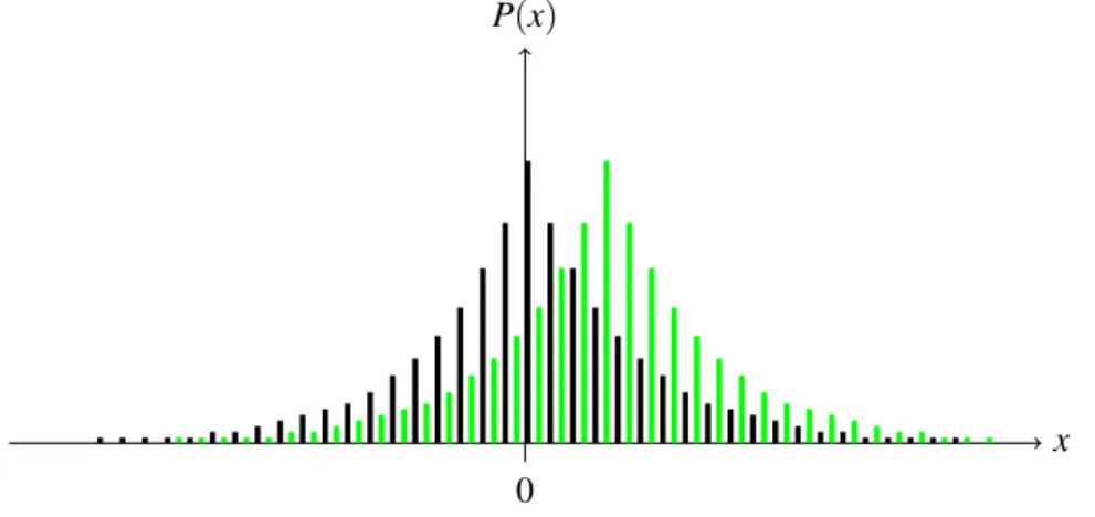
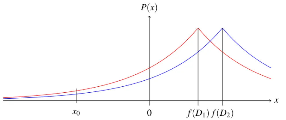
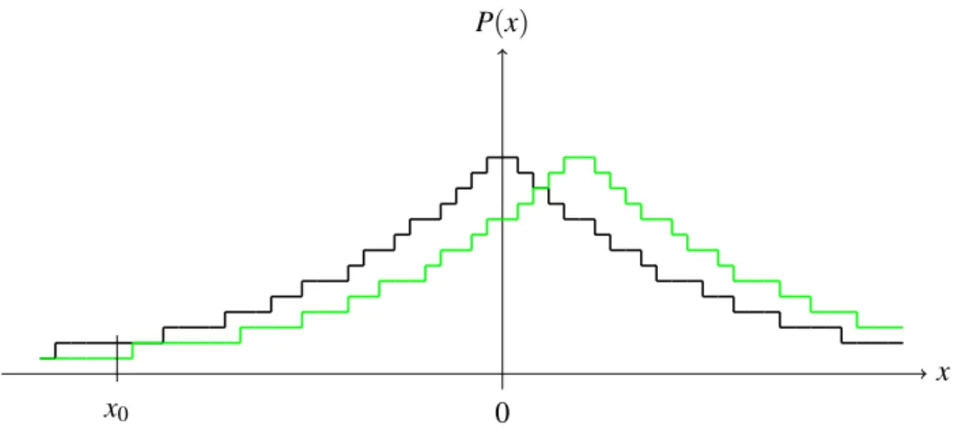
d’apparaître). Elle repose également sur le fait qu’il est possible qu’une variable aléatoire puisse produire des valeurs arbitrairement grandes avec une probabilité arbitrairement faible. Or ces deux propriétés ne sont plus conservées lorsqu’on génère une valeur pseudo-aléatoire en pré-cision finie. En effet, à cause des arrondis (et, a fortiori, en cas d’erreur de calcul) certaines valeurs précisent peuvent ne pas être représentée du tout tandis qu’une valeur proche peut appa-raître avec une probabilité plus élevée qu’elle ne devrait (voir figure 3.1). De cette façon, il n’y a plus de continuité dans la distribution de la probabilité. Nous montrons dans l’exemple 3.1.1 comment ce défaut permet d’accéder à des informations confidentielles.
Modélisation et analyse de la situation en précision finie
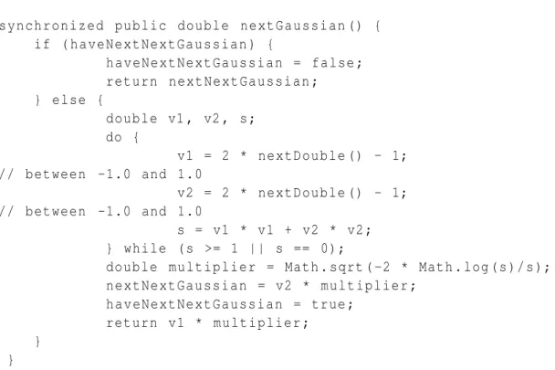
Dans la partie technique du chapitre 3, nous montrons d’abord comment sont générées les vari-ables pseudo-aléatoires. Nous montrons que celles-ci peuvent être assimilées à des varivari-ables aléatoires parfaites qui ont subit une perturbation (non contrôlée celles-ci) d’amplitude bornée.
Ensuite nous proposons une amélioration du protocole qui va palier aux défauts décrits précédemment: pour éviter les irrégularités locales de la distribution, on impose que le résultat retourné soit arrondi plus que la précision de la machine. Pour palier au fait qu’une représenta-tion finie ne peut produire des nombres arbitrairement grands avec une probabilité arbitrairement faible, on impose de retourner une erreur si le résultat produit dépassait une certaine borne. En-fin, on traduit la déviation en terme de distance entre distributions de probabilité. Après avoir rajouté une dernière contrainte quant à la forme de la distribution utilisée, on prouve que la perte de confidentialité est bornée par une constante calculable.
On montre ensuite comment le théorème s’applique dans le cas standard le plus simple. On montre que dans certains cas, malgré les contraintes supplémentaires, la perte peut demeurer importante. On propose alors une autre façon de générer les nombres pseudo aléatoire pour ce cas qui réduit drastiquement cette perte. Enfin on montre que notre analyse permet aussi de traiter des données plus complexes comme des bases de données ayant des données à valeur dans le plan euclidien.
0.3
Analyse globale d’un programme
Dans le chapitre 4, nous nous intéressons à l’analyse du programme elle-même, à savoir borner l’erreur provoquée par la représentation finie d’un programme donné. Comme nous l’avons précédemment évoqué, il existe déjà plusieurs façon d’analyser automatiquement un code donné. Cependant ces méthodes fonctionnent de façon progressives. En quelque sorte, elles extraient une information sur cette borne pour les n premières lignes du code à partir de laquelle elles
0.3 Analyse globale d’un programme xi
fournissent une information sur les n + 1 lignes de code. Et ainsi de suite jusqu’à atteindre la fin du programme.
Ici on s’intéresse à des programmes qui ne peuvent pas être analysés de cette façon. En effet, certains programmes produisent une erreur importante en cours d’exécution qui ne se résorbe qu’à la fin de l’exécution. C’est le cas par exemple des programmes qui effectuent une dichotomie pour trouver une valeur : au moment où on teste si la valeur cherchée est supérieure ou inférieure, une erreur de calcul peut mener dans l’autre branche du test. Dans ce cas, le programmes va poursuivre avec des valeurs très différentes de celles qu’il aurait dû prendre mais la valeur finale va tout de même s’approcher de la valeur exacte. Pour illustrer notre analyse sur ce type de phénomène, on a pris comme exemple l’algorithme CORDIC qui calcule la fonction sinus. Un autre cas est celui où l’ordre dans lequel on effectue une tâche permet un certain parallélisme: à cause des erreurs de calcul, on peut choisir de commencer par une tâche plutôt que par une autre (et donc avoir un état intermédiaire très différent de l’état théorique) mais, à la fin, une fois les deux tâches effectuées le résultat est quasiment identique. Pour illustrer cet autre type de phénomène, nous avons choisi d’étudier l’algorithme de Dijkstra qui calcule le plus court chemin dans un graphe.
La méthode d’analyse que nous proposons utilise la preuve mathématique qu’un algorithme est correct pour borner l’erreur que peut générer son implémentation en représentation finie. Par exemple, dans le cas de CORDIC, on va utiliser le fait qu’avec des calculs exacts l’algorithme produit une fonction continue de dérivée bornée (pour le calcul de la fonction sinus). Cependant cette propriété ne peut pas être exploitée directement car la preuve part du principe, entre autres, que des rotations d’un point autour d’un même axe vont conserver la distance de ce point à l’axe. Cela ne sera plus le cas dans l’implémentation: les erreurs de calculs pourront aussi translater ce point et l’éloigner ou le rapprocher de l’axe.
En plus de cette preuve en sémantique exacte, nous décomposons le programme selon un motif prédéfini qui va nous permettre, d’une part, d’analyser chacune des parties isolément via les méthodes classiques existantes et, d’autre part, d’analyser le programme en terme de système de réécriture. En effet, les systèmes de réécritures possèdent des outils efficaces pour traiter de la confluence (le fait qu’un comportement puisse diverger mais ne puisse atteindre qu’un seul état final).
Cette analyse par décomposition est donc une méthode globale qui permet de calculer l’erreur liée aux arrondis et nous montrons qu’elle fonctionne aussi bien avec l’algorithme CORDIC qu’avec l’algorithme de Dijkstra.
xii 0.3
Conclusion
Dans cette thèse, nous nous intéressons aux rapports qu’entretiennent les résultats théoriques exacts avec leur implémentation en précision finie. Nous avons traité de ce problème dans le cadre de la confidentialité différentielle ainsi que dans le cadre d’une méthode d’analyse globale se basant sur la preuve en calcul exact. Dans les deux cas, nous montrons qu’il est possible d’étendre les résultats exacts aux résultats approchés mais que cela nécessite une adaptation préalable. Ainsi, en confidentialité différentielle, l’implémentation directe conduit à des failles majeures. Pour garantir la validité du résultat théorique en précision finie l’algorithme doit être renforcé. En ce qui concerne l’analyse globale, celle-ci nécessite, en plus de la stabilité mathématique de la fonction programmée, une analyse plus fine des propriétés de confluence du système de réécriture sous-jacent.
C
HAPTER
1
I
NTRODUCTION
Contents
0.1 Robustesse . . . vi 0.2 Confidentialité différentielle . . . viii 0.3 Analyse globale d’un programme . . . x
Computers have been created to replace slide rules and manual computations. Unlike human beings, they do not make careless mistakes, they compute must faster and they never get tired. Now that producing processors has become very cheap and their size has became very small, computers are used everywhere for any purpose.
However, computers are not intelligent robot that can program themselves. Their automated computations are conceived by engineers. These developers rely most of the time on some mathematical results that state that some equations or algorithms should return the intended results.
Unfortunately, mathematical results are obtained with symbolic computations: for instance, we can directly states that (cosx)2+ (sin x)2= 1 without even knowing the value of x. Even if
some programs allows symbolic computations, these programs are resource consuming and they cannot be used in most cases. So, instead of computing with mathematical values, computers make approximations of numbers and provide approximate results. Fortunately, these approx-imate results are very close to the exact ones so that in most cases, not having the exact result is acceptable. Sometimes, however, the result can be too different to be useful. It may occur, for instance, when a program makes long computations: errors stack and can become non neg-ligible with respect to the true answer. But, sometimes, errors can be critical even for a short program in case a little shift leads to a completely different option. This can happen because of
2 Introduction 1.1
some conditional instructions that can lead the program into different branches depending on a comparison of an approximate value with some threshold. This may also happen because the result is analyzed by a nasty agent who succeed in retrieving initial confidential inputs from the nature of the error of the output.
In this setting, how can we be confident in a program given that it does not behave exactly as it should? There are several approaches to answer this question. At one extreme, the developer implements his program from some mathematical results then adapt the theorem such that it remains true even if there is some deviation. Such kind of technique is heavy since it requires hand proof, and since such proofs can be quite long there is a strong risk of errors. However, this method is the most flexible: the manual proof allows to use complex arguments that no auto-mated algorithm can produce. At the other extreme, one can try to develop a static analyzer that reads the code and that quantifies the error without any human intervention. Such an approach is mandatory when the code to check is a large software package with millions of code lines. This method, however, has some drawbacks. First, a generic algorithm for analysis has only generic rules to apply to the code: it cannot use subtle arguments. Secondly, an automatic proof is almost never readable. Indeed, when the problem becomes too complex, the analyser splits the input domain which can lead to combinatory explosion. Finally, even if it succeeds in finding the proof, the proof is not well structured as a human proof and does not help to understand any general principle behind the proof.
In this thesis, we develop an approach that falls in between the above approaches. We model errors at a high level such that it is possible to get simple mathematical statements about them. Then we provide theorems that start from the mathematical proof of the algorithm on which we add some additional conditions about errors. These new theorems provide a little weaker results than the initial one but they grant properties about the actual computation, not on the exact result. Our results are quite general, in the sense that they apply to a large class of algorithms, and are not tied to a particular implementation.
More precisely, we have studied two classes of programs and we have proved they are safe. The first class consists of programs that implement differential privacy, a new technique to hide personal information when providing the results of a survey. In this case, our high level modeling allows us to provide, from information about the maximal deviation, information about the shift on a probabilistic distribution. The other class consists of programs which have some kind of erratic behavior during the execution but that, at the very end, renders a good approximation of the exact result.
Our results are based on assumptions that are not guaranteed by all algorithms. However, they are general enough to capture many interesting programs, which makes worthwhile to de-velop proof methods.
1.1 Contributions and plan of the thesis 3
1.1
Contributions and plan of the thesis
Our first contribution consists in providing two definitions to deal with deviation errors due to finite representation. The first one, the P(k,ε) property, allows to define functions which are robust in a finite precision setting and which are less constraining than usual mathematical definitions. The second one is the (k,ε)-closeness property between two functions. This property allows us to grant that the function in the finite-precision semantics is never far away from the exact function.
Our first main result is about differential privacy. When differential privacy protocols are de-signed, the question of the finite representation was, until recently, not considered as a sensitive source of leakage. However, we show that the straightforward transcription of the algorithms in a finite representation architecture leads to a protocol that critically leaks information. This problem was also studied, independently, in [Mir12]. That paper provides guarantees for a given implementation of the most used function. Here, we provide a general method to analyze any noise function that aims at implementing differential privacy. By modeling errors as a shift in the probability distribution, we are able to prove that the addition of some safeguards prevents massive leakage. In addition, we also measure the additional leakage induced by rounding errors depending on the amplitude of the error and on the function which is implemented. As a side result, we also propose an improved algorithm in the standard case of the Laplacian noise in one dimension.
The second main result is a theorem to prove that a class of algorithms based on some “global behavior” can be safely implemented in finite representations. These algorithms cannot be studied by standard methods because they rely on subtle arguments. Indeed, small deviations can totally change the control flow and leads to completely different values in internal states. We mainly study two characteristic examples: the CORDIC algorithm to compute trigonometric function and the Dijktra’s algorithm to find the shortest distance between two nodes of a graph. As a first try, we expose in section 4.3 a direct method to analyze the robustness of the code without considering the behavior of the exact algorithm. The theorem proves the P(k,ε) property for the program. This theorem relies on an underlying program transformation proof.
Since we found the application to the example not straightforward, we develop a second method in section 4.4 that considers the relation between the exact and the finite precision se-mantics. The method consists in interpreting the control flow as a non deterministic process and then we use techniques based on rewrite abstract systems to prove the global confluence of the program. The new theorem states the closeness property between the exact and the finite-precision semantics. The theorem is based on the hypothesis that the exact semantics as already been stated robust (P(k,ε)) and requires some additional hypothesis. This theorem is highly non
4 Introduction 1.2
trivial since the regularity is not implied by the stopping condition like in a classical convergent algorithm and since the proof in the exact semantics relies on invariants that are broken in the finite representation.
The thesis consists of three chapters. In chapter 2, we start by a technical introduction pre-senting notations and usual definitions about computations and errors as well as techniques for analysis of programs. Then we introduce our approach of robustness: our definition and the properties they enjoy. Chapter 3 is about differential privacy. We start by a technical intro-duction specific to this domain. Then we present our method to analyze the leakage due to finite representation of numbers. In chapter 4, we present our work on programs that are locally discontinuous while they are robust as a global function.
1.2
Publications
This thesis is based on two published papers and on some unpublished work.
• The first article [GMP12a], by Dale Miller, Catuscia Palamidessi and myself, was pre-sented in QAPL 2012.
• The second article [GMP12b], by the same authors, is in course of submission to a journal. This article is an extension of the former one because it considers the same problem but the methodology and techniques used are new material.
• The third article [GMP13] by the same authors was presented in QAPL 2013.
Chapter 2 starts with a technical introduction then Section 2.3 is based on the articles [GMP12a, GMP12b]. Chapter 3 is mostly based on the article [GMP13]. However, the im-provement proposed in section 3.6.3, is an unpublished material. Chapter 4 is based on the articles [GMP12a, GMP12b]. The subsection 4.4.6 is a little extension based on an idea of a reviewer.
C
HAPTER
2
R
OBUSTNESS
Contents
1.1 Contributions and plan of the thesis . . . 3 1.2 Publications . . . 4
In this chapter, we are interested in the definition and the study of robustness in a generic way. Informally, robustness is a property that indicates that the program “behaves well” even when it is exposed to perturbations. Here, the considered perturbations are the ones due to finite precision. Finite precision means that real numbers are approximated so that they can be stored in a finite memory space.
Such approximation is a central problem in computer science. It has been well studied and it is still an active research area. In this thesis, we are looking for new theoretical techniques to find solutions for specials cases where standard methods cannot apply.
In this thesis, we do not aim at analyzing code from scratch. Such an analysis actually requires a strong control of the properties of the program and is dependent on the finite repre-sentation used. Here, we start from the analysis made by an existing analyzer and we use the result either to prove another property (the differential privacy property in chapter 3) or to an-alyze a program more complex than the anan-alyzed one (in chapter 4 we prove the correctness of the whole program while we start from the analysis of some parts). So, we need a definition of robustness general enough so that most analyzers can be able to prove it and that is not too technical to be able to use it in theorems.
In the literature, there are several definitions of robustness that have been considered and many of them are mathematical properties about classical functions. These definitions coined for pure mathematical statements are not suitable for the problem we examine here. The goal of this chapter is to explain why, and to propose other definitions.
6 Robustness 2.1
In the first section, we start by describing the behavior of a computer and the basic definitions to formalize such a behavior. In the next section, we explain what is program analysis and what is our policy about it. Finally, the last section contains our contribution: it consists of a definition about the regularity of function and of a definition that expresses how close to the exact semantics is the finite-precision semantics. We also provide various properties of these definitions.
2.1
Hardware and semantics preliminaries
At the hardware level, an instruction is a function from bits to bits where bits are binary values. To represent more complex structures than sequences of bits, types are defined: they allow to provide an interpretation of the meaning of each bits as well as constraints to manipulate them.
Processors can do a fixed number of operations on a succession of bits. An n bit processor is a processor that operates with n bits simultaneously. Most processors, presently, are either 32 bits or 64 bits. When a computation requires more than these n bits, the operation is split into several successive operations.
In any case, we do not have infinite sequences of bits to represent reals. So, apart from exact computations based on symbolic representation of numbers, real numbers have to be rounded. There exists mainly two kinds of representation for real numbers that mostly depends on the processor. The floating-point representation, that requires a processor with a specific module (the floating point unit) is the most used. The other one is the fixed-point representation. It is used on low-cost processors which do not have floating-point units and also, sometimes, when floating point representation is not suitable (computations on currencies, for instance).
2.1.1 The fixed-point representation
In this simple representation, each value is stored in n bits. Let i0, . . . , in−1denote these n bits.
In this representation the number i represented is ±in−2. . . id.id−1. . . i0where d is the number of
bits used for the fractional part of the number. Hence the set of representable numbers is D= {z·2−d|z ∈ [−2n−1, 2n−1]}.
With this representation, numerical operations work in the same way as for integers. The advan-tage of this representation is that processing is easy. On the other hand, it can be used only when the number to manipulate are all in the same range D, so that there is no need to use a dynamic exponent.
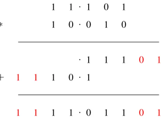
2.1 Hardware and semantics preliminaries 7 1 1 . 1 0 1 1 0 . 0 1 0 ∗ . 1 1 1 0 1 1 1 1 0 . 1 + 1 1 1 1 . 0 1 1 0 1
Figure 2.1: A multiplication in fixed-point representation, as taught in school.
The fixed-point arithmetic The main advantage of fixed-point representation is that addition and subtraction are done without any error. The only case in which an error can happen is when the sum of two numbers exceeds the maximal capacity. Technically this is not a rounding error but rather an overflow error.
The multiplication of two fixed-point numbers generates both rounding and overflow error as illustrated in figure 2.1. The rounding is an inherent problem of finite precision representation. But, here it can easily lead to an underflow exception: the result is rounded to 0. Rounding to 0 a non zero number is problematic since it cannot be used to divide a number while it is possible with the exact number. On the other hand, the overflow (i.e. the loss of the most significant bits) is the most serious problem of this representation. Indeed, the returned number is not related anymore to the exact number, so that most of the time it leads to a fatal error. These two problems, underflow and overflow, are permanent problems to the developer since the amplitude of representable numbers is just 2nwhich is very limiting.
2.1.2 The floating-point representation
Representation of reals in an efficient way is a central problem in computer science. Reals are manipulated so often that the processor contains a part dedicated to manipulate them. This part is called the floating point unit (FPU). Since errors on representation of reals are a big issue, this unit has been fully optimized and therefore it is more complex to explain than fixed point representation.
As we explained, there are two main problems with fixed-point representation. On one hand, to define their type, we need an additional parameter: the number of digits that stands for the fractional part. On the other hand, avoiding overflow and underflow errors requires a special attention. To avoid these two issues, the floating-point representation allocates some bits to
8 Robustness 2.1
define the exponent.
There are several kinds of floating-point representations that are used depending on their size. Here, we detail only the most used one called “doubles” which stands for double precision floating-point number.
Doubles use 64 bits: one bit s for the sign, another one e0for the sign of the exponent, 10
bits e1, . . . , e11 for the absolute value of the exponent and 52 bits m1, . . . , m52for the mantissa.
The number d represented in this way is: d= (−1)s 1 + 52
∑
i=1 mi2−i ! e(−1)e0∑10j=1ej2jIn addition, there are some additional combinations of bits that represent errors like “infinite result” when a division by zero occurs.
Full precision for atomic operators in floating-point representation There are two kinds of rounding errors. The first ones is intrinsic to the finite precision representation, i.e., any time the result of a computation would be a non representable number then it has to be rounded to a representable number. For instance,√2 cannot be represented by a finite number. The other kind of error is due to a wrong result for the computation, i.e., the returned result is not the closest representable number of the mathematical result.
Definition 2.1.1 (full precision). An implementation of a function is “full precision” if there is no representable number in between the provided result and the exact one.
The main goal that motivated the creation of floating-point numbers was to provide full precision for all mathematical operators. Another objective was to be able to specify which one of the two admissible results (the greater or the lower one) has to be returned such that the programmer can fully determine which result will be returned. These two goals have been achieved years ago: the IEEE standard 754 [IEE08] for floating-point arithmetic certifies that the returned result for any one step operation is one of the closest numbers that the floating point can represent. This standard also proposes several policies for rounding: to return the greater or the lower number, to return the closest to zero number or to return the number closest to the true result.
Addition and subtraction While fixed point representation adds no rounding error for addi-tion, floating point numbers rounds result each time the ratioa/bis outside of [−0.5,−2]. Indeed,
2.1 Hardware and semantics preliminaries 9
sign) then the final exponent will be ea+ 1, so the last bit is lost. If ea> ebthen either ea+b= ea
or ea+b= ea+ 1. In that case, the last ea− ebbits of b are not used to compute a + b.
Multiplication and division Multiplicative operators have a much better implementation with floating-point than with fixed-point representations since the exponent will change in order to always keep the most significant bits. So, in this representation, there is no useless zeros or strong bit truncation. The result is not always the exact one however. A rounding happens at least each time we divide by a number such that the rational result has a quotient which is not a power of two. In addition, the multiplication of the two mantissas is a multiplication of two integers: the returned result is twice as long as the initial numbers. So, since the size of the mantissa is also 53, half of the least significant bits are rounded.
Exponentiation Exponentiation is also considered as a primitive by the IEEE standard. How-ever, the actual computation is done through three steps according to the following formula:
xy= 2log2(x)y
To be able to provide full precision for this composed operations, processors use a larger internal floating-point representation with 80 bits such that rounding errors remain small and do not affect the final result.
2.1.3 Semantics of programs. Definitions and notations
As we have seen, the actual problem of rounding numbers does not occur when there is just one operation that is performed: the floating-point semantics grants that the error is negligible proportionally to the value. As we will see, the situation is different for a whole program. But in order to speak about programs we need to introduce first some definitions and notations. Programming language Programming languages allow programmers to produce machine code without worrying about the actual machine instructions of a specific processor. The more elaborate is the language, the more high-level is the code written by the programmer. In our study, we choose to describe programs through a pseudo language, so that we can highlight the arithmetic operations.
We represent functions with the following syntax: f (x , y ){
...
10 Robustness 2.1
}
Here f is he name of the function and x,y are the parameter of the function. The instruction return z; indicates that the function returns z (which has to be defined in the body of the program).
For instance, the following code is an implementation of the square function. square ( x ){
return x * x ; }
The following code, is also an implementation of the square function. square ( x ){
y =( x +1);
return x * y - x ; }
In general, given a mathematical function, there is not a unique implementation of it. While two implementations are equivalent in theory, their rounding errors have no reason to be the same.
To make the link between a program code and a mathematical function, we use an inductive definition called denotational semantics. We use the notation [[instructions;]] to represent the semantics of the code instruction. The base case are the variables and the constants. The semantics of a variable x is its value (we will describe later which one). The semantics of a composite expression, like x + y, is obtained from the semantics of the components. For instance, [[x + y]] = [[x]] + [[y]].
This definition is non ambiguous, while we consider there is no rounding. But, for our purpose we need to differentiate between the intended computation i.e. where operations are made on reals and the actual computation where operations are the ones described by the finite-precision arithmetic. To distinguish between them, we note [[x + y]]′the result of the
computa-tion in the finite precision system.
When we have already set that [[instructions;]] = f where f is a function, we will use the more readable notation f′instead of [[instructions;]]′such that [[instructions;]]′= f′.
2.1.4 Problems induced by the rounding error
We have briefly presented finite-precision implementations and the semantics of programs. Now, we present some of the challenges raised by floating-point representation. Indeed, while a single
2.1 Hardware and semantics preliminaries 11
operation grants the most accurate result, a succession of several operations may lead to critical deviations.
Difficulty to compute the exact error Finite representations do not enjoy traditional proper-ties [Gol91]. In particular, the associativity of the addition is broken in floating-point represen-tation. Indeed, when computing (a + b) + c, first a + b is rounded then c is added, while for computing a + (b + c), (b + c) is rounded first. So, if b = −c and a ≪ b, a + b is rounded to b such that the final result is 0 , while b + c = 0 so the result of a+(b+c) is a.
This kind of errors is unpredictable for the developer since compiler optimizations may change the order the operations are executed. Thus, if the programmer writes in a high-level programing language, it might be impossible to predict the errors that the compiled code will make. That is one of the reasons why we do not try to compute the error but just to compute a bound on it.
Absolute or relative error? When dealing with rounding errors, we would like to ensure a property like “the error never exceeds p percents of the exact number”. Such a property, however, is not compositional. Indeed, as we have seen in the previous example, if an addition is made between two numbers a and b such that the ratiob/ais big, then adding −b increases the
relative error significantly. Since such a phenomenon is not easily traceable (except in case of a simple addition of positive numbers), we prefer in our study to concentrate on absolute errors (i.e. we do not provide a percentage but the deviation itself).
Absolute errors are harder to compute when an algorithm is mostly based on multiplications. Indeed, if we know some bounds ε on the absolute error on a and b then the error after the multiplication is aε+bε+ε2, which is not bounded as long as a and b are not bounded. However,
in the algorithms we study this is not problematic because we never do iterative multiplications and because there always exists a maximal bound on all inputs values. In addition, we present an example to show that in some cases relative errors are also hard to compute and can lead to weaker results than absolute errors.
Example 2.1.1 (Robustness breaks with a simple iterative loop). In this example, we stress that non robust behaviors (i.e., behaviors vulnerable to rounding errors) can emerge even from simple and regular programs. Consider the following code.
geo(x0,x1,n){ u=x0;
v=x1; w=0;
12 Robustness 2.2 for(i=0 to n){ w= a*v + b*u; u= v; v= w; } return w; }
This code, in the exact semantics, computes the value un+1of the sequence defined by: u0= x0,
u1= x1 and
un+1= aun+ bun−1
A mathematical theorem states that
un= Arn1+ Brn2
where r1and r2are the distinct roots of the quadratic
X2− aX − b
and A and B are fixed by the initial condition.
Now, assume that a and b are representable numbers such that r1< 1 and r2 > 1. Then,
assume we run this program with parameter x0 = 1 and x1 = r1. In that case, we have A= 1
and B= 0. So, in the exact semantics, a big value of n provide a result close to 0. In the finite precision semantics however, if r1 is not representable then the input will be an approximation
r′1. Since the initial conditions are changed the B value is not zero anymore butε. If n is big, the term in Arn1tend to zero while the term inεrn
2due to errors tend to infinity.
Finally, it is not possible to efficiently bound the relative error of this program due to just one critical case, while the absolute error is pretty regular for all values.
2.2
Quantitative analysis
A quantitative analysis means that we measure the error made by the finite representations. There are several choices to do this measure. Before presenting our definitions, we explain the reason of our choice.
Our goal in chapter 3 is to provide a method to compute the probabilistic information leakage of a program once a quantitative analysis of the error has already been performed. In chapter 4, we provide a method such that once some parts of the code have been analyzed then it is
2.2 Quantitative analysis 13
possible to analyze the whole program from the point of view of its robustness to errors. We are interested in some formulation of robustness which can be performed by traditional tools and which can be easily manipulated from a mathematical point of view.
2.2.1 Static analysis
The term “static” means that the analysis is done without executing the program but just by processing the code of the program. Static analysis provides over approximations of the studied property. In our case, this means that a bound on the error is not necessary the optimal one. A static analysis is better than a battery of test cases since it provides a result valid for the whole domain while dynamic testing may fail to test some cases.
There are two main methods to do a static analysis of a program, whatever the analysis is about. We briefly present them.
Logic based proof This technique has been introduce by Hoare [Hoa69] and has now several variants. The principle of this analysis consists on considering any instruction as a transforma-tion between preconditransforma-tions and post conditransforma-tions. The main feature of Hoare logic are the Hoare triple that describe the execution of one instruction. A Hoare triple is written as:
{P}I{Q}
where P is a formula that is the precondition, I is the instruction and Q is the post condition. From these triples it is possible to derive other triples with inference rules. For instance, the following rule allows to derive a triple for a sequence of instructions.
{P}I1{Q} {Q}I2{R}
{P}I1; I2{R}
Abstract interpretation Abstract interpretation [CC77] aims at providing over approxima-tions of all possible behaviors of a program. In abstract interpretation, the semantics of a pro-gram, i.e., [[.]]′, is called the concrete semantics. The domain whose elements constitute the over
representations of values and states of programs is called “abstract domain”. For instance, an ab-straction of the exact value of a variable can be an interval in which this variable belongs. Once an abstract domain is defined, the abstract interpretation computes the abstraction that results from the previous abstraction by applying the instruction. For instance, if our abstract domain consists of intervals, from an interval [a,b] the instruction x=2*x; leads to the interval [2a,2b].
14 Robustness 2.2
2.2.2 Input-output relation
There are several kinds of properties that may be interesting for studying the errors due to fi-nite precision. The first question when we study error is the sensitivity of the output for small variations of the input. Indeed, even if a program computes the result in full precision, the input value, in general, comes from either a physical value or another computation and is not the exact value. If the program has an erratic behavior then even a small error on the input leads to a big error to the output.
A weak property that can be defined about the relation between input and output is continu-ity:
Definition 2.2.1 (continuity). A function f : R→ R is continuous, if ∀ε > 0 ∀x,x′∈ R ∃δ |x − x′| ≤ δ =⇒ | f (x) − f (x′)| ≤ ε
The continuity property ensures that the correct output can be approximated when we can approximate the input closely enough. This notion of robustness, however, is too weak in many settings, because a small variation in the input can cause an unbounded change in the output.
On the other hand, a function which is not continuous has little chance to be robust. Since various regularity properties imply continuity, it is sometime useful to prove a function is not continuous in order to avoid to waist time trying to prove these properties.
A stronger property is the k-Lipschitz property.
Definition 2.2.2 (k-Lipschitz). A function f : Rm→ Rnis k-Lipschitz, according to the distances
dmand dn, respectively, if
∀x,x′∈ Rm dn( f (x), f (x′)) ≤ k · dm(x, x′)
The k-Lipschitz property amends this problem because it fixes a bound on the variation of the output linearly to the variation of the input.
The k-Lipschitz property has been used by Chaudhuri et al [CGL10, CGLN11] to define robustness. To prove a program to be k-Lipschitz, they first prove the function is continuous then they prove the function is piecewise k-Lipschitz while they compute k .
However, the k-Lipschitz property does not deal with algorithms that have a desired precision e as a parameter and are considered correct as long as the result differs by at most e from the results of the mathematical function they are meant to implement. A program of this kind may be discontinuous (and therefore not k-Lipschitz) even if it is considered to be a correct implementation of a k-Lipschitz function.
2.2 Quantitative analysis 15
1 2 3 4
1 2
0
Figure 2.2: The function g−1and its approximation
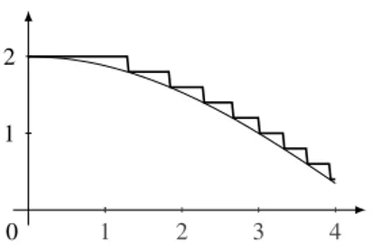
Example 2.2.1. The phenomenon is illustrated by the following program f which is meant to compute the inverse of a strictly increasing function g: R+→ R+ whose inverse is k-Lipschitz for some k.
f(i){ y=0;
while(g(y) < i){ y = y+e; } return y; }
The program f approximates g−1with precision e in the sense that
∀x ∈ R+ f(x) − e ≤ g−1(x) ≤ f (x)
Given the above inequality, we would like to consider the program f as robust, even though the function it computes is discontinuous (and hence not k-Lipschitz, for any k). We illustrate in figure 2.2 how the functioncos is approximated by such an algorithm.
This example motivates our definition of input output relation that we will define later.
2.2.3 Dealing with several variables
The previous definitions are valid only for functions with one argument and one output. How-ever, to be general, we should give definitions that are applicable to programs with several argu-ments.
In general, a program may have an arbitrary number of arguments. For instance, a program sorting a list deals with all the numbers the list contains. Another example is a program receiving a stream of physical data every second. These two examples are not analyzed in the same way however. Indeed, a program that receives a stream and agglomerates the results (like a program that sums all entries) has a fixed memory size. In that case, we can consider that the program has only one variable that receives all the values, as illustrated by the following code.
16 Robustness 2.2
sum (){ y = 0 ;
while( input not empty ) y = y + new_input (); return y ;
In that case, we can consider the program only has one internal variable y while the input vari-ables are the outputs of the new_input() instruction. With this interpretation, inputs errors are seen as internal errors of the instruction new_input() instead of input errors of the program.
The case where the program can use an arbitrary large memory is more difficult. However, the memory capacity of any device is limited and allocation of too much memory can crash the program. So, to prove the robustness of the program, it is necessary to prove that this allocation will be bounded, and therefore we can only consider the cases up to the maximal size. On the other hand, dynamic allocation slows down the execution of the program. Since robustness analysis is mostly made for critical system like embedded system that have to be fast and simple, these kind of programs with dynamic allocation are not really studied and we do not study them either.
Therefore, we restrict our study to programs that deal with a fixed number of variables. To be able to do an accurate analysis of the propagation of error, it is interesting to track each variable individually.
For instance, an approach used by Majumdar et al in [MS09, MSW10] consists on formulat-ing robustness with the followformulat-ing definition. A function f is (δ,ε)-robust on the i-th input, if a variation of at most δ on the i-th variable while all other are identical, makes a shift of at most ε. Another approach has been considered to deal with error annihilation when computations add then remove the same quantity. For instance, the expression 3y − y can only double the initial error from y, while 3y − x can have an error which is the sum of the deviations of 3y and x.
Studying how robustness depends on each variable is very useful to get better approxima-tions of the error. However in our case, we use results coming from automated analysis to obtain either a more complex property than just error deviation (the differential privacy in chapter 3) or a property about a more complex program (in chapter 4). To be able to use any kind of former analysis which can be more or less precise and to provide general results, we need a general enough definition. That is why we prefer to use the notion of distance that aggregates errors from several variable into one quantity. Formally, a distance is defined as follows:
Definition 2.2.3 (Metric space). A metric space is an ordered pair(M, d) where M is a set and d is a distance on M, i.e., a function
2.2 Quantitative analysis 17
d: M × M → R such that for any x, y, z ∈ M, the following holds: 1. d(x, y) ≥ 0 (non-negative),
2. d(x, y) = 0 ⇐⇒ x = y (identity of indiscernibles), 3. d(x, y) = d(y, x) (symmetry) and
4. d(x, z) ≤ d(x,y) + d(y,z) (triangle inequality) .
Since we are interested in programs computing with real valued inputs and outputs, we mostly use metric spaces based on Rm, the cross product of R m times where m ∈ N.
The set Rmis a normed vectorial space [Rud86]. This means we can add two vectors, we
can multiply any vector a vector by a scalar (an element of R) and there is a norm on it. In the case of Rm, if x = (x
1, . . . , xm) and y = (y1, . . . , ym) are in Rm, then x + y is defined components
by components :x + y = (x1+ y1, . . . , xm+ ym). The scalar multiplication is done the same way:
λx = (λx1, . . . , λxm). We also use the notation x − y that stands for x + (−1) · y.
Finally, norms are defined as follows.
Definition 2.2.4 (Lp norm). For n ∈ N and x = (x1, . . . , xn) ∈ Rm, the Lpnorm of x, which we
will denote bykxkp, is defined as
kxkp= p s n
∑
i=1 |xi|pFrom these norms, it is possible to define all natural distances (the one that only rely on the normed vectorial space structure).
Definition 2.2.5 (distance). The distance function corresponding to the Lpnorm is
dp(x, y) = kx − ykp.
We extend this norm and distance to p = ∞ in the usual way: kxk∞= max
i∈{1,...,n}|xi|
and
d∞(x, y) = kx − yk∞.
When clear from the context, we will omit the parameter p and write simply kxk and d(x,y) for kxkpand dp(x, y), respectively.
18 Robustness 2.2
2.2.4 Internal rounding error
The relationship between inputs and outputs does not give any information on how big the com-putational error can be inside the program itself. If we prove that the exact semantics of a program is k-Lipschitz, it means that if the input contains an error e then the result amplifies this error by at most k. However, an arbitrary large error (i.e., not function of e) can still appear as a consequence of rounding errors associated to the computation.
On the other hand, even if we prove that the finite-precision semantics of the program is k-Lipschitz, this does not mean that the computation is close to the exact function. We can imagine for instance a program that, due to errors, returns always 0 while the function is supposed to return a less trivial result.Such a program is 0-Lipschitz but is not robust.
In general, to know a robustness condition between inputs and outputs is necessary to have a robust program, but it is not sufficient. So, to analyze internal errors, we need to develop other specifications than just a property about the function. Mainly, we need to consider a relation between both the exact semantics and the finite precision semantics of the program. Both abstract interpretation [GP11] and Hoare based logic [BF07] study internal errors through pairs consisting of the value in the exact semantics and the finite precision semantics.
In abstract interpretation, the concrete semantics is a triple (r, f ,e) where r is the real value (in the exact semantics), f the actual floating point value and e is the error (e = f − r). The abstract domain consists of the values of the following form:
f = r +
∑
i
aiεi
where the εirepresent any value in the interval [−1,1] and the aiare real-valued scale factors.
In the Hoare logic, the preconditions and the post conditions are properties that state the maximal distance between the two semantics.
Since the former approach also implies a maximal distance (the sum of the ai) and that
distances are nice to be manipulated mathematically, we will consider the following definition. Definition 2.2.6 (L∞norm (on functions)). The L∞norm of a function f : Rm→ Rn, according
to a given norm Lpon Rn, is defined as:
k f k∞= sup
x∈Rmk f (x)kp
.
This definition makes an implicit reference on the norm k · kpused to measure single vector.
In our study, we will mostly use the k · k1norm. From the last definition, we can also define the
2.3 Our approach to robustness 19
Definition 2.2.7. Let f and f′two functions Rm→ Rn,
d∞( f , f′) = sup
x∈Rmk f (x) − f (x)kp
.
2.3
Our approach to robustness
In this section, we provide the definitions we will use in the next chapters as well as the properties that these definitions enjoy.
2.3.1 Input-output relation
First, we consider only the relationship between inputs and outputs of the function. As we have explained in section 2.2.2, some work in the literature consider the k-Lipschitz property. How-ever, example 2.2.1 illustrates an example where a function which is not k-Lipschitz has to be considered robust because the discontinuity are less than some small value. In [BF07], they amend this problem by considering a third semantics in addition to the exact and the finite pre-cision one: the so-called intended semantics. Here, we prefer not to introduce another semantics but to consider that the implemented function is close up to ε to a regular function.
Definitions
The definition we propose is the following.
Definition 2.3.1 (The P(k, ε) property). Let (Rm, d
m) and (Rn, dn) two metric spaces. Let f :
Rm→ Rn, k, ε ∈ R+∪ {0} , we say that f is P(k,ε) if
∀x,x′∈ Rm, dn( f (x), f (x′)) ≤ k · dm(x, x′) + ε
This property is a generalization of the k-Lipschitz property, which can be expressed as Pk,0.
In general, for ε > 0, P(k,ε) is less strict than k-Lipschitz and avoids the problem illustrated in example 2.2.1. The function in that example,in fact, is Pk,e.
In some cases, a large deviation on the input may cause the deviation on the output to go out of control, independently from “how well” the program behaves on small deviations. In general, we hope to maintain the deviation small, hence it is useful to relax the P(k,ε) definition to consider only inputs that are quite close (up to some δ). So we provide the following P(k,ε,δ) definition:
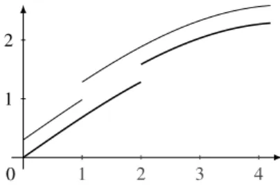
20 Robustness 2.3 1 2 3 4 1 2 0 Figure 2.3: A P(k,ε) function Definition 2.3.2 (The property P(k, ε, δ)). Let (Rm, d
m) and (Rn, dn) be metric spaces , f : Rm→
Rnbe a function, k, ε ∈ R+, and letδ ∈ R+∪ {+∞}. We say that f is P(k,ε) if:
∀x,x′∈ Rm, dm(x, x′) ≤ δ =⇒ dn( f (x), f (x′)) ≤ kdm(x, x′) + ε
This new definition is an extension of the former one since P(k,ε) = P(k,ε,∞). Properties of our notions of robustness
We, now, provide some useful properties about the above definitions. First, we relate the P(k,ε) property to the k-Lipschitz property.
Proposition 2.3.1. If f is k-Lipschitz andk f′− f k∞≤ ε, then f′is P(k, 2ε).
Proof. Consider the triangular inequality
dn( f′(x), f′(y)) ≤ dn( f′(x), f (x)) + dn( f (x), f (y)) + dn( f (y), f′(y))
Then since f is k-Lipschitz:
dn( f′(x), f′(y)) ≤ dn( f′(x), f (x)) + kdm(x, y) + dn( f (y), f′(y))
Finally, since k f′− f k∞≤ ε:
dn( f′(x), f′(y)) ≤ ε + kdm(x, y) + ε
which is the definition of P(k,2ε).
Regular functions in the intended semantics are k-Lipschitz, we introduced the P(k,ε) prop-erty to weaken the k-Lipschitz propprop-erty in order to also accept functions that are close to their intended semantics. This property states that functions close up to ε to a k-Lipschitz intended function are actually P(k,2ε).