Advanced demand response solutions based on fine-grained load control

HAL Id: hal-01092441

https://hal.archives-ouvertes.fr/hal-01092441

Submitted on 8 Dec 2014

HAL is a multi-disciplinary open access

archive for the deposit and dissemination of

sci-entific research documents, whether they are

pub-lished or not. The documents may come from

teaching and research institutions in France or

abroad, or from public or private research centers.

L’archive ouverte pluridisciplinaire HAL, est

destinée au dépôt et à la diffusion de documents

scientifiques de niveau recherche, publiés ou non,

émanant des établissements d’enseignement et de

recherche français ou étrangers, des laboratoires

publics ou privés.

Advanced demand response solutions based on

fine-grained load control

Rim Kaddah, Daniel Kofman, Michal Pioro

To cite this version:

Rim Kaddah, Daniel Kofman, Michal Pioro. Advanced demand response solutions based on

fine-grained load control. IEEE IWIES 2014, 2014, pp.38 - 45. �10.1109/IWIES.2014.6957044�.

�hal-01092441�

Advanced demand response solutions based on

fine-grained load control

Rim Kaddah

,Daniel Kofman

and Michal Pioro

Emails:{rim.kaddah,daniel.kofman}@telecom-paristech.fr

†_{Institute of Telecommunications, Warsaw University of Technology, Poland} ‡ _{Department of Electrical and Information Technology, Lund University, Sweden}

Email: michal.pioro@eit.lth.se

Abstract—We consider demand response solutions having the

capability to monitor different variables at users’ premises, like presence and temperature, and to control individual appliances. We focus on the optimal control of the appliances during time periods where the available capacity is not enough to satisfy the demand generated by houses operating freely. We propose an approach to define the utility of appliances as a function of monitored variables, as well as control schemes to optimize this utility. Global optimums can be reached when a centralized entity (i.e., an aggregator) can gather information from each user and control each individual appliance. This may not be always possible, for example for privacy and/or scalability reasons. We therefore consider, in addition, a system where decisions are taken partially at a centralized site (global power allocation per home) and partially at customer premises (sharing of the allocated power among local appliances). Performances of proposed control mech-anisms are evaluated and compared. We show the potential value of introducing demand response mechanisms at fine granularity.

I. INTRODUCTION

Present trends in the eco-system of electricity operators, like the growing penetration of renewable intermittent energy sources and the increasing number of end-users playing active roles, have increased the requirement for advanced demand response solutions.

The Internet of Things paradigm and its specific imple-mentations - for example in smart houses and smart buildings - enable new service models for electricity operators as well as innovative demand response approaches. This general idea is gaining momentum, as it is attested by the recent acquisition of Nest by Google (and by the related business models established with electricity operators).

In the present paper we introduce an approach for imple-menting advanced demand response solutions at a potentially broad geographical scope that: i) can work at the level of users’ appliances, ii) can take into consideration data monitored at user premises, like presence and temperature and iii) based on this information, optimizes the total provided utility (e.g. at a neighborhood scale) under fairness constraints. Definitions of ”utility” and ”fairness” for this specific context are provided in the paper, as well as the way to model them.

In [6] the authors have introduced a family of new service models for the provision of electricity, in particular to face

*This author has carried out the work presented in this paper at LINCS (www.lincs.fr)

periods of time during which it is not possible to cope with all the demand, either because of technical or economic reasons. The proposed service models allow significantly limiting the impact on quality of experience during such time periods by avoiding coarse-grained control mechanisms (like rolling blackouts) or high costs. Based on the general architecture proposed in the document, available power can be distributed in a smarter way, at a fine granularity, taking into consideration the relevance of each appliance for the end-users. In particular, the proposed architecture leverages the capabilities of the Internet of Things paradigm. The mechanisms we propose in the present paper can be embedded on this general framework as an implementation of one of its key building blocks, but their scope of application is much broader.

The methodology proposed in this paper is motivated as follows. In case of scarcity of resources, the general target is to minimize the impact on quality of experience. In order to trans-late this general statement into autonomous taken decisions leading to optimal power allocation and appliances control, we need first to model the utility, from the end user point of view, of receiving a certain amount of power. Therefore, in this paper we first provide a typology of appliances and define their utility as a function of different relevant variables (like ambient temperature for the control of a heating system). We also model the evolution of these variables as a function of the provided power in order to be able to represent how the decisions taken at a given time will impact the user perceived utility in the future.

Based on the proposed model of utility and on the dynamics of the system variables (e.g. evolution of temperature as a function of the power provided to the heating system), we propose different approaches for allocating power to the vari-ous appliances of the different clients of a given geographical zone characterized by the electric network infrastructure. We consider control systems that work at different granularities, ranging from power allocation to individual appliances to total power allocation to end-users. We also consider ahead of time and real-time approaches. Supposing time is slotted, we call ahead of time those approaches where the decisions are taken at the beginning of a time period for its whole duration. We call real time approaches those where for a given time period, control decisions are taken at each time slot without knowledge of how exogenous variables (like total available capacity) will

evolve in future time slots.

For specific use cases, we optimize the control system for the various proposed control approaches and compare the results. We show the potential high impact of the presented solution.

The paper is organized as follows: Section II presents related work. Section III introduces the problem and presents the general framework as well as the taxonomy of appliances, utility definitions and control schemes we propose. In Section IV, we instantiate a specific system and propose a model that allow us, for this specific system, to evaluate and compare the performances of the various control schemes we propose. In Section V, we present a numerical analysis of the model which outcomes provide insight on the behavior of the proposed control schemes. Conclusions and future work are presented in Section VI.

II. RELATED WORK

The topic of Demand Response has motivated a large set of contributions during the last years. Demand Response approaches can be grouped in two categories: pricing based and direct load control. The approaches in the first category try to induce the expected users’ behavior through dynamic pricing incentives and provide no strict guaranties on the outcome. On this group we can cite [7], [3], [4], [9]). In [7], the authors propose a taxonomy of appliances and a pricing scheme that takes into account utility functions of the appliances being served. In the present paper we propose a different taxonomy of services that we consider better adapted for the definition of utility functions, as explained in Section III-D. In particular, it enables taking into account in a simple way the criticality of a given appliance as seen by a given user. We also propose a related general approach for defining utility functions.

The approaches in the second category, in which we are interested, enables Distribution System Operator (DSO) or aggregators to directly control the load. Load can be con-trolled at different granularities, e.g. per user or per appliance. Previous works on direct per appliance load control focus on specific types of appliances. For instance, the authors in [2] consider the control of shiftable loads. In [15], [14], the authors show the high value of exploiting the capability to reduce power allocated to elastic appliances. This last paper focuses on peaks reductions whereas we focus on complying with the available total capacity. A wide range of work focused on Thermostatically Controlled Loads (TLCs) ([10], [8], [11], [13], [5]). The approach presented in this paper is generic, and applies to any control granularity and any type of appliances. To our knowledge, no generic framework was proposed that allows joint control of different types of appliances in case of direct load control involving an aggregation of homes. In this work, we choose to use utility functions to model the flexibility (e.g., shifting capabilities, payback effect) and relevance for the users of all types of controlled appliances. Utility functions were previously used in the literature to measure social welfare when designing pricing schemes and are generally considered as (convex) functions of power (e.g., [12]). Our approach is similar to [7] but more general: utility is represented as a func-tion of several relevant variables (endogenous and exogenous to clients’ environment), which in particular enable evaluating

the impact on quality of experience of the allocated power, and we differentiate appliance usage from its operation constraints. In [1] the authors focus on how aggregators can leverage in the energy market the flexibility that can be provided by clusters of users. For this and other contributions that have been published on the topic, our proposals enable increasing the available aggregated flexibility.

III. PROBLEM STATEMENT AND PROPOSED SOLUTIONS

A. Problem statement

Power grids are evolving fast but are still lacking mecha-nisms for fine-grained control of power allocation. In this paper we consider advanced frameworks, like the one presented in [6], which enable controlling the demand at different granu-larities, including at a per appliance level, during periods of generation shortage.

We consider two functional groups in charge of demand control, one located at a Distribution System Operator (DSO) or aggregator site and the other one at user premises. The design of the demand-response mechanisms implemented through these two functional groups targets energy efficiency as well as satisfying users’ expectations. Complexity arises because, on the one side, those two global objectives could be contradictory and, on the other hand, theoretic optimal solutions may not be feasible (e.g. for scalability reasons) and several non-technical factors have to be considered (e.g. privacy issues may constrain the data that can be made available to the DSO or aggregator).

We can summarize our problem statement as follows: Under the hypotheses that an advanced architecture enabling demand control at fine granularity is deployed and that a set of variables are monitored at user premises, we search demand control mechanisms for energy efficiency and users’ satisfaction under different constraints of scalability and of the users’ data dissemination scope.

B. Solutions framework

We focus on time periods where the global demand exceeds the available capacity. We call DEa andDEu the functional

groups at the DSO/aggregator side and at the user side, respec-tively.DEu is aware of the state of the variables monitored at

user premises and receives control decisions fromDEa. When

relevant to a specific control case,DEucan transmit all or part

of the data he gathered to DEa.

We consider different demand control approaches. They can be classified in two families. In the first family, DEa decisions

are taken at the granularity of users, without any knowledge on individual appliances nor on the state of monitored variables. At each decision time, it allocates to each user a maximum power (which could be different for different users) for a certain time period. Based on this limit, DEu controls the

demand of each appliance. In the second family,DEa has full

information and directly controls the appliances.

In order to quantify energy efficiency and users satisfaction, we define for each appliance a utility function. The utility may depend on the monitored variables (like presence or tempera-ture) and on exogenous variables (like outside temperatempera-ture).

The models we introduce in the following section target maximizing the total utility under different types of system constraints and taking into account fairness considerations. We do not directly focus on the revenues of the players. Nevertheless, one can expect that if well performing pricing models are defined, reaching maximum users’ utility leads to maximum gains.

C. Proposed control schemes

In the following, we propose different control schemes and we compare their performances. The choice of a scheme will depend as well on the different service models and corresponding tariff schemes that can be associated to them.

1) Global Maximum Utility: The Maximum Utility scheme supposes DEa has full information and decides how much

power to allocate to each appliance in order to maximize the total utility, means the sum of the utilities of each appliance of each user. We call this schemeM U

2) Global Maximum Utility under fairness constraints:

This scheme, that we name F M U , also supposes that DEa

has full information. It maximizes the total utility in a restricted domain where the minimum of the utilities of all users is max-imized (see Section IV-B for a formal definition). We consider this scheme in order to introduce fairness. In fact we assume here a specific fairness definition1, which seems in particular appropriate for the case of homogeneous users (homes with similar characteristics). For the case of heterogeneous users, depending on different considerations that we will not treat here, it can be argued that a scheme where max-min is applied to the utility divided by the number of inhabitants (or square meters) would be fairer.

3) Local maximum utility under homogeneous capacity constraints: In this scheme, users are grouped into classes. Each class receives a certain amount of power based on a parameter that is associated to the class at the configuration time of the system (for example, the allocation may be a function of the maximum power authorized for the users of the class in nominal conditions). At each decision time, DEa allocates to each user the power allocated its class

divided by the number of users in the class and transmits the corresponding information to each DEu that, based on this

limi, takes control decisions in order to maximize local utility.

We name this scheme LM H.

4) Rolling Black-Outs: In this scheme, the power allocated to each user byDEa is either the maximum subscribed power

or zero. We analyze a simple approach to introduce fairness in power allocation, which will be explained in the section devoted to presenting the optimization models. As in the previous schemes, each DEu controls the appliances in order

to maximize local utility and to respect the allocated power. We call this scheme RB.

1_{Notice that this is not max-min fairness; nevertheless, the minimum utility} provided to a given user will be the same as in max-min fairness. We do not introduce max-min fairness because max-min fair solutions of the problem we define may not exist, as can be understood from the formal problem stated in Section IV-B

5) Decisions time: The DSO or aggregator may be able to forecast the starting time and duration of a starvation time period (e.g. predicted extreme weather conditions). In this case, the power allocation may be done at the beginning of the time period for its whole duration. In other cases, starvation periods are not known a priori. Moreover, optimizing the system for the whole period under the studied constraints that take into account the dynamics of different variables (like the temperature in the house) may not be scalable in certain contexts.

Therefore, we analyze and compare the 2 first above-presented schemes both in the cases of ahead of time and real-time optimization.

D. Appliances’ Taxonomy and Utility Functions

In this section, we first present a taxonomy of appliances from which one can derive the type of control that can be applied to each given appliance (its flexibility). The taxonomy also provides the rationale for the utility functions we propose afterward.

1) Taxonomy : We consider that, for the purpose of modeling demand control mechanisms and users satisfaction, appliances should be classified based on the 3 following criteria.

a) Criterion 1 - Usage: We propose grouping appli-ances based on 3 general types of usage:

• Interactive demands

Interactive demands are those that are directly trig-gered by end users and, when possible, should be served immediatly. Obviously, the utility of those appliances depends directly on the presence of in-habitants. Lighting and TV are typical examples of interactive loads.

• Background loads

Background loads are those in charge of controlling the value of variables like the temperature in a room, in the water-heater or inside the fridge. They are usually shiftable, which means that shifting (up to a certain limit) the time at which the expected energy is provided do not significantly affect the quality of experience. They may depend on presence but also on exogeneous variables (e.g. related with the weather). The value of feeding such loads depends on the distance between the targeted and present values of the variables being controlled and also on the dynamics of the variable (how the variables evolve in time as a function of the power provided to the appliance). Subclasses can be defined depending on the level of inertia of the controlled variables. For example, a heating system has more inertia than an air-conditioning cooling system.

• Program based loads

Program based loadsare those that have well defined operation cycles that can be programmed. The value of feeding these appliances is related with the capacity of completing a program. They are usually shiftable, but in most cases they are not elastic. They can be classified on those than can be stopped before of

the end of the cycle and those for witch such an event may generate some damage. Typical examples of this category are washing machines and charging systems for electric vehicles. The quality of experience depends, in particular, in the distance between the expected and actual start time and termination time of an operation cycle, as well as on the level of respect of the constraints on acceptable interruptions and on the total provided service (e.g. charging) during the cycle.

b) Criterion 2 - Criticality and preferences: Appli-ances can be differentiated by their criticality. We can de-fine three levels of criticality namely, ”Critical”, ”Basic” and ”Others”. The first category comprises demands that have to be accommodated under any circumstances (e.g., home medical equipment that have to operate when needed). Basic demands are generated to accommodate important needs that will significantly affect users’ well-being. (e.g., a certain level of lighting, space heating during especially cold weather). Demands that fall into the ”Others” category are those that can be abandoned without significantly affecting home residents’ well being (e.g. entertainment). Moreover, users may provide a priority ordering of loads depending on their own perception of the importance of the appliances.

c) Criterion 3 - Electrical characteristics and power flexibility: This category describes electrical characteristics of loads (e.g., resistive, inductive, storage) that may impose operation constraints. For resistive loads, reducing power will affect the quality of experience but not avoid functioning. In many cases resistive loads are elastic and therefore reducing allocated power will just delay the provision of the service (for example, a water-heater will take longer time to reach the desired water temperature). Inductive loads are usually less flexible.

2) Utility Functions : As mentioned, the general approach we propose relies on the definition of utility functions. Based on the presented taxonomy, we propose a 3 steps methodology to derive utility functions and adequate control decisions for any type of appliances.

1) Define normalized utility functions for the different types of usages (Criterion 1). The following are just examples of functions that could be used. Since for interactive loads utility depends directly on power allocated and the presence of inhabitants, it can be defined as an increasing in power and piecewise linear function with slopes that decrease since the marginal utility decreases after having satisfied a group of houses needs. For background loads, utility is de-pendent on the value of some controlled variables; it can therefore be defined as a monotone piece-wise linear function in these variables with different slopes between minimum, preferred and maximum tolerable thresholds of the controlled variables. Since for Program based loads, utility is related with the completion of a program, it can be expressed as a function of total required energy to complete a program and of the distribution in time of this energy

in order to evaluate the amount of shift. Dependence to presence of inhabitants can be expressed by a multiplying factor. This factor can linear with the expected value of inhabitants or sublinear as usually the 1st inhabitant trigger requirements that are shared by additional inhabitants.

2) Take into account the level of importance (Criterion 2) by multiplying the normalized function by a factor that indicates the level of criticality as perceived by the user. This provides the flexibility for the utility of the same appliance being different for different users. 3) Based on Criterion 3, identify the type of control that can be applied, which has also to consider issues introduced in Criterion 1, like shiftability and tolerance to interruptions.

We now define the utility functions for the specific appli-ances we use in the rest of the paper. These definitions should be considered in this section just as two examples of possible utility functions defined through the general approach intro-duced above. We consider two appliances: Lighting system and Heater system.

a) Lighting System: A lighting system is an interactive load for which power drawn depends on the number of bulbs powered on and on the power they consume. To model the utility of a lighting system, we first define the minimum, acceptable and maximum required power.

• The minimum power is chosen as the power required by the bulb at home that consumes the less.

• We suppose an acceptable required power of

1.6W/m2 _{multiplied by the size of the home (or}

the sum of the sizes of the N largest rooms in the home, where N is the number of present residents). For the present paper, we do not consider the daylight factor; in other words, we consider a day where natural sunlight is not enough.

• The maximum required power is given by the sum of the power required by all bulbs in the home.

Fig. 1. Utility of lighting as a function of the power

Figure 1 presents our model, where we denote byU1 htthe

normalized utility of the lighting system at home h at time t, π(h, t) the expected value of the number of people present at home h at time t divided by the maximum number residents, P1

max(h) the maximum required power, α a coefficient that

takes value in [0,1], Pmin1 (h) the minimum required power,

P1

allocated by the control system to the lighting system of home h at time t.

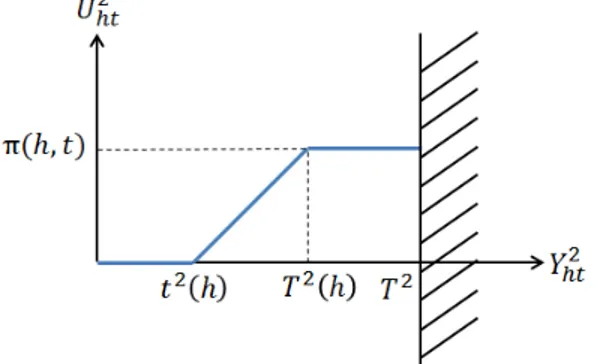
b) Heater System: A heater system is a background load for which we consider that power drawn can be reduced from its nominal value Pmax(h) to a minimal value Pmin(h).

The utility derived from the usage of this appliance depends on the temperature indoor, that we denote byY2

ht, and on users

presence or probability of presence, that we denote byπ(h, t) (see figure 2).

Fig. 2. Utility of space heater as a function of the indoor temperature

The 3 parameters indicated on the x-axis represent, respec-tively from left to right: the minimum acceptable temperature, the targeted temperature and the maximum acceptable temper-ature.

Temperature evolution dynamics are modeled by the fol-lowing equation:

Y2

ht= Yh2(t−1)+ A(h)Xht2 + B(h)(T0(t) − Yh2(t−1)) where

Y2

htis the temperature in homeh at time t, A(h) and B(h) are

coefficients for heating and insulation in homeh and T0_{(t) is}

the exterior temperature at time t.

IV. STUDIED SYSTEM AND CORRESPONDINGMODEL

In this section we first introduce the specific system we study by making some assumptions on the general system proposed in Section III-B. Then, we present the model we define for this specific system in order to evaluate and compare the performances of the different control approaches introduced in Section III-C.

A. System Assumptions

We focus on the functional groups introduced in Section III-B and we make the following assumptions:

• The system has no storage capabilities (neither at DSO/aggregator infrastructure nor at user premises). • Power losses introduced by the distribution network

are considered similar for all the users and hence the location of a user doesn’t affect the decisions related to his power share.

• The decision elementDEa knows the available

gen-eration capacity as a function of time.

• Only non critical loads are considered; capacity is supposed to be large enough to accommodate all critical demands. Available capacity therefore denotes remaining capacity after power has been allocated to all critical loads.

• Required exogenous information is known (either only byDEuor by bothDEu andDEa depending on the

analyzed control scheme).

• The state of the appliances that are part of the system, their electric characteristics and the values of relevant variables (e.g. temperature at a home) at the beginning of the crisis are known (either only byDEuor by both

DEu and DEa depending on the analyzed control

scheme).

• For the control schemes where DEa works at a

user granularity, DEa is configured with the set of

maximum power level each user has subscribed to. • Time is slotted and the power consumed by an

appli-ance is supposed to be constant in a time slot. Technologies for deploying autonomic capabilities forDEuto

self-discover part of the required data are today mature.

B. Model

The target of the system is to offer the highest possible quality of experience while complying with system capacity constraintsC(t) for all time instants t.

Next, we present a set of optimization problems that expresses the previous sentence and the system constraints in a formal language for each of the control schemes we have introduced. We denote by T the duration of the starvation period in number of time slots, byH the number of homes and byA the number of appliances per home. Table I summarizes the notation we use.

System Parameters and Exogeneous Variables

τ Duration of a time slot

C(t) Available power capacity at time slot t pa

(h) Minimum power consumed by appliance a in home h Pa

(h) Maximum power consumed by appliance a in home h π(h, t) Expected value of presence in home h at time t t2

(h) Minimum acceptable indoor temperature for home h T2

(h) Preferred indoor temperature for home h T2

Maximum acceptable indoor temperature T0(h) Initial indoor temperature for home h

A(h), B(h) Coefficients for temperature dynamics in home h T0

(t) Outside temperature at time t Ci

(h) Power limits for home h in increasing order

Control Variables and Controlled Variables

Ua

ht Utility of appliance a in home h at time t

Xa

ht Power consumed by appliance a in home h at time t

xa

ht = 1 when appliance a in home h at time t is active and

= 0 otherwise Y2

ht Temperature of home h at time t (continuous)

y2

ht Equals0 when temperature of home h at time t is less

than or equal to t2(h) and 1 otherwise Lht Power limit for home h at time slot t (continuous)

zhti Equals 1 when power limit is equal to C i

(h) and 0 otherwise

c) Global Maximum Utility, ahead of time: maxXa ht,x a ht PT t=1 PH h=1 PA a=1Uhta (1a) s.t. PH h=1 PA a=1Xhta ≤ C(t), ∀ t (1b) pa_(h)xa ht≤ Xhta ≤ Pa(h)xaht, ∀ t, ∀ h, ∀ a (1c) xa ht binary (1d)

Through the binary variable xa

ht (see Table 1), Equation

(1c) indicates that the power assigned to appliancea is either 0, either bounded between minimum and maximum. This excludes allocating a positive amount of power lower the the minimum; indeed, for some appliances, receiving less than the minimum possible power not only provides no utility but also can create some damage.

Please remark that the utility functions may depend on the dynamics of different variables, as introduced in Section III-D2), and therefore power allocations at one time slot will impact the utility in future time slots.

d) Global Maximum Utility, real time: Although the decisions are taken here per time slot, the dynamics of the system are still considered. For example, we don’t suppose an independent temperature measure at each time slot but tem-perature is calculated based on the modeled temtem-perature dy-namics, exogeneous variables and previously taken decisions. This enables to compare the performances of this scheme with those of the previous one. Indeed, although designed for usage in real-time, this scheme can also be used ahead of time, as it reduces the computation time and therefore increases scalability compared with the previous one (of course, such approach will lead to poorer performances). The constraints are the same as in the previous case and we have now T problems to solve consecutively:

max H X h=1 A X a=1 Uhta f or t = 1..T (2)

e) Global Maximum Utility under fairness constraints:

We present the ahead of time case; from which it is trivial to derive the real-time one.

The following problem computes the domain of the vari-ables where the minimum of the users utility is maximized.

maxXa ht,x a ht U (3a) s.t. PT t=1 PA a=1Uhta ≥ U, ∀ h (3b) PH h=1 PA a=1Xhta ≤ C(t), ∀ t (3c) pa_(h)xa ht≤ Xhta ≤ Pa(h)xaht, ∀ t, ∀ h, ∀ a (3d) xa ht binary (3e)

Let’s denote buyUM _{the solution of the previous problem.}

The following problem maximizes the global utility inside the domain computed by the previous one.

maxXa ht,x a ht PT t=1 PH h=1 PA a=1Uhta s.t. (4a) s.t. PH h=1 PA a=1Xhta ≤ C(t), ∀ t (4b) pa_(h)xa ht≤ Xhta ≤ Pa(h)xaht, ∀ t, ∀ h, ∀ a (4c) PT t=1 PA a=1Uhta ≥ UM, ∀ h (4d) xa ht binary (4e)

1) Local maximum utility under homogeneous capacity constraints: For this control scheme, the optimization problem is divided into 2 steps. First DEa decides the capacity to be

allocated to each user and then, at each user,DEudecides the

corresponding allocation per appliance by solving the M U

problem with H = 1. DEa takes decisions based on the

outcome of the following problem. For simplicity we present it for 2 levels of possible positive allocated capacities, but it is straight forward to generalize toM levels.

Lets denote byK the number of classes, by gkthe number

of houses in class k and by C2_{(k) the maximum power}

subscribed by users of class k. The power allocated to each home of class k by DEa equals C(t)C

2

(k) P

kgk.C2(k).

2) Rolling Black-Outs: The only difference between this

scheme and the previous one is the way DEa computes

the power it allocates to users. In this scheme, houses are ordered randomly. DEa allocates to each house either 0 or

the maximum subscribed power. During the first two hours, the first users in the list are served. Then the users are disconnected and the available power is provided for the next two hours to the next users in the list. DEa iterates this process and once

all users are served, it starts again from the beginning of the list and continues until the end of the optimization period T .

V. NUMERICAL ANALYSIS

A. Analyzed System

In this section we fix several system parameters and exoge-nous variables and we focus on the behavior of the presented control schemes as a function of the available capacity.

• We select a slot duration of τ = 5 minutes

• We consider a starvation period of 15 hours, so T = 180 slots.

• We suppose that the total available power during the

starvation period is constant, C(t) = C and we

analyze the model for different values of C.

• H = 50 houses are considered for two cases: homoge-neous and heterogehomoge-neous. For the heterogehomoge-neous case we suppose two classes of 25 houses each.

• We consider two types of appliances, A = 2, which

are lighting (index a = 1) and heating (index a = 2). We use the corresponding utility functions defined in Section III-D2. For lighting, we consider a particular case where the utility function is linear between p1

(Pmin) and P1 (Pmax). The rest of the curve is

• For all cases we suppose that the external and pre-ferred temperatures are supposed constant and equal, respectively,T0_{(t) = 10}◦_{C ∀t and T}2_{(h) = 20}◦_{C ∀h}

• We suppose that the expected value of the number of persons in the houses is constant during the whole studied period and we assume that both types of appliances are of equal importance for users. We therefore work with the normalized utility functions. The numerical analysis of the various presented mixed integer linear problems has been carried out using ILOG CPLEX Interactive Optimizer. Additional constraints have been introduced to the optimization problems to make them tractable in terms of time, without impacting the results.

B. Numerical results

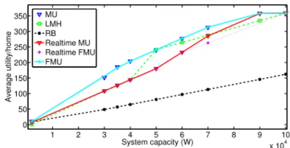
Since it is based on direct control and the largest set of data, schemeM U provides the maximum total utility over the optimization horizon. We therefore take it as the benchmark to compare all the schemes. Figure 3 shows the results for the homogeneous case with the following minimum and maximum accepted power for each appliance (in Watts): Lighting system [50, 1000], Heater system [1000, 4000].

Please observe that for facilitating the analysis we represent the total utility divided by the number of houses,

which means that the absolute gain of the M U scheme

compared with the others is 50 times larger than what is shown in the figures. Since utilities have been normalized per appliances (see Section III-D2), the maximum utility per slot equals 2 and therefore the total maximum utility per user equals 360. Performance is expressed by the average utility it provides to homes over the whole optimization period. The extreme left and right points on the x-axis correspond to the power values at which, respectively, the total utility for the LM H scheme reaches zero and the total utility for the M U scheme reaches the maximum possible utility.

Only the points in the graphs have been computed, the lines have been drawn facilitate reading.

As expected, the gain of all schemes is important compared to theRB scheme, except under very hard crises when scheme LM H fails at providing any utility.

The gains for schemes M U and F M U are significant, at least at certain levels of starvation, which may justify introducing the complexity induced by fine-grained control.

Scheme LM H reaches the performances of Scheme M U

for two specific values of the available capacity. The first one corresponds to the minimum power that can be allocated to the heating system of a given house (1000W). The fact that at this point, for Scheme LM H, all Heating Systems may be activated at certain times slots (even if not necessary at the same time slots) explains the rapid increase of the total utility at this specific total available capacity. The second one is trivial, it corresponds to the point where the capacity is enough to absorb the maximum possible demand.

The performances of Scheme LM H do not reach those

of Scheme M U in all cases. As an example, we consider the

1 2 3 4 5 6 7 8 9 10 x 104 0 50 100 150 200 250 300 350 System capacity (W) Average utility/home MU LMH RB Realtime MU Realtime FMU FMU

Fig. 3. Average utility perceived per user for different values of the capacity considering homogeneous homes

0 2 4 6 8 10 x 104 0 100 200 300 400 System capacity (W) Average utility/home MU LMH Realtime MU RB FMU Realtime FMU

Fig. 4. Average utility perceived per user for different values of the capacity considering heterogeneous homes

results presented in Figure 4 corresponding to a heterogeneous case with two classes. The minimum and maximum accepted power for each appliance (in Watts) are: Lighting system [50, 1000], Heater system [1000, 4000] for Class 1 and Lighting system [50, 500], Heater system [500, 2000] for Class 2.

Back to Figure 3, it is interesting to see that the real-time M U scheme significantly under performs scheme M U for most values ofC. This is explained by the fact that, since the approach has no vision on the future, DEa doesn’t allocate

enough power to the Heating system (it doesn’t predict the utility that can be generated in the future). Therefore, for low values of C, even when it can allocate power for the Heating system of some houses, it prefers to allocate the whole power to the Lighting system. On the contrary of the scheme LM H , the real-timeM U scheme can provide power to the Heating systems of some houses for values ofC smaller than 50000W, but as it has been designed, it decides not to do it. This shows that the real-timeM U mechanism is not well designed and that additional intelligence is needed when a real-time approach is required.

Figure 3 shows that in the homogeneous case, for this particular configuration, introducing fairness do not affect the total utility (F M U and M U have the same performances). This is not always the case, as shown in Figure 4 for the heterogeneous case.

VI. CONCLUSION

We propose a general approach for demand response solu-tions based on the possibility of extending visibility and control to users’ premises, and more precisely, having the capability to gather relevant information on existing appliances, to monitor relevant variables at users’ premises and to control individual appliances. These capabilities enable DSOs and aggregators

to evaluate the utility for end users of the allocated power. The possibility to take into consideration the evaluation of this utility enables new service and business models.

In order to leverage the above-listed capabilities, it is nec-essary to relate the targeted behavior of the controlled system with the services it provides. To cope with this requirement, we have proposed a taxonomy of appliances and a related approach for defining the utility of any king of appliances, as perceived by the users, as a function of the gathered information.

We propose and analyze a set of control schemes tending to maximize the total users utility under system technical and non-technical constraints (e.g. fairness constrains and constrains on data dissemination due to privacy issues). We consider ahead of time and real-time control schemes.

The analysis shows the high value of demand response mechanisms acting at fine granularity (e.g. per appliance visibility and control), specially when the period of power starvation is known ahead of time. We consider two cases in order to cover two different service models: in the first one a service provider takes control on the whole system (on individual appliances), in the second one, control is split in such a way that no sensitive data will be disclosed out of the houses and no control on local appliances will be delegated to an external entity. For both cases the proposed ahead of time mechanisms performances seems to justify the complexity induced by the fine-grained approach. A technical analysis to estimate the costs of an implementable solution is under development in the context of a joint program between EDF and Telecom ParisTech (Seido Lab).

When the starvation periods are not known ahead of time, the control mechanisms we propose act in a per slot basis; they keep traces of the past through the dynamics of the system, but have no view on the future, which induces poor performances. Such control schemes are not able to predict that allocating power at present time to a given appliance (e.g. Heater system) will create value in the future. For these schemes, additional intelligence has to be added to the system, which is a topic for further study.

Finally, we plan to combine the potentiality of the studied approach with a separate work we are carrying on possible participation of users to specific energy markets.

REFERENCES

[1] A. Agnetis, G. Dellino, G. De Pascale, G. Innocenti, M. Pranzo, and A. Vicino. Optimization models for consumer flexibility aggregation in smart grids: The address approach. IEEE First International Workshop

on Smart Grid Modeling and Simulation (SGMS), pages 96–101, 2011. [2] T. Bapat, N. Sengupta, S. K. Ghai, V. Arya, Y. B. Shrinivasan, and D. Seetharam. User-sensitive scheduling of home appliances. Proc.

2nd ACM SIGCOMM workshop on Green networking, 2011. [3] N. Gatsis and G. B. Giannakis. Cooperative multi-residence demand

response scheduling. 45th Annual Conference on Information Sciences

and Systems (CISS), pages 1–6, 2011.

[4] C. Joe-Wong, S. Sen, S. Ha, and M. Chiang. Optimized day-ahead pricing for smart grids with device-specific scheduling flexibility. IEEE

Journal on Selected Areas in Communications, 30(6):1075–1085, 2012.

[5] G. Karmakar, A. Kabra, and K. Ramamritham. Coordinated schedul-ing of thermostatically controlled realtime systems under peak power constraint. IEEE 19th RealTime and Embedded Technology and

Appli-cations Symposium (RTAS), 2013.

[6] D. Kofman and C. Rosenberg. New service models for electricity distri-bution during energy crises. Technical report. http://service.tsi.telecom-paristech.fr/cgi-bin/valipub download.cgi?dId=265.

[7] N. Li, L. Chen, and S. H. Low. Optimal demand response based on utility maximization in power networks. IEEE Power and Energy

Society General Meeting, 2011.

[8] J. L. Mathieu, M. Kamgarpour, J. Lygeros, and D. S. Callaway. Energy arbitrage with thermostatically controlled loads. European Control Conference (ECC), 2013.

[9] A. Mohsenian-Rad, V. W. Wong, J. Jatskevich, R. Schober, and A. Leon-Garcia. Autonomous demand-side management based on game-theoretic energy consumption scheduling for the future smart grid.

IEEE Transactions on Smart Grid, 1(3):320–331, 2010.

[10] A. Molderink, V. Bakker, M. G. Bosman, J. L. Hurink, and G. J. Smit. Management and control of domestic smart grid technology. IEEE Transactions on Smart Grid, 1(2):109–119, 2010.

[11] A. Nayyar, J. Taylor, A. Subramanian, K. Poolla, and P. Varaiya. Aggregate flexibility of a collection of loads π. IEEE Conference on

Decision and Control, 2013.

[12] P. Samadi, A.-H. Mohsenian-Rad, R. Schober, V. W. Wong, and J. Jatskevich. Optimal real-time pricing algorithm based on utility maximization for smart grid. First IEEE International Conference on

Smart Grid Communications (SmartGridComm), pages 415–420, 2010. [13] B. M. Sanandaji, H. Hao, K. Poolla, and T. L. Vincent. Improved battery models of an aggregation of thermostatically controlled loads for frequency regulation. arXiv preprint arXiv:1310.1693, 2013. [14] P. Srikantha, S. Keshav, and C. Rosenberg. Distributed control for

re-ducing carbon footprint in the residential sector. IEEE Smartgridcomm, 2012.

[15] P. Srikantha, C. Rosenberg, and S. Keshav. An analysis of peak demand reductions due to elasticity of domestic appliances. Proc. 3rd

International Conference on Future Energy Systems: Where Energy, Computing and Communication Meet, page 28, 2012.