Adaptive control, wide speed range flight and deconfliction

HAL Id: hal-01021535

https://hal-enac.archives-ouvertes.fr/hal-01021535

HAL is a multi-disciplinary open access archive for the deposit and dissemination of sci-entific research documents, whether they are pub-lished or not. The documents may come from

L’archive ouverte pluridisciplinaire HAL, est destinée au dépôt et à la diffusion de documents scientifiques de niveau recherche, publiés ou non, émanant des établissements d’enseignement et de

Adaptive control, wide speed range flight and

deconfliction

Catherine Ronflé-Nadaud

To cite this version:

Catherine Ronflé-Nadaud. Adaptive control, wide speed range flight and deconfliction. 2009. �hal-01021535�

Adaptive Control, Wide Speed Range Flight

and Deconfliction

AOARD-08-4128

AOARD-08-4130

Final Report

´

Ecole Nationale de l’Aviation Civile, Toulouse, France

Martin M¨

uller Engineering, Hildesheim, Germany

Report Documentation Page

Public reporting burden for the collection of information is estimated to average 1 hour per response, including the time for reviewing instructions, searching existing data sources, gathering and maintaining the data needed, and completing and reviewing the collection of information. Send comments regarding this burden estimate or any other aspect of this collection of information, including suggestions for reducing this burden, to Washington Headquarters Services, Directorate for Information Operations and Reports, 1215 Jefferson Davis Highway, Suite 1204, Arlington VA 22202-4302. Respondents should be aware that notwithstanding any other provision of law, no person shall be subject to a penalty for failing to comply with a collection of information if it does not display a currently valid OMB control number.

1. REPORT DATE 29 DEC 2009 2. REPORT TYPE FInal 3. DATES COVERED 01-09-2008 to 31-08-2009

4. TITLE AND SUBTITLE

Adaptive control, wide speed range flight, and deconfliction

5a. CONTRACT NUMBER

FA23860814130

5b. GRANT NUMBER

5c. PROGRAM ELEMENT NUMBER 6. AUTHOR(S)

Catherine Ronfle-Nadaud

5d. PROJECT NUMBER 5e. TASK NUMBER 5f. WORK UNIT NUMBER 7. PERFORMING ORGANIZATION NAME(S) AND ADDRESS(ES)

French Civil Aviation School,7, avenue Edouard Belin,Toulouse 31400,France,FR,31400

8. PERFORMING ORGANIZATION REPORT NUMBER

N/A

9. SPONSORING/MONITORING AGENCY NAME(S) AND ADDRESS(ES)

AOARD, UNIT 45002, APO, AP, 96337-5002

10. SPONSOR/MONITOR’S ACRONYM(S) AOARD 11. SPONSOR/MONITOR’S REPORT NUMBER(S) AOARD-084130 12. DISTRIBUTION/AVAILABILITY STATEMENT

Approved for public release; distribution unlimited

13. SUPPLEMENTARY NOTES

This research is funded by DARPA and US Army?s ITC-PAC. AOARD is the COR and the technical program manger is with ITC-PAC.

14. ABSTRACT

First part is dedicated to the "Adaptive Control". In the previous document, state of the art was reported and theoretical basis were assumed. Here, the simulation results and the real flight tests are detailed. Wind tunnel experiments have been carried out in order to provide accurate models and validate the theoretical process. Second part concerns the "Deconfliction". Two approaches are developed: Reactive Avoidance and Centralized Deconfliction. Both are illustrated and improved by simulations. In the third part entitled "Support", electronics improvements are presented as well as new vehicles manufacturing.

15. SUBJECT TERMS

Unmanned Aerial Vehicles, Control

16. SECURITY CLASSIFICATION OF: 17. LIMITATION OF ABSTRACT Same as Report (SAR) 18. NUMBER OF PAGES 35 19a. NAME OF RESPONSIBLE PERSON a. REPORT unclassified b. ABSTRACT unclassified c. THIS PAGE unclassified

Abstract

This paper is the final report for the ”Adaptive Control, Wide Speed Range Flight and Deconfliction” project.

First part is dedicated to the ”Adaptive Control”. In the previous doc-ument, state of the art was reported and theoretical basis were assumed. Here, the simulation results and the real flight tests are detailled. Wind tun-nel experiments have been carried out in order to provide accurate models and validate the theoretical process.

Second part concerns the ”Deconfliction”. Two approaches are developed: Reactive Avoidance and Centralized Deconfliction. Both are illustrated and improved by simulations.

In the third part entitled ”Support”, electronics improvements are pre-sented as well as new vehicles manufacturing.

As a conclusion, the project status is reported, next steps are considered, forthcoming tasks are listed and the agenda of the whole project is given.

Contents

4 Project Status and Planning 31 4.1 Project Status . . . 31

Chapter 1

Adaptive Control

1.1

Trajectories

When using fast adaptive control mechanisms, special care must be taken for the generation of reference trajectories.

Those 4D (temporal and spatial) trajectories reflect goals imposed by the user. In some cases those goals underconstrain the trajectories and the remaining degres of freedom can be used to optimize secondary objectives such as power consumption, control effort, etc... In other case, those goals overspecify the trajectory and it is desirable to be able to infer a set of degraded but fulfillable goals.

Some of the constraints on the trajectories are imposed by the vehicle performances, while others are the consequences of limits of the estimation or control algorithms. For instance, when using adaptation scheme of type MRAC, one has to be sure that the dynamic imposed by the trajectory stays within the bondaries imposed by the model. Failure to do so could lead to destabilization of the adaptation mechanism.

It is posible up to a certain extend to generate the trajectories off line. However, uncertainties due for example to environment (wind, turbulence, . . . ) or to variations in vehicle’s performances make it mandatory to be able to adapt the trajectories on the fly.

1.1.1

Impacts on Adaptive Control

Different trajectories will more or less stimulate the adaptation mechanism. Depending on the confidence in the quality of the estimated adaptation pa-rameters, it can be useful to dedicate available degrees of freedom or even infer degraded goals in order to enrich the trajectory with information favor-ing the operation of the adaptation mechanism.

In order to give an intuition of the forementioned phenomenon, we can use the following example: The autopilot of an aircraft is equiped with an adaptation mechanism intended to correlate roll rotational acceleration with deflection of ailerons in order to account for example for a variation of mass or of geometry. The goals given by the user is to fly between two waypoints, possibly optimizing travel time or energy consumption, so likely flying a straight line between those points. In normal conditions, atmospheric turbu-lences will force the autopilot to constantly level the wings, thus providing information for the adaptation mechanism to converge. In a very calm at-mosphere, the perturbations may not be sufficient for the corrections of the autopilot to provide a satisfactory convergence of the adaptation mechanism. In this case, it is interesting to degrade the travel time or energy consump-tion objectives and have the vehicle periodicaly perform some maneuvers to ensure the convergence of the estimation mechanism.

It thus appears important to have an estimation of the quality of the estimation of the adaptation parameters in order to be able to adapt the trajectory. The family of estimation agorithms known as Kalman filters naturaly provide such a feature in the form of the covariance matrix and seems thus especialy suited for that purpose.

1.1.2

Mathematics for the Generation of Trajectories

In order to respect physical laws, trajectories have to be smooth vector fields, at least twice continuously time derivable. It is often desired that those vector fields are more than twice continuously time derivable, in order to be able to compute nominal control vector for example when using properties related to differential flatness.

The generation of trajectories consists then in generating such vector fields, fulfilling a number of constraints and optimizing a number of criterion.

In order to do so, it is natural to seek a base of the Cn

functions. This base should have good properties to be able to deal with constraints and numericaly efficient in order to allow for real time computation.

The mathematical tools available to us can be sorted in two big families: polynomial and exponential functions.

1.2

Simulation

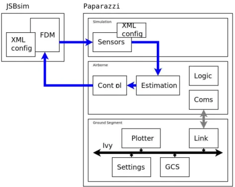
The simulation phase is an essential part of any control system design. In order to be useful, simulations must contain a physical model of the system and its sensors, so that both control and estimation algorithms can be tested

at the same time. Our objective was thus to have one simulator capable of handling various types of vehicles, with different dynamic characteristics, in a relatively easy manner. The “physical” simulation code is linked with the embedded code from the auto-pilot to run simulation cases. Previously in Paparazzi, this was done separately for each vehicle of interest, which required considerable code work each time a new vehicle or a new model of an existing vehicle became available.

We refer to this simulation framework composed of the complete Pa-parazzi suite augmented with the flight dynamic component of JSBsim as NPS: the New Paparazzi Simulator.

The JSBSim flight dynamics simulator1_{was chosen as the dynamic}

sim-ulation. It is an open source, multi-platform simulator, with a fairly wide range of tools, which allow the user to accurately simulate airframes of very different nature (airplanes, helicopters and rockets). JSBSim can be linked with crosscompiled control and estimation codes from the autopilot. In NPS it is linked to the Paparazzi suite in order to obtain a modular structure of the whole simulator, useful for debugging and analyzing results. Compared to a matlab like high level simulation, the cross compilation of the embedded autopilot code enables to test not only the theoritical validity of the algo-rithms but also their implementation. By being open source, JSBSim code can be modified to fulfill our specific needs when they exceed the scope of JSBsim’s parametrization.

The integration of JSBSim into the Paparazzi framework allows to run the simulator as a part of the whole system, using Paparazzi tools to monitor and record all flight parameters as well as to adjust control parameters.

Only the flight dynamic component from JSBsim is used. We use our own sensor model and cross compile the embedded code

1.2.1

JSBSIM FDM

JSBSim uses a coefficient build-up method for modeling the aerodynamic characteristics of aircraft. Any number of forces and moments (or none at all) can be defined for each of the axes. Each force/moment specification includes a definition comment, and a specification of the function that calculates the force or moment. The function definition can be a simple value, or a complicated function that includes trigonometric and logarithmic functions, and a one-, two-, or three-dimensional table lookup

Figure 1.1: Overview of NPS architecture.

As JSBsim is a widely used tool by an audiance ranging from advanced aerospace engineering students to industry professionals, numerous ready made FDMs are available for a number of unmanned aerial vehicles.

To create models of a specific vehicle, several tools are available, like DATCOM ( http://webstu.db.erau.edu/ mohamb5d/datcom/ ) which allow to infer aerodynamic and stability coefficients from a geometric description of the aerodynamic.

However JSBsim and those tools were developed mainly for full scale aircrafts aerodynamics. Being open source, JSBsim offers the possibility to write our own code for handling aspects specific to micro aerial vehicle aerodyamics. We had to resort to this option in developing NPS in order to provide a better suited model of a rotor for our quadrotor vehicle.

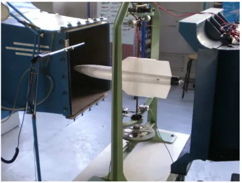
Jsbsim offers a good macroscopic description of a rotor behaviour. How-ever during flight tests on our quadrotor vehicle, we witnessed effects such as autopitching that was not predicted by this model and that adversely influenced our control. A finer analysis of the fluid mechanics around the rotor allowed us to derive a set of equations exibiting the witnessed effects. We were able to extend jsbsim by writing C++ code implementing this set of more accurate fluid mechanic equations. We then had to ressort to wind tunnel measurements to identifiy the coefficients involved in those equations.

Figure 1.2: wind tunnel experiment for propulsion

1.2.2

Cross Compilation

Cross compilation consists in compiling the exact same code that runs on the embedded system in the simulation framework. This is the solution that was chosen for NPS.

Compared to a matlab-like high level simulation where the algorithm is re-implemented, the cross compilation of the embedded autopilot code enables to test not only the theoritical validity of the algorithm but also its implementation.

In developing MAV, a strong constraint lies in the processing power capa-bilities. It is thus necessary to optimize the numerical representation of each variable of the control and estimation algorithms. A insufficiently accurate numerical representation of a variable or even of one calculation step will impair the efficiency of the algorithm and may remain unoticed due to the complexity of the whole chain. In a high level matlab type simulation, this aspect of the algorithm, purely related to implementation is seldom repre-sented. Comparison of the results produced by high level simulation used in prototyping the algorithm and NPS complete simulation allows to pinpoint such issues.

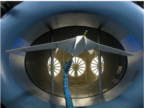
Figure 1.3: wind tunnel experiment for aerodynamic coefficients

However the transposition of the results obtained in simulation remains directly dependant on the relevance of the flight dynamic model and sensor model. In order to assess the validity of models and identify their coeffi-cient, a test bench is a must which allows to run experiments in a controlled environment as well as to use accurate sensors not compatible with real flight.

1.3

Test Bench

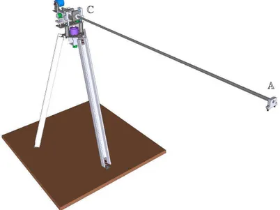
Experiments with vehicles, when performed outdoors, are subject to numer-ous perturbation sources (wind, turbulence, etc) for allowing a fair compari-son with simulation. When developing a control system, it is desirable to be able to separate the effects of each part of the system (measurement, esti-mation, control, adaptation) in order to quickly identify issues, their sources and their reasons. The latter cannot be done in real flight tests, where there are far too many degrees of freedom to cope with. Neither the simulation experiments can be completely trusted, given their limitations. This moti-vates the use of a test bench. Having a vehicle in a controlled environment, with precise measurement instruments, we stand midway between simula-tion results and real flight, which allows us to check performances of both estimation filters code and control laws separately. We have designed a test bench called BETH (BEnch for Testing Helicopters) given its primary use for

testing quadrotors control schemes. Beth is composed of a long arm with the shape of a tube, which can a) turn around the vertical axis without bounds of angle or number of turns; b) point up an down, thus changing the height of its outward tip A; and c) spin around its own axis.

Figure 1.4: The BEnch for Testing Helicopters

Beth has been designed to identify model coefficients as well as to assess the quality of said modes.

An added benefit of Beth will be to allow our students to manipulate a system that is easier to model and operate than a real vehicle.

The mechanical realisation of Beth is completed and the current develop-ment stage involves the finalization of the electronics and reference sensors.

1.4

Flight Experiments

We present in this section some results involving an adaptive behavior of the control. Several flight experiments have been conducted, dynamically modifying the airframe by dropping a part of a wing or/and dynamically changing the propulsion balance by cutting one of the two motors.

The flights have been conducted with a slightly modified airborne code which implements the theoretical results presented in the previous sections. This is presented in a preliminary section before detailing the flights.

1.4.1

Control Using Generation of Trajectories

In this section, the result of the control using the trajectory generation de-scribed in section 1.1 is presented. In the following graphs, the blue curves are the roll setpoints coming from the navigation control. The green curves are the output of the trajectory generation. We can see that the setpoint is smoothed and is now achievable by an aircraft. The curves are produced using JSBSim as flight dynamics simulator (see section 1.2) in order to model all the aerodynamic effects.

On figure 1.5, the control is only achieved by a simple proportional-derivative control. As a result, we have a static error between the measured roll angle and the reference trajectory.

Figure 1.5: Result of the trajectory generation (green) on the roll angle setpoint (blue). In red, the roll angle has static error and delay.

The static error can be removed by the use of an integrator in the control loop. The result is shown on figure 1.6. This type of control can also

compen-Figure 1.6: Effect of an integrator on the control. The static error is cor-rected, but delay and overshoot remain.

sate an asymmetry on the aerodynamics (see figure 1.10) or the propulsion (see figure 1.12).

However, a delay still remains because an error needs to be created before the proportional control has effect. This can be improved by adding a feed-forward control. It is possible thanks to the trajectory generation that can be derived two times. So, a gain is apply to the reference on acceleration, removing the delay as shown on figure 1.7.

Figure 1.7: Using a feedforward gain on acceleration remove the delay but an error still remains due to the damping effect.

Even with the feedforward gain, after a short time an error appears be-tween the achieved angle and its reference, especially in step command. This

comes from the damping effect of a drag proportional to the roll rate. To improve the control, this effect needs to be countered with an other feedfor-ward gain applied to the reference on rate. Figure 1.8 shows the result of the whole control loop with the trajectory generation, the two feedforward gains, the integral control and the classical feedback control.

Figure 1.8: A feedforward gain on the rate setpoint correct the error due to damping and overshoot is reduced too.

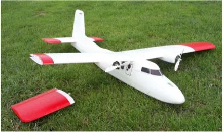
Figure 1.9: Aircraft used for wing-drop and motor-cut experiments.

1.4.2

Wing Drop

Flight experiments with a fixed wing aircraft were conducted to run the adaptive control software on board.

The first experiment was to remove a significant portion of the wing to unbalance the lift and drag to simulate a structural damage to the airframe. About one fifth of the right wing can be dropped by command from the ground. Around half of the aileron control surface at the edge are within this part of the wing and will be lost for control.

With the wing dropped the aircraft is still controllable by an experienced RC pilot in manual flight mode. The rudder is then used with a constant offset by the pilot to keep control over the aircraft. The aircraft tends to tilt over the right side and to tailspin when flown in sharp right turns.

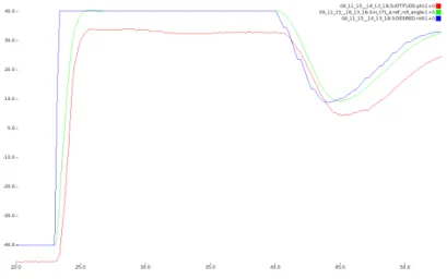
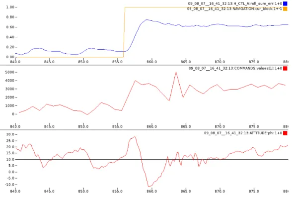
Plots given in figure 1.10 detail some measurements done in flight. On the top plot, the drop is materialized with the yellow curve which shows the block transition in the flight plan. On the same plot is displayed the adaptation parameter of the controler. It shows that the adaptation is achieved in a few seconds.

The middle plot shows the resulting roll command. It should be null to fly straight on a balanced aircraft while the maximum command is 10000. We observe that the missing wing part requires 40% of the command to stabilize the aircraft.

The bottom plot of figure 1.10 displays the roll estimation (measured from the infrared sensors). The oscillations before the drop show that the control is far from being perfect ! (even if the resulting trajectory is satisfactory, c.f.

Figure 1.10: Control behavior during a wing drop (t = 856). Top: Adapta-tion parameter. Middle: Roll command. Bottom: Resulting roll.

figure 1.11). On the wing drop, the aircraft banks to the right (due to the loss of lift on the right wing), up to 30 degrees. Then, the adaptation makes it banking slightly to the left (10 degrees) to come back to the track before stabilizing it.

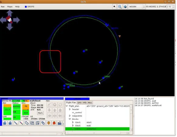
The figure 1.11 is the screenshot of the GCS some time after the drop (actually during a replay of the flight). The region where the drop occurred is squared in red. We see that it is hard to notice and the error is almost hidden in the noise !

1.4.3

Right Motor Cut

To even decrease the symmetry of the test aircraft one engine of the two engined aircraft can be turned on and off by command. The right motor is cut to simulate a heavy defect on the right wing side. In manual mode the aircraft can still be flown by the pilot but not landed as the controls are at its limits.

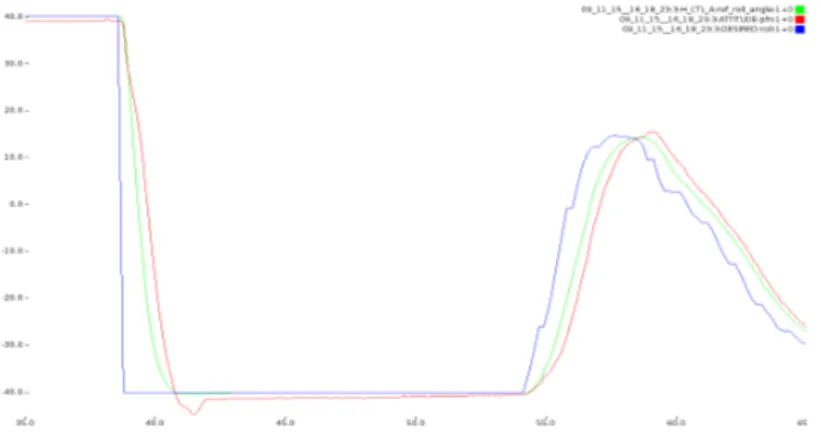
Figure 1.12 give extensive results for a flight where the motor was cut and the wing tip was dropped. The top plot shows the motors commands,

Figure 1.11: Achieved track during a wing drop. The almost perfect circle track is slightly bended during adaptation (in the red square).

Figure 1.12: Control behavior during right motor cut and wing drop (t = 510). Top: Left (red) and right (blue) motor commands. Middle: Adaptation parameter. Bottom: Roll command.

Figure 1.13: Achieved track during right motor cut. North west region: motor cut. East region: motor restarted.

the left one in red and the right one in blue which is cut when reduced to its minimum value (around 1000).

The adaptation roll parameter is displayed in the second plot (in red) and the resulting roll command in the bottom plot. We can observe a satisfactory response to the first motor cut around t = 450.

The drop command occurs around t = 510. Unfortunately, the release device did not properly and the wing tip stayed linked to the aircraft. We see that the adaptation fights against this modification, until t = 540. During the next 30s, the safety pilot shaked the aircraft in manual to actually get rid of the wing tip. Autonomous (auto2 in the Paparazzi vocabulary) control restart at t = 570. We observe that the adaptation parameter and the roll commands are not null to compensate the lost wing part. At t = 600, the right motor is cut and we see that the adaptation and the resulting roll command increase a lot. The command reaches almost 80% of its maximum to keep the plane stabilized. Lower values are reached when the motor is restored (t = 635).

1.4.4

Ongoing Experiments

Wide Speed Range Aircraft

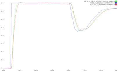
Figure 1.14 give some preliminary numbers about the achievable speed range of the new designed aircraft presented in chapter 3. The adaptive required control for this aircraft is in progress and no satisfactory results have been obtained yet.

Figure 1.14: Throttle (in %) and ground speed (in m/s) for a wide speed range aircraft.

Figure 1.15: Damage on the left wing due to a mid-air collision during test flights.

Unwanted Aircraft Modification

The test flights were done by flying large circles at a regular RC field. While changing parameters at the ground station the RC safety pilot noticed a glitch in the flight path and another aircraft nearby. The pilot of this other aircraft told that he might have hit our aircraft in flight but was not sure. The wing-drop aircraft was flying perfect so it was assumed that there was no collision. The other aircraft landed and had red color on the glass surface of its wing and that it was very likely that the aircraft were actually touching. When switching to manual mode for landing the RC pilot noticed that the aircraft was acting strange. The aircraft was immediately landed and it was observed that the aileron was cut and about half of it was bent upwards. This was not possible to see by looking at the flight envelope and showed the need for collision avoidance.

This story provides us the prefect transition to the next chapter about deconfliction!

Chapter 2

Deconfliction

We present in this chapter two experiments for achieving deconfliction, a reactive distributed solution and a centralized planned solution.

2.1

Reactive Avoidance

Figure 2.1: Repulsive forces to keep a safety distance between aircraft A and B. Applied F forces are orthogonal to the A − B segment with a norm computed from the relative velocity between the mobiles.

This approach for collision avoidance is based on potential fields:

• Aircraft communicate to each other their current position and velocity and they continuously perform a conflict detection;

• Virtual 3D repulsive forces are added between the aircraft (figure 2.1) based on position prediction if they are close enough;

• Corrections are applied on the heading and the altitude.

The figure 2.2 shows a simulation of three UAVs. Two of them (blue and green paths) are flying on the same circle in different directions. They compute the forces in order to avoid each other. We can see that the path of the two UAVs are modified at some points of the circle. The displacement is either vertical and horizontal as the forces are computed in 3D.

The last UAV (red path) arrives later and is flying on a small circle crossing the two other paths. This aircraft is an intruder, he has no avoidance mechanism but his position is known. So, the two other UAVs react to his presence by changing their heading and altitude.

Figure 2.2: Two UAVs (green and blue) are using potential fields in order to perform reactive collision avoidance; one UAV (red) is an intruder and doesn’t take other aircraft into account.

This solution shows some efficiency even in a small area with more than two aircraft and intruders. It is also fully distributed, light in computation time, react vertically and horizontally and doesn’t need information accept the state (position and speed) of the other aircraft. The main drawback is that their is no guarantee of collision avoidance. This approach should only be used as a last resort for escape maneuvers.

A TCAS-like1 _{solution, even if only vertical, could have better}

proper-ties than purely reactive approach. It can integrate a coordination protocol between the aircraft that can reduce the risk of corrections in the same di-rection, improving the reliability of this method.

2.2

Centralized Deconfliction

We have implemented a centralized deconfliction solution inside the Pa-parazzi System. We give in this section a description of the proposed solution and some preliminary results we got in simulation.

2.2.1

Centralized Conflict Solver for Paparazzi

Maneuvers

In this experiment, the deconflicter tries to find a solution in the horizontal plane. The allowed maneuver for collision avoidance is displayed in figure 2.3: the aircraft leaves it nominal track for a given time before coming back. This maneuver will be achieved using the “lateral shift” feature of Paparazzi: The pilot is allowed to ask the aircraft to shift to the right or the left of its nominal track. This order, usually given from the GCS interface, will be here sent by our deconflicter.

T0 T1

T2

α

Figure 2.3: Proposed horizontal maneuvers for the centralized deconflicter.

Architecture

Our deconflicter has been included in the Paparazzi distributed architecture as displayed in figure 2.4:

• This standalone agent listen for the aircraft status broadcasted by the server.

• The agent predicts the upcoming tracks and detects the potential con-flicts (distance between two aircraft less than a given separation) • The agent computes maneuvers for the in-conflict aircraft.

• The computed maneuvers are sent over the network and forwarded by the server (after logging) to the aircraft.

Aircraft

Sends telemetry messages Receives datalink messages

Aircraft

Sends telemetry messages Receives datalink messages

Ground network

telemetry ground ground ground

telemetry

datalink

telemetry ground link

Connects a hardware wireless device to the network

gcs

Displays graphic data Controls the datalink

server

Logs raw messages

Dispatches synthetic messages deconflicter

Wireless link

datalink

Airborne network

Send avoidance maneuvres

Figure 2.4: Centralized deconfliction architecture over the Ivy bus. The new agent receives the aircraft’s status from the server and send back avoidance maneuvers.

Trajectory Prediction

In the present solution, the flight plan of the aircraft is not taken into account and only the “radar” track is used. The observed status of the aircraft includes:

• The 2D position (the altitude is ignored); • The ground speed;

• The ground course;

• The first derivative of the ground course.

The current position is simply extrapolated with the speed, the course and its derivative. The latter is enough to do correct prediction over a circle. Note that the attitude of the aircraft is not used: It is not helpful if the wind is not known.

For our experiments, the prediction time is around 5s. For aircraft flying around 15m/s face to face, it means that the conflict is detected when the vehicles are 150m from each other.

Resolution

Maneuvers are computed for free aircraft. We call free, an aircraft which • is ready to accept a maneuver (i.e. is not an intruder);

• is not already executing a maneuver.

A maneuver is a right or left shift during a given time (6s for our experi-ments). Two values for the deviation are considered: 10 and 20m. All the possible maneuvers are evaluated simultaneously for all the free aircraft and the best one is chosen, trying to

• Solve all the conflicts;

• Maximize the distance between the in-conflict aircraft; • Minimize the sum of shifts.

Since we consider small problems (less than ten vehicles), the whole search space can be easily explored and an optimal solution can be found.

2.2.2

Results

The previously described solution allowed us to obtain some results for simple scenarios.

One of the difficulties is to build conflicts to solve; it is not so easy to get aircraft in the same place at the same time! To achieve this goal, we have asked the aircraft (through their flight plan) to follow a hippodrome figure (it is a built-in function in Paparazzi flight plan language) to get conflicts over straight lines and along curves.

In these first experiments, we have three aircraft circling over one single hippodrome:

• A fast yellow aircraft circling clockwise; • A slow blue aircraft circling clockwise; • A red aircraft circling clockwise.

Figure 2.5: Deconfliction for a face to face conflict.

Figure 2.5 displays the solution for a face to face conflict: The two aircraft shift their position (following their ”carrots”) to the left of the nominal track (the green straight lines). The plot shows here the middle of the maneuvers and the aircraft will start to come back on the original tracks.

Figure 2.6 displays the solution for overtakings along a curve and a line. For the circle, the overtaking yellow faster aircraft shifts its track by increas-ing the radius of the circle it is followincreas-ing. The overtakincreas-ing over a line here requires a shift to the right from the slow blue aircraft and a shift to the left from the fast yellow aircraft.

Figure 2.6: Deconfliction by overtaking.

Figure 2.7 shows a more complex situation where three aircraft are in-volved requiring two synchronized maneuvers. The red aircraft has just avoided the blue one along the circle by a shift to the right (increasing its circle radius) before coming back on the hippodrome. The yellow aircraft has turn to the left to leave the place to the red one and is now ready to overtake the much slower blue aircraft.

Chapter 3

Support

3.1

Flight Computer

Figure 3.1: Breadboard prototype of the new flight computer.

The work on deconfliction showed the need for high level sophisticated communications. This kind of communications are much easier to implement with the help of an operating system as code for hardware drivers and network stacks is readily available and well tested.

The work on adaptive control showed the need to have a massive pro-cessing power available. This allows to test non optimized algorithms using floating point numbers and readily available numerical libraries, like GNU GSL (Gnu Scientific Library) or OpenCv (Open Computer Vision) .

Even though the Linux kernel running on the Gumstix Overo can be op-timized to handle near real time tasks, those usually simple but fast tasks tend to put a lot of load on the CPU, by triggering numerous context switch-ing. High frequency and time critical processing such as sensors sampling or actuators driving are better handled in a OS less processor.

This led us naturally to design a twin processor solution combining the advantages of one OS less ARM Cortex M3 and a gumstix Overo featuring an OMAP35 running Linux.

The Cortex M3 is ideally suited to run all IO tasks while providing ample processing power to run control algorithms once they’ve been optimized. The OMAP35 running Linux offers the flexibility of this operating system’s extensive hardware drivers as well as gargantuan processing power for easy prototyping.

The communications between the two processors require both low latency, high throughput and low overhead. The following table summarizes the different peripherals available on both processors.

Description Bandwidth Remarks

I2C Synchronous, half duplex ≤400 Kbit/s

RS232 Asynchronous, full duplex ≤10 Mbit/s Easy support on both pro-cessors

SPI Synchronous, full duplex ≤230 Kbit/s Requires a kernel driver on the OS processor

USB Asynchronous, full duplex, Differential

1.5-12 Mbit/s Complex software stack on the OS less side

Figure 3.2: Pros and cons of possible hardware interfaces between the real-time micro-controller and the Linux processor

3.2

Vehicle

3.2.1

Structure Change

For the structural change flight experiments a well known good-natured high wing aircraft (Multiplex Twinstar II, see figure 1.9) was chosen. This aircraft is easy to fly in the standard configuration and often used as a beginners aircraft for RC pilots. The weight is about 1.5kg and the wingspan 140cm. The autopilot controls the elevator, ailerons and throttle. The manual pilot can also control the rudder.

To simulate a structural damage of the wing the outer 24cm of the right wing are dropped by command. About 50% of the aileron control surface are lost so that the control is also unsymmetrical. The dropable wing part is pushed into overlapping plastic sheets covering the rest of the wing and hold by a strong ’locking’ arm mounted on a RC servo in the wing center. This

Figure 3.3: Wing drop mechanism. The center servo locks the part in flight, the outer two servos push the wing when dropped.

servo has to carry a significant force and cope with the alternation of load. To release the wing the lock servo sets it free and two other servos push the wing away from the aircraft and the covering plastic sheets (see figure 3.3).

3.2.2

Wide Speed Range

The development started with a two engined aircraft (see figure 3.4) with a large diameter foldable propeller in front for slow flight and a small diameter propeller in the back for fast flight. The design was abandoned because the two motors increased the overall weight in a way that a slow flight was difficult to achieve and due to the fact that the small back propeller could not achieve a higher speed than the front propeller did. The ”hanging prop” maneuver was not possible with this type of wing shape so that it was decided to fly with a high angle of attack flight instead.

The new airframe (see figure 3.5) has the propeller in front to have air flow and force on the control surfaces even in slow flight. It was observed that the cancellation of torque through two counter-rotating motors was not needed for this aircraft. The propeller is no longer a ”slow flight” that has been designed for small electric planes but a type that is used on gas engine

Figure 3.4: Two propellers design aircraft.

aircraft. The airfoil is designed for fast flight. The wing geometry has been changed from delta to trapezoid to have a bigger surface for lift in slow flight. The prototype is made of glass covered Styrofoam. First test flight results can be found in 1.14. Currently the aircraft is redone as the flight characteristics were not as wanted. The control surfaces are too big and will be reduced in size.

Chapter 4

Project Status and Planning

We present in this chapter a summary of the actions we did during the last six month and future prospects for the second year.

4.1

Project Status

4.1.1

Adaptive Control

At the end of the first year of the project, the ”Simulation” task is completed. The simulator has already been used for quadrotors and fixed-wing aircraft. It is a new tool for the lab, useful to test and improve new prototypes before real flights. Simulations give us a lot of information on more and more complex dynamics.

Concerning the ”New aircraft use case” task, a push tail prototype has been designed, built and flown manually. Improvements are studied before the installation of the Paparazzi autopilot.

For the ”Structure change use case” and ”Payload change use case” tasks, as written in chapter 1, MME built a twinstar with a removable part of wing. Flight tests and automatic tuning were done in August.

Results are detailed in Chapter 1.

4.1.2

Deconfliction

Some scenarios described in the previous report, have been implemented and tested, as presented in chapter 2 :

• short term trajectory prevision; • centralized horizontal deconfliction;

• reactive behaviour for vertical deconfliction.

4.1.3

Next Steps

In the second year of the project, a new Work Package ”Wide Speed Range Flight” will be tackled. The goal of this work package is to explore possibili-ties to extend fixed-wing MAVs flight envelope in the low speed region. Two tasks are planned :

• Testing of new sensors to cope with augmentation of the flight envelope. Of course, the integration of sensors and antennas in the aircraft will be studied.

• Fligh tests with developed equipment for recuperation of flight data and improvement of obtained results.

Concerning the Work Package ”Deconfliction”, flight tests with more air-craft with varying characteristics (speed envelopes) will be done and scenarios described in the first report will be tested.

In order to be more friendly, a new HMI will be developed on the Ground Control Station. Then, we will have flight tests with this new HMI and the operator behaviours will be studied, in real conditions. This will help to improve and validate our choices.

In the Work Package ”Infrastructure”, Onboard Computation Environ-ment will be developed. In particular, we will improve Board-to-board com-munications. All these new developments will be tested during all the flight demonstrations.