Suivi par sonar de la dynamique des dépôts en réseau d'assainissement

HAL Id: hal-01712037

https://hal.archives-ouvertes.fr/hal-01712037

Submitted on 19 Feb 2018

HAL is a multi-disciplinary open access archive for the deposit and dissemination of sci-entific research documents, whether they are pub-lished or not. The documents may come from teaching and research institutions in France or abroad, or from public or private research centers.

L’archive ouverte pluridisciplinaire HAL, est destinée au dépôt et à la diffusion de documents scientifiques de niveau recherche, publiés ou non, émanant des établissements d’enseignement et de recherche français ou étrangers, des laboratoires publics ou privés.

d’assainissement

Iacopo Carnacina

To cite this version:

Iacopo Carnacina. Suivi par sonar de la dynamique des dépôts en réseau d’assainissement. [Research Report] IFSTTAR - Institut Français des Sciences et Technologies des Transports, de l’Aménagement et des Réseaux. 2011, 135p. �hal-01712037�

Projet VITRES 2009

CONVENTION POUR LE SOUTIEN FINANCIER DE

L”INSTITUT CARNOT VITRES - N° 07 CARN 013 01

S

UIVI PAR SONAR DE LA DYNAMIQUE DES

DEPOTS EN RESEAU D

’

ASSAINISSEMENT

Author: Iacopo Carnacina

SOMMAIRE LIST OF FIGURES ... 2 LIST OF TABLES ... 5 LIST OF SYMBOLS ... 6 1 INTRODUCTION ... 8 2 LITTERATURE REVIEW ... 9

2.1 Generic back ground and definitions ... 9

2.2 Sediment interface in combined sewer deposits ... 16

3 SONAR THEORETIAL BACKGROUND ... 18

4 EXPERIMENTAL APPARATUS ... 20

4.1 Marine Electrics 1512 SONAR ... 21

4.2 Sontek 10 Mhz side looking ADV ... 28

4.3 In-situ setup ... 30

5 EXPERIMENTAL SITES, EXPERIMENTAL SETUP AND MEASUREMENTS PROCEDURE. ... 33 5.1 Experimental sites ... 33 5.2 Measurement execution ... 38 5.3 Data elaboration ... 39 5.3.1 Profiler.m ... 40 5.3.2 ADVDATAELABORATION.M ... 47 6 RESULTS ... 51

6.2 Duchesse Anne (DA) tests ... 51

6.2.1 Morphological characteristics Test DA-S1 (2010-10-20) ... 51

6.2.2 Morphological characteristics Test DA-S5 (2011-05-11) ... 54

6.2.3 Temporal evolution Test DA-S4 (2011-05-11) ... 58

6.2.4 Flow filed Test DA-S2 (2011-01-21) ... 60

6.2.5 Flow filed Test DA-S3 (2011-02-04) ... 66

6.3 Allée de l’Erdre tests (AE) ... 73

6.3.1 Morphological characteristics Test AE-S6 (2011 03 10) ... 73

6.3.2 Morphological characteristics Test AE-S7 (2011 03 24) ... 77

6.3.3 Morphological characteristics Test AE-S8 (2011 05 04) ... 81

6.3.4 Temporal evolution Test AE-S5 (2011 02 09) ... 85

6.3.5 Temporal evolution Test AE-S9 (2011-06-16) ... 87

6.3.6 Flow field Test AE-S2 (2010-11-26) ... 95

6.3.7 Flow field Test AE-S3 (2010-12-15) ... 102

6.3.8 Flow field Test AE-S4 (2011-02-02) ... 115

6.4 Acoustic backscatter correlation with TSS ... 123

6.5 Comparison between velocity profiles ... 124

CONCLUSIONS ... 127

REFERENCES ... 128

LIST OF FIGURES

Figure 1 lutocline definition ... 9

Figure 2 Green et al 1999 definition ... 12

Figure 3 Sediment point gauge. The disc has a thickness of 2 cm and a diameter of 25 cm. .. 20

Figure 4 SONAR Marine Electronics model 1512. ... 22

Figure 5 pipe profiler SONAR output for PL= 4 us ... 24

Figure 6 pipe profiler system control panel. ... 25

Figure 7 detection algorithms proposed in the Marine Electronics Pipe Profiler software ... 28

Figure 8 ADV and SONAR fastening (same as in-situ conditions) ... 31

Figure 9 Reference system definition ... 32

Figure 10 catchments basins with pipes, quotes (in m) and working section locations ( ). Note: tick black lines are the combined sewer networks. ... 34

Figure 11 catchments basins invert sketch with notation (a) AE (b) DA (dimensions in meters). ... 35

Figure 12 Experimental in situ set-up ... 37

Figure 13 definition sketch of the ADV control volume position ... 39

Figure 14 Sonar output from laboratory experiences and insitu conditions. ... 41

Figure 15 section y=0, corresponding to θ=180° and j=200 ... 42

Figure 16 Sonar output before and after application of the filter ... 44

Figure 17 Matlab script example, data before filtration ... 45

Figure 18 Matlab script example, data filter analysis, blue line represents the median, red and green line represents the confidence bound of width σ. ... 46

Figure 19 Matlab script example, data after filtration ... 46

Figure 20 3D surface bottom surface generation after filter application; data have been displayed from the new reference system relative to the invert zBED. ... 47

Figure 21 quadrant analysis classification ... 49

Figure 22 Test DA-S1 in situ suspended solids concentrations and particle size distributions 51 Figure 23 Test DA- S1 output ... 54

Figure 24 Suspended solids concentration test DA-S5 with the free surface (solid line) ... 55

Figure 25 DA-S5 sediment morphology measured with the sonar, flow from left, the scale represents the zBED elevation in mm. ... 56

Figure 26 DA-S5 sediment morphology measured with the sonar from the average plane, flow from left, gray scale represents the zPLANE elevation in mm. ... 56

Figure 27 DA-S5 longitudinal profile for y=0m ... 57

Figure 28 DA-S5 Sonar output at section x=-3.20 m ... 58

Figure 29 Test DA-S4 in situ suspended solids concentrations and particle size distributions 59 Figure 30 Sediment interface temporal evolution detected for tests DA-S4 ... 60

Figure 31 Test DA-S2 in situ suspended solids concentrations and particle size distributions 60 Figure 32 (a) DA-S2 transverse profile at x=-0.5 m, and (b) amplitude profile at y=0 m ... 61

Figure 33 (a) DA-S2 transverse profile at x=-1.9 m, and (b) amplitude profile at y=0 m ... 61

Figure 34 Longitudinal survey referred from the channel sonar centre ... 62

Figure 35 centreline longitudinal profiles from the interpolating plane zPLANE ... 62

Figure 36 DA ADV data sect. 1 (x=-0.5 m) ... 63

Figure 37 DA ADV turbulence data sect. 1 (x=-0.5) ... 64

Figure 38 DA ADV data sect. 2 (x=-1.9 m) ... 65

Figure 39 DA ADV turbulence data sect. 2 (x=-1.4 m) ... 66

Figure 40 Test DA-S3 in situ suspended solids concentrations and particle size distributions 67 Figure 41 DA-S3 Bottom morphology ... 67

Figure 42 DA-S3 centerline longitudinal profile (y=0), where the regression line represents

the regression trough the zBED points. ... 67

Figure 43 DA-S3 ADV data sect. 1 (x=-0.5 m) ... 68

Figure 44 DA-S3 ADV turbulence data sect. 1 (x=-0.5 m) ... 69

Figure 45 DA-S3 ADV data sect. 2 (x=-1.9 m) ... 70

Figure 46 DA-S3 ADV turbulence data sect. 2 (x=-1.9 m) ... 71

Figure 47 DA-S3 ADV data sect. 2 (x=-3.3 m) ... 72

Figure 48 DA-S3 ADV turbulence data sect. 2 (x=-3.3 m) ... 73

Figure 49 TSS, VSS and particle size distribution conditions of test AE-S6 ... 74

Figure 50 AE-S6 sonar output at x=0 mm ... 75

Figure 51 AE-S6 Bottom morphology measured with the sonar profiler, from the invert zBED in [mm]. ... 76

Figure 52 AE-S6 Bottom morphology measured with the sonar profiler,from the interpolating plane zplane in [mm]. ... 77

Figure 53 AE-S6 longitudinal profile for y=0 m. ... 77

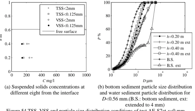
Figure 54 TSS, VSS and particle size distribution conditions of test AE-S7at x=0 mm ... 78

Figure 55 AE-S7 sonar output at x=0 mm ... 79

Figure 56 AE-S7 Bottom morphology measured with the sonar profiler, zBEDin [mm] ... 80

Figure 57 AE-S7 Bottom morphology measured with the sonar profiler, zPLANE in [mm] ... 81

Figure 58 AE-S7 longitudinal section y=0 m ... 81

Figure 59 TSS, VSS and particle size distribution conditions of test AE-S8 ... 82

Figure 60 Sediment deposits surveyed with a clear Perspex cylinder of 7 cm of internal diameter. ... 82

Figure 61AE-S8 sonar output at x=-0.30 mm ... 83

Figure 62 AE-S8 Bottom morphology measured with the sonar profiler from the invert bottom zBED in [mm] ... 84

Figure 63 AE-S8 Bottom morphology measured with the sonar profiler, zplane in [mm] ... 85

Figure 64 AE-S8 longitudinal section at y=0 mm. ... 85

Figure 65 TSS, VSS and particle size distribution conditions of test AE-S4 (2010-02-02) .... 86

Figure 66 AE-S5 Sonar output ... 86

Figure 67 AE-S5 Bottom morphology measured with the sonar profiler from the invert bottom zBED in [mm] ... 87

Figure 68 Flow depth, longitudinal flow velocity and rain intensity for the survey period ... 88

Figure 69 TSS, VSS and particle size distribution conditions of test AE-S7 ... 88

Figure 70 Test S9, Morphological survey, at 2:00, 7:00 and 10:00. Colour shading represents the z elevation in mm from the invert bottom ... 89

Figure 71 AE S9 sonar output at t=4:35 at x=-9900 mm, referred toward the SONAR center 90 Figure 72 AE S9 sonar output at t=10:00 at x=-9900 mm, referred toward the SONAR center ... 91

Figure 73 Test AE S9. Bottom morphology temporal survey interpolation (blue dots represent the actual surveyed data). Colour shading represents the z elevation in mm from the invert bottom. ... 92

Figure 74 Instantaneous longitudinal flow velocity and turbulences recorded during the morphological survey at section x=0 m. ... 95

Figure 75 TSS, VSS and particle size distribution conditions of test AE-S2 ... 96

Figure 76 AE S2 model set-up pipe profiler output. ... 96

Figure 77 AE–S2 data.output; the contour lines represent the 8 bit signal amplitude (coloured scale from 0 to 256 counts) observed by the sonar, ( ) gauge position. ... 97

Figure 78 section y=0 m, AE S2 data for pulse length of 4 µs, 8 µs, 12 µs, 16 µs and 20 µs (legend represents the range and pulse length). ... 98

Figure 79 AE S2 model results from the filtered ADV readings (of which generally more than 95 % were considered good): (a-c) V= velocity cm/s, (d-f) COR= signal correlation %, (g-i) SNR= sound to noise ratio, db, (l-n) AMP= backscattered signal amplitude of the control

volume, counts. Note: 0=beam 0, 1=beam 1, 2=beam 2 ... 99

Figure 80 AE S2 model results from the filtered ADV readings (of which generally more than 95 % were considered good): test over field sediments; variation toward the water column of the Reynolds stress. ... 100

Figure 81 AE S2 unfiltered data normalized turbulence characteristics ... 101

Figure 82 AE S2 filtered data (Whal 2003 algorithm) normalized turbulence characteristics u*=0.99 cm/s and δ=0.88 m. ... 102

Figure 83 TSS, VSS and particle size distribution conditions of test AE-S3 (2010-12-15) .. 103

Figure 84 AE transverse profile sonar output ... 104

Figure 85 Test AE-S3 bottom morphology ... 105

Figure 86 AE longitudinal profile at x= 0m, sonar output, flow from the right. ... 106

Figure 87 (a) AE transverse profile at x=-0.5m, ( ) gauge position, (×) TSS sampler positions, (b) vertical amplitude profile at x=-0.5 m. ... 106

Figure 88 AE sect.1 averaged ADV data. ... 108

Figure 89 AE sect.1 Reynolds stress ... 109

Figure 90 AE sect.1 normalised stresses. ... 110

Figure 91 AE transverse profile at section 3 (x=-2.5m), ... 110

Figure 92 AE x=-2.5 m averaged ADV data ... 112

Figure 93 AE sect.3 Reynolds stresses ... 113

Figure 94 AE transverse profile at section 5 (x=-4.5m), and amplitude profile at x=0 m ... 113

Figure 95 AE sect. 5 averaged ADV data ... 114

Figure 96 AE sect.5 Reynolds stresses ... 115

Figure 97 TSS, VSS and particle size distribution conditions of test AE-S4 (2010-02-02) .. 115

Figure 98 Sonar output for x=-0.5 (white spot) sediment interface detected with the gauge 116 Figure 99 Sonar output for x=-1.5, (white spot) sediment interface detected with the gauge 117 Figure 100 Sonar output for x=-2.5 (white spot) sediment interface detected with the gauge ... 118

Figure 101 sediment surface referred to the invert test AE-S4 ... 119

Figure 102 AE-S4 ADV data sect. 1 (x=-0.5 m) ... 120

Figure 103 AE-S4 ADV turbulence data sect. 1 (x=-0.5 m) ... 121

Figure 104 AE-S4 ADV data sect. 3 (x=-2.5 m) ... 122

Figure 105 AE-S4 ADV turbulence data sect. 3 (x=-2.5 m) ... 123

Figure 106 Correlation between TSS<2 mm and amplitude in counts ... 124

Figure 107 DA-S3 Normalised velocity profiles and shear stress profiles ... 125

Figure 108 AE-S2 Normalised velocity profiles and shear stress profiles ... 125

Figure 109 AE-S3 Normalised velocity profiles and shear stress profiles ... 126

LIST OF TABLES

Table 1 Definitions of sediment bed elevation from literature. ... 13

Table 2 script tasks (see also the annexes for the script layout) ... 44

Table 3 ADVDATAELABORATION output ... 49

Table 4 Flow velocity recorded before the morphological survey at the section x=0 m ... 54

Table 5 Flow velocities measured at section x=0 m ... 74

Table 6 AE-S7 longitudinal flow velocities ... 78

Table 7 Test AE-S8 measured velocities ... 83

Table 8 Suspended solids concentrations measured at different times ... 88

LIST OF SYMBOLS

The following symbols have been used in this work:

<u’iu’j> Reynolds stress [m2/s2]

AMP signal amplitude [counts]

as the diameter of the particles, [m]

Bs constant [-]

C particle weigth concentration [mg/l]

c speed of sound in the water [m/s]

C1 constant [dB]

Cb reference concentration [mg/l]

COR correlation [-]

D* non dymensnioal diameter [m]

Dxx diameter for which xx% in weight of settled material is finer [m]

E received strength [counts]

e the relative elasticity of the material [-]

Er received noise respectively [counts]

f0 emitted frequency [Hz]

fs sampling frequency [Hz]

g the gravitational acceleration [m/s2]

h distance from the sediment interface [m]

H quadrant analysis hole size [m/s]

k acoustic wave number [m-1]

Kc acoustic signal conversion factor [dB/counts]

ks roughness heigh [m]

kw total kinetic energy [m2/s2]

M particle voluulme concentration [l/l]

nb number of backscatters [-]

PL transmit pulse length [m],

PT transmit power [W],

R range along the beam axis [m],

s specific density [-]

S energy slope [-]

SNR signal to noise ratio [dB]

Sv scattered signal in decibel [dB]

Si,H single burst event contribution [-]

t time [s]

T the transport stage parameter [-]

TSS total suspended solids concentration [mg/l]

TT transducer temperature [°C],

U depth averaged flow velocity [m/s]

u average longitudinal flow velocity [m/s]

u instantaneous longitudinal flow velocity [m/s]

u* critical shear velocity [m/s]

u* shear velocity [m/s]

u’ instantaneous longitudinal flow fluctuation [m/s]

u+ normalised longitudinal velocity [-]

v average transverse flow velocity [m/s]

v instantaneous transverse flow velocity [m/s]

v’ instantaneous transverse flow fluctuation [m/s]

Vi ADV velocity on ith direction [m]

VSS volatile suspended solids concentration [mg/l]

w average vertical flow velocity [m/s]

w instantaneous vertical flow velocity [m/s]

w’ instantaneous vertical flow fluctuation [m/s]

x longitudinal axis [m]

y transverse axis [m]

yb vertical distance from which the reference concentration was measured [m]

z vertical axis [m]

zBED position of the interface from the invert [m]

zPLANE position of the interface interpolating plane [m]

α roll angle [°]

αs sediment attenuation coefficient [dB/m]

αt attenuation coefficient [dB/m],

αw water attenuation coefficient [dB/m]

β pitch angle [°]

δ water depth [m]

∆f Doppler shift frequency [Hz]

δv vertical precision [m]

θ material parameter [-]

λi,H quadrant analysis discriminator [-]

ν water viscosity, [m/s2]

ρ water density [kg/m3]

ρd dry sediment density [kgs2/m4]

ρs particle density [kg/m3]

σbs acoustical scattering cross section of a single spherical particle [m]

subscripts

0,1,2 ADV beam tag ADV relative to the sonar

i, j according to the x, y, and z direction max maximum value

1 INTRODUCTION

The present study aims at understanding the morphological characteristics of sediment deposits inside the combined sewer networks of the city of Nantes, also in connection with the flow characteristics measured during the morphological survey. The present study has been supported by the project VITRES 2009, under a collaboration between the French institute IFSTTAR , department GER-HA, and the LEESU, under the guidance of Dr. Frédérique Larrarte (IFSTTAR), Claude Joannis (IFSTTAR) and Prof. Ghassan Chebbo (LEESU). This report aims at:

1) Presenting the results of preliminary tests carried out with a SONAR profiler “Pipeprof 1512,” manufactured by MARINE ELECTRONICS ltd.

2) Describing a procedure to use the SONAR, analyse the data and display the results. 3) Describing the results obtained from laboratory and sewer applications

The knowledge of both the flow filed and the sediment features give them importance due to the fact that both features are strongly related. Indeed, the flow field and its turbulence characteristics are affected by the presence of suspended solids and strong concentration layer referred to as mud flow. The later could participate to the momentum transport toward the stream and substantially modify the boundary conditions. As well, the sediment transport, quantity of sediment carried by the flow and the thickness, viscosity and concentration of the mud flow are strongly dependent on the flow field features and in particular on the interaction between outer and inner layer .

In this context, measures in environment heavily constrained, such as combined sewer network, need to be accurately planed and carried out is short time, in order to reduce the lost of information while going from one measurements to another (the mud flow can change its characteristics during the measurements), and to reduce and prevent large disturbances of the flow. As it will be shown in the next section, the mud flow is easily removable and the simple passage of one intruding probe can compromise the successful survey of the second probe. The next sections will contain:

• A literature review;

• A brief summary of the experimental installation, the site and the measurement execution;

• Preliminary results relative to the firsts in sewer tests carried out with the sonar profiler;

• Preliminary results and contemporary measurements carried out with both the sonar and the ADV;

2 LITTERATURE REVIEW

2.1Generic back ground and definitions

Hydraulic conditions, i.e., hydraulic radius, velocity, discharge, shear stress, friction, sediment transport, pollutant fluxes; need the correct assessment of both water surface and sediment bottom surface. This task could be relatively easily achieved under proper environments and controlled conditions, i.e., clear water condition and gradually varied flow condition, where a net separation (interface) between sediment and water phase and water and air phase can be observed.

The simultaneous presence of: (a) the bed load transport and suspended load transport; (b) transport of particles in a thin layer of O(0.01m) (van Rijn, 2007) close to the bed and (c) the transport of particles above the bed-load layer or the presence of “mud flow” (McAnally, Friedrichs, Hamilton, Hayter, Shrestha, Rodriguez, Sheremet, Teeter and Flu, 2007), may reduce the net separation between sediment and water phases. In these conditions, a different definition of sediment-water interfaces has been proposed, i.e., the interface corresponds to a step like sediment concentration profile, also known in literature as lutocline (Figure 1).

Figure 1 lutocline definition

Kaolin is generally used in laboratory tests on cohesive sediment. (van Rijn and Louisse, 1987), hence, proposes a classification in four different status of kaolin suspension of D50= 4 µm, D90= 15 µm, and 460 kg/m3<ρd< 640 kg/m3 where ρd is the mean dry density and Dxx the diameter for which xx% in weight of settled material is finer, suspended by wave forcing and based on the weight concentration of solid per unit of volume C

• consolidated mud layer (C>500 gr/l); • fluid mud layer (100 gr/l <C<500 gr/l);

• hindered settling mud layer (10 gr/l <C<100 gr/l); and • flocculating mud layer (C<10 gr/l).

Since the early ‘50s and Rouse’s work, tremendous amount of methodologies have been

C h

Sediment concentration

Mud layer

used a profiler indicator mounted on a carriage and automatically recorded the bottom at regular intervals. In Kennedy according to (Karim and J.F., 1981) approach, defined y as the vertical elevation above the bed, the water depth h as the distance between the free surface and the bed surface and the bed thickness yb at which the reference concentration was

measured as:

yb=D50u*/ u*c (1)

where u* is the shear velocity, but little information on the definition of the sediment surface level was presented.

A more complicated expression of the reference concentration Cb based on laboratory flume

and natural river data was proposed (see also (Karim and Kennedy, 1987)):

6 5 1 6 5 3 5 3 1 6 5 2 4 3 2 6 4 4 1 6 5 3 2 1 27 . 1 19 . 2 43 . 5 65 . 0 85 . 0 41 . 0 40 . 1 58 . 1 87 . 2 23 . 1 57 . 3 44 . 4 ) log( V V V V V V V V V V V V V V V V V V V V V V V V Cb − + − + − + − ⋅ + − + + − = (2) where V1=log

[

(

ρ

ρ

)

]

( )

log S , V3=log

(

)

[

(

ρ

ρ

)

]

The relation was based on the nature of sediment (ρd, D50, w is the particle fall velocity, u*c), flow condition (U the average velocity, S the energy slope, u*), and water properties (ν is the

viscosity, ρ the water density, g the gravitational acceleration).

In case of bed load transport, (van Rijn, 1984) the bed bottom is defined at 0.25d50 below the top of the particles, methodology which has been validated for particle of 200 µm< D50< 2000 µm, where d50 is the average particle size. In (van Rijn, 1984), the water depth h was defined as the difference between the water surface and the average bed level, but still little information on how to measure the average bed level in presence of suspended load transport was provided. However, interesting insight arouses when the author analyses the effect of the position of the reference level, i.e., the elevation where the reference concentration (the concentration measured at the saltation layer) was measured, on the suspended load concentration profiles, for small variation of reference level could lead to drastic changes on the concentration profile. Consequently, the author concluded, it is not suitable to use the bed-load concentration as the reference concentration, for the large errors that could occur. Hence, in presence of bed forms, the reference level a (formerly yb) was fixed by (van Rijn, 1984) at

the salvation level, i.e., at half the bed forms height ∆ or half the sand roughness height ks

(calculated in (van Rijn, 1984)) and in any case with a minimum value of 0.01 m, and propose and equation to calculated the reference concentration Cb :

Cb=0.015(D50/a)(T 0.15/D*0.3) (3)

where T=(u*2-u*c2)/u*c2 is the transport stage parameter and D* = D50(g’/ν2) 0.3, g’=g(s-1) and s= ρs/ ρs specific density.

(Voogt, Vanrijn and Vandenberg, 1991), carried out a series of large flume experiment on the sediment transport properties of high velocity flow. The Authors studied the sediment transport properties of fine sand in presence of a self eroding flow (D50 = 200 µm), i.e., a

condition for which no sediments were introduced from the inlet section. Both water depth and sediment surface were measured sounding the bed with a gauge of 0.02 m of accuracy. In (Abouseida, Muralidhar and Lo, 1992), the reference level of the concentration profile was again defined as the crest of the bottom ripples. Again, no information on how the sediment bottom has been measured was provided.

Recent development of optical and acoustical backscatter probes for marine applications leads to a definition of the sediment bottom that is related with indirect measurements.(Gallagher, Boyd, Elgar, Guza and Woodward, 1996), defined the distance at which the seafloor was detected using a threshold criterion by means of 1 MHz sonar altimeter, i.e., fixing a voltage immediately below the automatic adjusted maximum gain level. After laboratory and field experiences, they defined an automatic gain adjustment algorithm, which included signal normalization and a threshold voltage employed to individuate the time at which the bottom-echo was detected. By means of the automatic gain adjustment algorithm, the authors were able to measure the seafloor with a precision of 0.03 m.

Differently, (Bell and Thorne, 1997), located the sediment bottom on the base of the maximum correlation calculated between the backscatter profile measured with a 2 MHz rotating head sonar and a model bed echo which reflects an ideal approximation of what is the actual bed echo. It is worth observing that, the modelled bed echo has been calibrated to effectively work in marine environment, but little information are available on the backscatter signal in environment were organic sediment maybe present. According to (Bell and Thorne, 1997) and (Thorne and Hanes, 2002) the use of the algorithm improves the localisation of the sediment bottom if compared to threshold methodologies. Moreover, the authors provide a full review of acoustic measurements technique and methodologies to determine the sediment concentration from the backscatter profile.

(Webb and Vincent, 1999), based on three frequency transducer experiments, defined the bed as the place where the strongest backscatter signal is measured.

Differently, (Green and Black, 1999) define the base range as the range of the bin (i.e. one of the volume in which the water column is divided in the sonar image) immediately above the break of slope in the temporal burst-averaged concentration profile (Figure 2).

Figure 2 Green et al 1999 definition

The burst-average concentration profile was thus determined on the basis of the averaged root-mean-square backscattered pressure profiles. Hence, according to the nature of the surveyed bed, they located the sediment bottom namely at 0.01 m below the base range for rippled bed, and at 0.02 cm below the base range for transitional and “hummocky” beds (i.e., a stratification in which mounds of sand occur).

(Lee, Dade, Friedrichs and Vincent, 2004) observed the lack of a general consensus on defining an appropriate reference level, also emphasizing the necessity to identify the bed level. Hence the authors adopted the methodology developed by (Green and Black, 1999). Later on, (Hoitink and Hoekstra, 2005), compared the suspend concentration profiles obtained from acoustic Doppler current profiler (ADCP) acoustic backscatter signal and optical backscatter signal. OBS signals were calibrated over concentrations measured by means of in situ water samples, whilst a formulation valid for kas <<1 has been used to calculate the

volume mass concentration M from the acoustic backscatter, i.e., M∝10(Sv/25), where k is the acoustic wave number and as the diameter of the particles, Sv= scattered signal in decibel. The

product kas takes into account for the acoustical scattering cross-section rather than the

geometrical particle cross-section.

It is worth observing that, again, those relationships have been calibrated, in case of marine application, mainly on sand sediments, whilst the nature of sediments dramatically differs from in sewer deposits nature (shape, cohesive properties, degree of uniformity, flocculation), which are principally composed by organic material (from 30% to 89% of volatile solids) and less homogeneous in particle distribution (Ashley, Bertrand-Krajewski, Hvitved-Jacobsen and Verbanck, 2004). Indeed, the acoustic backscatter of organic sediment is rather different from that observed of mineral sediment as resulted from a survey carried out by (Lewis, Mayer, Mukhopadhyay, Kruge, Coakley and Smith, 2000), in which sediments were characterised by a total organic carbon content up to 4% for the upper 3 cm of the clay-silt mud layer.

amplitude bin from the probe acoustic backscatter Mud layer break-in slope selected bin

(McAnally, Teeter, Schoellhamer, Friedrichs, Hamilton, Hayter, Shrestha, Rodriguez, Sheremet, Kirby and Fl, 2007) and (McAnally, Friedrichs, Hamilton, Hayter, Shrestha, Rodriguez, Sheremet, Teeter and Flu, 2007) described the mechanics of formation of fluid mud in estuarine environment together with the associate mechanisms of formation accumulation and erosion. In general, mud flow can be observed in environment characterised by the presence of low velocity and fine sediments. Hence a fluid mud is associated with a lutocline, i.e. a sudden increase in sediment concentration and they described the fluid mud as high concentrated fine-sediment suspensions, which maintain the potential for mobility. It is worth observing that the authors also included in the definition of fluid mud a mixture of fine grained mineral and organic sediments. In this context, two definitions of the top layer have been provided. Hydraulically, the bed elevation correspond to the plane of zero flows, whilst density criteria are adopted to preserve the navigability, i.e., density between 1151-1347 kg/m3 are employed to define the navigable depth. Hence, base on (Alexander, Teeter and Banks, 1997) results, they observed that acoustic instruments, such as fathometers, have different degree of penetration inside fluid mud according to the signal frequency at which the backscatter is collected. Generally, 200 kHz signal is able to detect the top of the mud layer, corresponding to roughly 1050 kg/m3, but the reflected signal is more properly associated to a gradient of concentration rather than to a specific density. Differently, lower signal of 20-40 kHz are able to penetrate the fluid mud reaching a more consolidated layer. However, in terms of dredging volume definitions, none of the previous elevations seemed suitable and a more appropriate layer definition comes from intrusive instrumentations, such as sled transducer, which has been designed to travel along a physical horizon of constant density and viscosity (Alexander, Teeter and Banks, 1997)

More recently, (Dolphin and Vincent, 2009), adopted again the methodology proposed by (Green and Black, 1999) and locate the sediment bottom as the level at which the “break-in-slope” of the sediment concentration curve was observed from ABS measurements.

Table 1 Definitions of sediment bed elevation from literature.

Authors Definition Motivation of the study, domain of application Measurement technique Note [-] [-] [-] [-] [-] van Rijn (1984c) h=distance between the water depth and the averaged bed level, reference level at a= ∆ (bed-form height)/2 or a=ks/2 from the averaged bed level with a(min=0.01 m) River applications Predicts the suspended sediment concentration in presence of bed forms. Based on the bed shear velocity.

Experimental test Data from Barton and Lin (1951) and Anderson (1942), How they measure it is unknown Hydraulic radius defined as in Vanoni and Brooks (1957) which use a point gauge of 0.1 mm of precision in flume

experiments

This definition has been given in presence of bed-forms and suspended sediments, but no information on how they measure the bed level in presence of bed forms is given. Data from Barton and Lin (1951) and Anderson (1942), 90 µm<d< 480 µm Karim and Kennedy (1987) yb=D50u*/u*c River applications Development of Comparison with several datasets, but no definition

Thikness of the bed layer yb at which

the reference concentration has been measured, data based on the Vanoni

profile laws measurement has been provided.

Voogt and van Rijn (1991)

Sand bottom measured after the tests end

River

applications. High speed flow over sand bottom 100

µm<d< 400 µm

Echo sounder. Self eroded bed tests.

Abou-seida et al. (1992) reference level = = crest of the bottom ripples (how do they measure it?) Laboratory analysis of the concentration profile in weak currents and wave in shallow waters. sand d50=0.11 mm, h=0.35 m. Reference concentration was extrapolated from the spatial and time averaged concentration profile up to the reference level. No information on how the ripple surface has been measured is given

They mainly concentrate on the concentration profile, a definitions of the reference concentration has been adopted by Bosman and Steetzel 1986 and they defined the thickness of the high concentration layer from the analysis of their data. Mainly they observed a concentration profile characterised by two different gradients, owing the presence of both weak current and waves.

Gallagher et al. (1996) Bottom == distance (range) from the transducer individuated in by the threshold on the acoustic signal Marine application, measurement and individuation of the seafloor 1 Mhz sonar with automatic gain control (AGC)

Degradation of signal in case of suspended sediments, bubbles, and rough and sloped surfaces.

Bell and Thorne (1997) Correlation between backscatter and modelled near bed time series echo..

Marine applications

2 Mhz sonar profiler,

They use a similar sonar profiler, manufactured by marine electrics and with similar features. A sinc function has been used to model the signal, whose width depends upon the pulse length and the slope of the reflector (the bed), but the procedure have not been included in the paper, maybe some other. Webb and Vincent (1999) Maximum intensity backscatter signal Marine environemtn Three frequency (2 MHz, 4 MHzand 5.6 MHz) ABS Green and Black (1999) For ripple of 10 cm of wave lengths: rbase + 1 cm=rbed and for hummocky and transitional beds: rbase + 2 cm=rbed where rbase is the distance from the sonar corresponding to the "bin" immediately above the Application in zone of wave shoaling, d50=0.23 mm and ρs=2650 kg/m3 Three frequency acoustic backscatter sensor

they evaluate the sediment concentration from an acoustic backscatter sonar (ABS) and then arbitrarily defined the bed 1 cm underneath the base range.

slope. Thorne and Hanes (2002) Time lag at which the maximum correlation between the measured and the modelled near bed time series echo Marine application under currents and waves conditions Acoustic profilers, transducer arrays, pencil bin transducer translation

See the references, are quite useful, A straightforward analysis of the ABS and possible calibration in terms of suspended solids are present IMPORTANT:

Some how it can be inferred that the bed is the portion which reflects the strongest echo. Oms (2003) Definition of an interface between organic sediments and water Sewer application, organic layer of 2 mm<d50<5 mm and 1050 kg/m3 < ρb<1300 kg/m3 Direct in situ observation via endoscope and automatic image recording system inside an observation box

Observation of a creamy layer of 15 cm of thickness (max observed) not detected with the stick and of unknown nature McAnally et al. (2007) Hydrodynamic definition: plane of zero flow, Navigable depth: density between 1150- 1200 kg/m3 Marine application, mud fluid prone environment (law velocity and fine sediments) Acoustic detection (fathometer 200 kHz-20kHz), electrical conductivity, nuclear detection, optical, vibrating fork

Mud fluid can have similar characteristics as that observed in sewer, especially a high gradient concentration in the mud fluid layer and similar mobilization and deposition patterns van Rijn (2007) I)Again the bed load transport is defined as the bed load which occurs inside a thin layer of thickness δ=0.01 m. In case of fluid mud layer as that observed by Vinzon and Mehta (2003) it refers to the an immobile layer II) Reference concentration as in Van Rijn !984 a,b,c, in case of sheet flow the reference level is related to the sheet flow layer

roughness 20

River and costal sediment tranporst assessment 60µm<d50<2300 µm mostly mineral Theoretical study Several data sets and concentration profiles are reported.

Comparison with literature data, example Van den Berg and Van Gelder (1993)

He observed that very fine sediments maybe eroded as chunks flocks rather than as single particles. Moreover, he observed that the presence of organic materials and biological effects may considerably reduce the near-bed concentration.

In this paper (II, pag 677) it is indirectly referred to near bed layer or

d50. Dolphin and Vincent (2009) The location of the seabed is defined as the location of the "break-in-slope" of the acoustic profile. Marine application under currents and waves Acoustic backscatter signal recorded averaged over 20 signal collected in 17 minutes each our.

The C profiles where used to determine the position of the seabed. Following Green et al. (1999).

2.2Sediment interface in combined sewer deposits

Organic matter transported in proximity of the sediment interface and biological process in sewer network may affect the sediment concentration value at the interface (van Rijn, 2007). The exact definition of the sediment bottom or the interface thus becomes more complicate. Indeed, owing to the large variability of sediment conveyed in sewer networks, different sediment transport patterns can be observed.

(Crabtree, 1989) defined different typologies of sediments deposits according to they nature. Between those individuated by the Authors, two typologies primarily interested the present study:

• Type A deposits: coarse, granular bed material-widespread;

• Type C deposit: Mobile, fine grained found in slack zones in isolation and overlaying Type A;

Accordingly, type C deposits are characterised by larger fraction of organic material and a weak shear resistance. Different techniques have been employed to define the sediment-water interface, most of theme always biased by environmental and security constraints.

(Laplace, Sanchez, Dartus and Bachoc, 1990) indirectly measured the sediment bottom in the combined sewer network of Marseille by means of a rod referred to the invert ceiling over a total of 48 section and a fixing point survey carried out by means of an ultrasonic sensor fasten into a floating device. However no information on comparison between manual and acoustic measurements is provided.

Later on (Arthur, Ashley and Nalluri, 1996) studied the characteristics of what has been defined as “organic near bed transport” in the Dundee combined sewage system. Sediment was caught by means of sediment traps located at different locations. Organic near bed fluid sediments were characterised by large volatile contents (up to 87.6%), 0.09mm<d50<11 mm and bulk density ρb from 1000 kg/m3 to 1998 kg/m3. Generally, a reduction of ρb, of d50 and an increase of the volatile contents were observed with the reduction of the sewer slope (from 1:22 to 1:1750 m/m), most likely connected to larger quantity of organic sediment which remains in contact with the bed at milder slopes.

Observation in the combined sewer system of Paris (Ahyerre, Chebbo and Saad, 2001), both visual and with suctions systems, revealed the existence of high concentrated (up to C=2 g/l) layer toward the water column, in correspondence with what has been considered the organic layer. However, further direct visual observation of the sediment water interface seems to suggest that high concentrations are linked to the survey methodology rather than to the presence of a sediment fluid, owing to the existence of a clear interface between water and

organic layer in dry water period and observation of few particle moving over the top of the organic layer.

(Ashley, Bertrand-Krajewski, Hvitved-Jacobsen and Verbanck, 2004) introduced two different definitions based on sampling technique, namely, near bed solids and dense undercurrent. Near bed organic solids were generally detect by means of sediment traps. Sediment traps allowed observing the presence of larger particles which interacted with the sewer sediment. Near bed organic solids were characterised by the presence, during dry weather flow, of organic material (organic content greater than 90%) of 30 mm<d50< 50 mm transported over the settled bed. Generally, it is found that transport patterns is a combination of bed load over the settled bed and inner suspension, characterised by discrete organic particle in transitory contact with the boundary. When sediment are collected toward the depth column with siphon or pipes samplers, results suggested the presence of an inner suspension, defined as dense undercurrent, characterised by particle not in contact with the bed and of larger dimensions compared to that found in the flow. In dry whether, a weak layer (type C layer) of large organic content (>90% and of d50=0.5 mm) is observed over the coarser sediment (type A layer). This weak layer is also characterised by a strong re-entrainment potential in presence of flows with shear stress larger than 0.5-1 N/m2. A similar pattern is confirmed by direct interface observation carried out by (Oms, 2003). In her work, two visual methodologies for direct sewer observation were developed, i.e., by means of an endoscope and an automatic image recorder installed laterally inside the sewer bench. Endoscope observation revealed the presence of coarser deposits toward the bottom covered by a layer of finer organic material of (bulk density) of 1046 kg/m3<ρb<1315 kg/m3. A muddy

creamy layer was observed above the organic layer in presence of strong flow deceleration, with observed thickness up to 15 cm. However, little information is available on the granulomety and other characteristics of the creamy layer, owing the problematic connected with the sampling operations. The observation box, installed toward 1 m of length, revealed a rather distinguishable interface between the organic and the coarser layers. The latter was characterised by sediment dimensions between 5mm and 20 mm enclosed into a matrix of finer sediment.

Acoustic measurements of sediment interface and sediment concentrations seems to be recently developed by (Bertrand-Krajewski and Gibello, 2008) and (Le Barbu and Larrarte, 2010). Although limited information has been provided, results seems encouraging the use of acoustic technologies in sewer environments.

3 SONAR THEORETIAL BACKGROUND

The sonar is an acoustic device which generates a pulse and receives the backscatter echoster. A backscatter echo can be due to any inclusion having an other acoustic impedance than water. It means any bubble, particle or solid present in the water which reflects, adsorbs or refracts the acoustic pulse generated by the sonar. The acoustic backscatter strength (ABS) per unit of volume Sv [dB] is, hence, based on the well known sonar equation (Hoitink and

Hoekstra, 2005) 2 1 2 ( ) 10 log T v t c r L T T R S R K E E C P P

α

where R is the range along the beam axis [m], αt the attenuation coefficient [dB/m], E and Er

are the received strength and received noise respectively [counts], Kc the conversion factor

[dB/counts], TT the transducer temperature (°C), PL the transmit pulse length [m], PT the

transmit power [W], and C1 is a constant. Accordingly, the values of Kc and Er depend on the

probe and need to be determined from calibration. Further details on the equation derivation can be found in (Deines, 1999).

Accordingly, Sv is generally a function of the density of scatters within a control volume nb (number of scatters by the control volume) and the mean square scattering cross section of the particle contained in the cross section as:

) log(

10 _{b bs}

v n

S =

σ

where denoted the mean square operator,

σbs=4πθk4a6 (6)

is the acoustical scattering cross section of a single spherical particle of diameter a and material parameter θ (i.e. a parameter which takes into account for the particle’s elasticity and relative density) in the Rayleigh regime (ka<<1). The wave number k is equal to 2π/λ, where λ =c/f0 is the frontal wave length, c is the wave propagation and f0 is the emitted frequency. The material parameter depends on the relative elasticity of the material e=Es/E (Es and E

sediment and water elasticity respectively) and the relative density of the material ρ’=ρs/ρ (ρs

and ρ sediment and water density respectively) as:

2 2 ' 2 1 ' 3 / 1 3 1       ₋ +       − =

ρ

ρ

θ

The material parameter latter might have its importance when considering organic particles, for which both e and ρ’ differs from the mineral particles usually analyzed in coastal and river application [for sand grains of quartz e=39 and g=2.65, while for organic sediment 1.3<g <1.6 (Ashley, Bertrand-Krajewski, Hvitved-Jacobsen and Verbanck, 2004)].

Hence, knowing that the volume mass concentration

3 3 / 4 a n M = ρ π (8)

Sv can be expressed as a function of the volume mass concentration as

(

)

v k a M

S =10log3θ⋅ 4 3 /ρ (9)

The sound attenuation is linked to the water attenuation (molecular) αw and the sediment

attenuation αs as:

αt= αw+ αs (10)

in which both αw and αs can be derived from the literature (Hoitink and Hoekstra, 2005). From

the latter, αw is a function of the temperature, salinity and ph. For ka<<1, αs increased with the

volume concentration M and also depends on k, the emitted frequency f0, e and g (Thorne and Meral, 2008). Differently, (Larrarte and François, 2008), evaluated the attenuation properties of waste water for a TSS (total suspended solid concentration) of 500 mg/l.

Alternatively, the mass volume concentration M can be derived from the received intensity

E-Er, after operating a calibration in which the coefficient Ck of a system (also including the

transmitted power PT) can be obtained from Eq.9 (Deines, 1999):

Ck=10log(M/ρs) – 20 log(R) – 2 αR – 10log(PL) (11)

In which M is the volume concentration measured at the distance R.

Hence, to calculated Cv = 10log(M/ρs) from the acoustic profile, it can be used the following:

Cv= Ck+20log(R) – 10log(PL) + 2 αR + Kc(E – Er) (12)

The distance R is evaluated from the traveling time the emitted echo needs to hit the particles contained in the control volume and travel back to the receiver (Wunderlich, Wendt and Muller, 2005):

R=ct/2 (13)

(Apelt, 1988), derived an expression to relate the temperature T, water depth z and salinity s to

c:

c = c(s,T,z) = co + ao(T - 10) + βo (T - 10)2 +

+ γo(T-18)2 + δo (s-35)+εo(T-18)(s-35)+ ζo |z| [m/s] (14)

4 EXPERIMENTAL APPARATUS

According to the literature, several methods can be used to measure the characteristics of the bedform (thickness of the deposits, wavelength, wave height, slopes). Owing to the high sediment concentration, optical probes, i.e., laser altimeters, cannot be successfully used and, generally, Optical Backscatter (OBS) probes are used to characterise the sediment concentration. When soft sediments, i.e., the organic layer of sewer deposits, are presents, the introduction of a sediment gauge might interfere with the sediments destroying the organic layer. A point sediment gauge with a large disc of 25 cm of diameter has been used in the present tests (Figure 3).

Gauge disc

Bottom steam

sliding steam

When operating with a sediment gauge, the sensibility of the operator might further represent a source of incertitude of the measure. Accordingly, the point gauge should be introduced without exerting any pressure on the disc, in order to reach the top of the organic layer without entering this latter. However, the disc can stop at different height, according to the capacity of the mud layer to support the weight of the disc. Water has been sampled using a suspended solid sampler device, made of four pipes of 10 mm of diameter, placed at different heights from the bottom. Each pipe is connected to a 2.5 l bottle in which a pressure of about -0.07 MPa was realised. Once the pipes were connected to the bottles, the device was immersed in the water and the connectors opened for around 15 second. However, in presence of a mud layer, the pipes were eventually clogged by large sediment or the pressure wasn’t reduced enough to collect the sediments.

Hence, acoustical measurement may represent an adequate solution in terms of installation feasibility (small dimensions and light < 5 kg, no needs of special equipments, correspondence with ATEX and TBTS standards, water proof) and the ability of detecting the interface.

Two different acoustic probes have been used:

• A sonar profiler (thereafter mentioned SONAR), manufactured by Marine Electronics ltd., model pipe profiler 1512, of working frequency of 2 MHz, used to measure the bottom transverse and longitudinal acoustic response of the sediment bedd;

• A Sontek side looking Acoustic Doppler Velocimeter (ADV), of 10 Mhz of working frequency, used to measure the three components of the flow velocity u, v, w along the Cartesian coordinates (x, y and z, longitudinal, transverse and vertical velocity respectively) and to measure the acoustic response of the flow.

4.1Marine Electrics 1512 SONAR

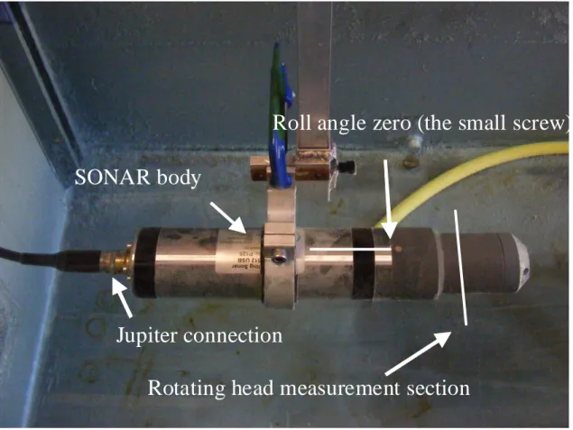
The profiler consisted in an emitter and an acoustic receiver which rotates inside the probe case, which has been made by means of an alloy cylinder of about 70 mm of diameter and about 445 mm of length. The sonar profiler (Figure 4) is provided with a rotating head that measure the acoustic backscatter along 400 beams of 0.9° each and for 250 control volume, or bin, from the centre of the probe to the maximal measured distance or range Rmax, with a frequency of 1 Hz (i.e., a section each second).

Rotating head measurement section

SONAR body

Jupiter connection

Roll angle zero (the small screw)

Figure 4 SONAR Marine Electronics model 1512.

The plane of rotation is located at around 4.5 cm from the edge of the PVC boot. The working frequency of the profiler is of 2 MHz. The probe can detect the acoustic backscatter (ABS) with maximum distances (subscript “max”) ranging between 0.125 m < Rmax < 6 m, where R is the generic position of the control volume or bin from the SONAR center. The probe is able to detect both pitch and roll angle (right bottom of the frame), with a precision of ±0.1°. Figure 5a-b show the ABS output recorded with the software “pipe profiler” in laboratory conditions and in situ conditions respectively. The black centre is automatically blanked by the software, as the zone of 20 cm of diameter is perturbed by the transducer noise. The image shows the bottom and the side walls of the channel. Generally, when the signal hit perpendicularly a surface, a large part of the signal is reflected by the walls (the red spot in the image). Vice versa, the larger is the reflection angle toward the normal direction, the smaller will be the signal intensity (see the bottom reflection in the laboratory channel figure). Further, the free surface acts as a mirror, as shown in the figure in the upper part of the image. The sonar also detects the air bubbles present in the flow which are represented as the clear spot inside the channel. As it is possible to observe from the in situ conditions, sediment deposits generally shows a different ABS compared to the concrete sidewalls, owing to the different nature of the soft deposits.

(a) SONAR output, laboratory conditions, Rmax=500 mm, the + represent the sonar center

Channel bottom

sidewalls

Free surface

Air bubbles echoes

Secondary echoes

R

Single beam

of 0.9°

(a) SONAR output, insitu conditions, Rmax =1000 mm Figure 5 pipe profiler SONAR output for PL= 4 us

The main parameters that can be regulated from the system control software are (Figure 6): • The “range” or maximum detectable distance (0.125 < Rmax < 6 m); the probe hence

presents a geometrical resolution of 1/250 of the maximum range, since each radial beam is divided in 250 control volume between 0<R<Rmax.

• The “pulse length” (4 µs <PL<20 µs), which represent the duration of the pulse

generated by the sonar; the vertical resolution δv is connected to PL by δv=cPL /2.

Free surface

Concrete walls (strong echoes)

Soft sediment

deposits

Side bank (+45 cm

from the invert

Figure 6 pipe profiler system control panel.

The output generated by the software is given in counts using an 8-bit scale. The SONAR is equipped with a 70 dB logarithmic receiver, in which the output voltage (the voltage post-processed by the probe and which is latter converted in counts) produced by the probe is proportional to the logarithm of the input voltage (the row signal recorded by the piezoelectric transducer of the SONAR). The software automatically adjusts the gain to the largest detected backscatter. However, the row image also gives the gain used for the automatic adjustment (see appendix for more details).

The software also allows the regulation of the maximal intensity and the threshold, which, however, doesn’t modify the accuracy of the measure. The temperature needs to be manually adjusted, as the probe has not been equipped with a thermometer.

A profile of the bottom can be obtained by the recorded image using three different algorithms via software. The software elaborates separately each beam or sector of 0.9°:

• “Max”, the profile is obtained from the points were the maximum ABS is detected; • “3/4”, the profile is obtained from the point were ¾ of the maximum ABS is detected; • “Area1”, the profile is obtained from the point were the largest energy is detected Figure 7 shows an example of the profile individuated by the SONAR outputs using the algorithms proposed in the pipe profiler software. The white lines in the figures show the profile individuated by the algorithms. In general, “max” shows a profiler which is more extended compared to the other two. However, slight differences occurs between them, generally less than 1 cm, whilst the profile individuated over the bottom sediment is quite scattered and shows even slighter differences amongst the three proposed algorithm.

(a) “max” algorithm insitu conditions, Rmax =1000 mm

(b) “3/4” algorithm insitu conditions, Rmax =1000 mm

(c) “AREA1” algorithm insitu conditions, Rmax =1000 mm

Figure 7 detection algorithms proposed in the Marine Electronics Pipe Profiler software Further details on the working operation are included in the appendix

4.2Sontek 10 Mhz side looking ADV

The ADV is an acoustic device which measures the three components of the instantaneous velocity u, v and w (longitudinal, transverse and vertical components respectively) according to the axis orientation shown in Figure 8. The coherent pulse ADV works with a maximum frequency of 25 Hz, allowing for the characterisation of the flow turbulence. The ADV has an operative frequency of f0=10 Mhz, owing to the shorter distance of the control volume compared to that measured by the SONAR. The ADV has one emitter at the centre of the probe and three receivers (Beam “0”, Beam “1” and Beam “2”). The receivers are focused at about 10 cm from the emitter in order to reduce the flow disturbance.

The ADV velocity measurement is based on the frequency shift of the backscattered signal:

Vi=c∆f/f0 (15)

where Vi is the velocity measured along the half bisector beam

Hence, the ADV measure the average velocity of the particles inside the control volume (about 1 cm3 and function of the geometry and the directivity of the emitter/receiver). Several parameters can be regulated when measuring the data, amongst which the most important are:

• Sample frequency fs: ranging from 1 Hz < fs <25 Hz; corresponding to the frequency used to record the instantaneous velocity;

• Velocity range Vmax: 0.03 m/s < Vmax < 250 m/s; corresponding to the Nyquist velocity, or the maximum instantaneous velocity which can be measured without aliasing.

According to the principle of pulse coherent Doppler velocity measurement, there are no limits for the lowest velocity which can be measured with the probe. However, according to the manufacturer, the precision of the measurement is about 1% of Vmax.

The half-bisector velocity from each beam is then rotated according to geometrical transformations, in order to obtain the velocity in the Cartesian system. The measure of each velocity along the half bisector of the angle beam/transmitter might be affected by an error in the estimation of the velocity, which further reduce the accuracy of the final velocity measurement in Cartesian coordinates. As example, the presence of particles larger than the control volume or high turbulence near the walls (which however is the quantity to measure) might produce a spike or peak in the velocity time-series. Hence data need to be post-processed, in order to eliminate the spike. Several criteria to assess the quality of ADV measure have been proposed. In particular two main parameters measured by the probe are of main importance:

• Signal to noise ratio (SNR): this parameter gives the ratio in dB scale of the ABS strength to the floor noise (either acoustical or electrical); generally the quality requirements need this value to be larger than 15 dB; this parameters also reflects the quantity of scatters present in the water, the larger the nb is the larger will be the SNR,

• Correlation: this parameters assess the correlation between the transmitted pulse and the received pulse; generally if the signal received comes from the scatters present in the control volume the correlation is high while in case of large turbulence the sudden changes of the particle may reduce the correlation; a good signal has a correlation larger than 70%.

Hence a first screening might be based on the analysis of those parameters. A first attempt has been done by (Wahl, 2003) based on the consideration that the acceleration of a particle cannot be larger than the gravity acceleration, otherwise the particle would escape from the flow. A second attempt has been proposed by (Goring and Nikora, 2002) and (Wahl, 2003) introduced a different algorithm to remove the spike and filter bad samples from the signal. This algorithm called “phase space threshold”, considered not only the variance of the velocity fluctuation but also the variance of the first and second derivates. According to the

for each derivate. The axis of the space can be multiplied by a level of significance, in order to improve or reduce the number of data removed. Hence all the samples outside from the space are removed. In order to evaluate other properties connected to the turbulence and the energy dissipation (such as auto and cross-correlation spectra), the filtered signal needs to be continuous, i.e., the holes left by the application of any filtering procedure needs to be fitted. In this work we adopted the technique suggested by (Wahl, 2003), in which a cubic regression is obtained for the first 7 sample after the filtered samples and the last 7 samples before the filtered one. It is worth observing that the filtering procedure is used for the three components of the velocity. Hence, if one of the component has shown a “bad” sample, the samples at the same index in the other two components of the velocity are automatically removed, owing to the fact that if one of the components contained a bad sample, the error of the measure might have propagates also to the other two components.

4.3In-situ setup

In order to achieve contemporary measurement of both sediments morphology and velocity fields, the two probes have been used in the mean time fastened together (Figure 8). The ADV has been fastened below the SONAR, in order to quickly locate its position, based on the sonar results and therefore to locate the control volume position in time effective fashion. Indeed, this specific application allows at reducing the measurements time and to improve the precision, as no need in device change is required, as well as it improves the operator’s safety, as the number of operation to carry out inside the sewer is optimised. Moreover, the measurement condition are better defined, as for each vertical, the measurements are carried out within few minutes between the first and the last survey. It is worth observing that the ADV has been fastened looking downstream, although the original configuration considered by the manufacturers is a lateral configuration. This means that velocity components need to be reoriented toward the 3 principal axes. The sketch shows the standard configuration used by the manufacturer. It is important observing that the data analysis has been carried out to ascertain whether there is any influence on the average velocity and turbulence characteristics linked to the probe orientation, although (Strom and Papanicolaou, 2007) observed that no theoretical criterion required the flow to be 2D, i.e., with zero mean transverse component.

xADV

y

ADV

z

_{AD V}

y

SONAR

x

SONAR

z

SONAR

Figure 8 ADV and SONAR fastening (same as in-situ conditions)

In the figure xADV, yADV, and zADV are coordinate referred to the sonar centre, over which the velocity component are referred, namely, u, v, and w, while xSONAR, ySONAR, and zSONAR are the system of coordinate relative to the sonar centre of rotation, which is at about 4.7mm from the probe head. The particular configuration assumed in the present test was chosen in order to:

1) allowing measurement of near interface velocity reducing the bottom interaction; 2) determining the position of the ADV control volume based on the SONAR position

toward the bottom detected by the sonar;

3) facilitating the transport and the installation of the two probes.

However, the two probes can be separated to accomplish specific tasks as further shown in the note. Velocity measurements have been carried out installing the probe in the flow orienting

xSONAR axis (and than the zADV axis) toward the x axis of the flow, and hence in the flow direction, as defined later in the text. Hence the offset between the SONAR centre and the centre of ADV control volume was fixed at 186 mm. In this configuration, the SONAR head is oriented toward the flow direction in order to reduce the disturbance effect on the flow velocity measured with the ADV.

Figure 9 Reference system definition ySONAR zSONAR xADV yADV y, v z, w x, u (flow direction) In situ reference system orientation zADV yADV xSONAR zSONAR 186 mm y, v z, w x, u (flow direction) In situ reference system orientation 186 mm Beam “0” Beam “1” Beam “2” SONAR ADV SONAR α (roll angle) β (tilt angle)

5 EXPERIMENTAL SITES, EXPERIMENTAL SETUP AND MEASUREMENTS PROCEDURE.

5.1Experimental sites

Two experimental sites have been selected, namely the “Duchesse Anne” combined sewer (DA) and the “Allée de l’Erdre” combined sewer (AE), based on the different characteristic of the flow and of both bottom and suspended sediments.

In the working section, the DA site is characterised by a slope of S=0.3‰ (Figure 10a), a catchments area of 4.11 km2, connected into a network of 21 km of length, wile the AE site has a slope of S=1.2 ‰ (Figure 10b), a catchments area of 1.41 km2 ha and a network length of about 60 km.

0

50

100

Mètres

Allée des Généraux Pa

tton et Wood Po nt d e la _R oto nd_e Allée Comm a nda nt Ch a rcot Cours John Kenne dy R ue H en ri I_V 13.70 13.70 13.70 13.70 13.70 13.70 13.70 13.70 13.70 14.05 14.05 14.05 14.05 14.05 14.05 14.05 14.05 14.05 3.6 5 3.6 5 3.6 5 3.65 3.65 3.65 3 .65 3 .65 3 .65 3 .58 3 .58 3 .58 3.5 8 3.5 8 3.58 3.58 3.58 3.5 8 2.53 2.53 2.53 2.53 2.53 2.53 2.53 2.53 2.53 3.59 3.59 3.59 3.59 3.59 3 .59 3 .59 3 .59 3.59 2.54 2.54 2.54 2.54 2.54 2.54 2.54 2.54 2.54 3 .79 3 .79 3 .79 3.7 9 3.7 9 3.79 3.79 3.79 3.7 9 5.22 5.22 5.22 5.22 5.22 5 .22 5 .22 5 .22 5.22 8.32 8.32 8.32 8.32 8.32 8.32 8.32 8.32 8.32 8.08 8.08 8.08 8.0 8 8.0 8 8.08 8.08 8.08 8.0 8 8.0 3 8.0 3 8.0 3 8.03 8.03 8.03 8.03 8.03 8.03 7.50 7.50 7.50 7.5 0 7.5 0 7.50 7.50 7.50 7.5 0 6.02 6.02 6.02 6.02 6.02 6 .02 6 .02 6 .02 6.02

(a) Duchesse Anne (DA) expertement site Flow direction