HAL Id: hal-00546280
https://hal.archives-ouvertes.fr/hal-00546280
Preprint submitted on 14 Dec 2010
HAL is a multi-disciplinary open access archive for the deposit and dissemination of sci-entific research documents, whether they are pub-lished or not. The documents may come from teaching and research institutions in France or abroad, or from public or private research centers.
L’archive ouverte pluridisciplinaire HAL, est destinée au dépôt et à la diffusion de documents scientifiques de niveau recherche, publiés ou non, émanant des établissements d’enseignement et de recherche français ou étrangers, des laboratoires publics ou privés.
Do private and public transfers received affect life
satisfaction? Evidence from Romania
Andreea Mitrut, François-Charles Wolff
To cite this version:
Andreea Mitrut, François-Charles Wolff. Do private and public transfers received affect life satisfac-tion? Evidence from Romania. 2010. �hal-00546280�
EA 4272
Do private and public transfers
received affect life satisfaction?
Evidence from Romania
Andreea Mitrut (*)
François-Charles Wolff (**)
2010/28
(*) Uppsala University and University of Gothenburg
(**) LEMNA - Université de Nantes
Laboratoire d’Economie et de Management Nantes-Atlantique Université de Nantes
Chemin de la Censive du Tertre – BP 52231 44322 Nantes cedex 3 – France www.univ-nantes.fr/iemn-iae/recherche Tél. +33 (0)2 40 14 17 17 – Fax +33 (0)2 40 14 17 49
D
o
cu
m
en
t
d
e
T
ra
va
il
W
o
rk
in
g
P
ap
er
Do private and public transfers received affect life satisfaction?
Evidence from Romania
#Andreea Mitrut
†and François-Charles Wolff
‡October 2010
Abstract
This paper uses Romanian survey data to investigate the determinants of individual life and financial satisfaction, with an emphasis on the role of public and private transfers received. A possible concern is that these transfers are unlikely to be exogenous to satisfaction. We use recursive simultaneous equations models to account both for this potential problem and for the fact that public transfers are themselves endogenous in the private transfer equation. We find that public transfers received have a positive influence on both life and financial satisfaction, while private transfers do not matter. People receive private transfers irrespective of their economic and demographic characteristics in Romania, which could be explained by some social norm motives.
Keywords: Happiness; financial satisfaction; private transfers; public transfers; Romania JEL classification: D12, D64, I31
#
We wish to thank Marcel Fafchamps, Peter Martisson, Katarina Nordblom, Henry Ohlsson for their very helpful comments and suggestions on a previous draft. Any remaining errors are our own.
†
Corresponding author. Department of Economics and UCLS, Uppsala University; Department of Economics, University of Gothenburg. Corresponding address: Box 513, SE-75120, Uppsala, Sweden. E-mail: [email protected]
‡
LEMNA, Université de Nantes, France; CNAV and INED, Paris, France.
1. Introduction
As expressed by Adam Smith (1776) and as introductory textbooks in economics teach us, “it is not from the benevolence of the butcher, the brewer, or the baker that we
expect our dinner, but from their regard to their own interest.” The homo economicus is
expected to behave as a rational and self-interested actor who desires wealth, meaning that more income should be associated with a higher level of life satisfaction in general, and of financial satisfaction in particular. In this paper, we focus on the specific effect of different income components on self-reported measures of well-being and study whether public and private transfers influence individual life and financial satisfaction.
Romania offers an interesting scenario in this context. The political crisis during Ceausescu, followed by the dramatic collapse of the economy during the first years of transition, made Romania face a severe increase in poverty.1 Public transfers were for many years chronically under-funded during Communism, and the first years of transition found them in a rapid process of disintegration. Also, while formal transfers are very limited, several authors have pointed to the importance of private transfers for the Romanian people (Mitrut and Nordblom, 2010; Amelina et al., 2004).
During the last two decades, economists have devoted a lot of attention to the determinants of subjective well-being (see Van Praag and Ferrer-i-Carbonell, 2008; Dolan et al., 2008). By focusing on the impact of public and private transfers on life and financial satisfaction, our contribution is closely linked to two lines of research.
The first one is about the determinants of life satisfaction.2 While psychologists have long been interested in understanding human life satisfaction (Diener et al., 1999), the economists’ interest in this topic started with the work of Easterlin (1974, 1995).3 Looking at the effect of income on happiness, he stated the “paradox” of the increased real growth in Western countries during the last fifty years, without any corresponding increase in the reported levels of happiness. Some studies show that absolute income matters (Oswald, 1997), while Blanchflower and Oswald (2004) find support for the fact that both relative and absolute income matter. At the same time, there is a growing literature focusing on some other aspects closely linked to self-reported well-being, like the effect of unemployment, marriage, children, and health status on overall life satisfaction. Some other studies have focused on the
1
On average, Romania experienced a negative growth rate from 1990 to 2002, as opposed to other transition countries within the region (World Bank, 2003).
2
In this paper, we use the terms happiness, life satisfaction, and individual (self-reported) well-being interchangeably. Several papers have shown that these measures are highly correlated.
3
Actually, income satisfaction evaluation based on subjective income-satisfaction questions was pioneered by van Praag (1971) and the so-called Leyden School.
role of democratic institutions and social norms on individual well-being (Frey and Stutzer, 2002, Stutzer and Lalive, 2004).
The second strand of research closely linked to the present study is the literature on private transfers among households (see Laferrère and Wolff, 2006). In the earliest papers on this topic, inter-household transfers were assumed to be altruistically motivated, implying a crowding-out effect of the private contributions by government transfers (Barro, 1974; Becker, 1974). Some authors have instead considered that transfers could be explained by self-interest concerns. Cox (1987, 1990) suggests that financial transfers to children are made in exchange for services received from them or have to be reimbursed later. Private transfers may also allow households to share risk within networks of family and friends through mutual insurance (Foster and Rosenzweig, 2001; Fafchamps and Lund, 2003).
Theoretically, there are many ways in which public and private transfers may affect life satisfaction. The obvious and presumably most important channel is a pure income effect. Since receiving transfers increases household resources, this should in turn increase both happiness and financial satisfaction. However, several other explanations may come to mind. For instance, the different income sources may reflect different degrees of permanent versus transitory income, which would be expected to affect life satisfaction differently.4 Also, receipt of private transfers could pick up aspects of life satisfaction that come directly from having friends or people to socialize with, while public transfer income may be associated with a stigma. At the same time, people may feel less satisfaction from public transfers because they feel they are entitled to them because they paid into the system.
In this paper, we study whether public and private transfers have an influence on both subjective well-being and financial satisfaction, but do not investigate the channels that lead to public and private transfers having a potentially different effect than other income. As private transfers are very common in Romania, one would expect them to have an influence on satisfaction. Curiously, the link between private inter-household transfers and life satisfaction has not been studied before.5 Our contribution is thus twofold. First, as Andrén and Martinsson (2006), we bring evidence on the determinants of happiness in Romania, but
4
Public transfer income may represent permanent income (for instance a pension received until death), which could increase happiness, whereas some component of non-transfer or private transfer income may be transitory, with an unclear effect on happiness.
5
Meier and Stutzer (2008) analyze how volunteer work influences happiness in Germany. Also, Bruhin and Winkelmann (2009) and Wolff (2006) use questions on the subjective well-being of parents and children to study the existence of altruism between these two generations, but they do not take transfers (either private or public) into consideration in their empirical analyses.
with a focus on the role of public and private transfers received. Secondly, we investigate the interplay between these two types of transfers and the possibility of a crowding-out effect.6
We rely on an unusually rich Romanian household survey to study the determinants of life and financial satisfaction. With respect to the main determinants of happiness such as income and working status, our results are in line with other findings in the literature. When disentangling the impact of the different income components, we find that both non-transfer income and public transfers have a positive and significant impact on life and financial satisfaction, while income from private transfers does not seem to matter. Our results hold when taking into account the endogeneity of both private and public transfers in the life and financial satisfaction regressions and of public transfers in the private transfer regression. Furthermore, people receive private transfers irrespective of their economic and demographic characteristics and respondents who benefit from more public transfers receive less private transfers, but the crowding out effect remains incomplete.
The rest of the paper is organized as follows. Section 2 briefly describes the Romanian context. We present the data in Section 3, while the main determinants of life and financial satisfaction in Romania are investigated in Section 4. In Section 5 we account for the potential endogeneity of private and public transfers received on satisfaction. Finally, Section 6 concludes the paper.
2. The Romanian context
From a policy of full employment during Communism, the huge restructuring process after 1991 pushed many families of workers into long-term unemployment or early retirement. From 1990 to 1993, registered unemployment rose from 0% to 10.4%, while in 2002 the number of unemployed individuals reached almost 1 million (in a country of 22 million people), accounting for almost 12% of the labor force. The first years of transition found the public transfers in a rapid process of disintegration.7 In 2001, Romania spent only 13.1% of its GDP on social protection, which was less than half of most EU countries. However, roughly 87% of Romanians receive at least one social protection transfer directly or indirectly, as household members. Also, in 2001, almost three of every ten Romanians were poor, and one out of ten was extremely poor (World Bank, 2003).
6
There are few empirical studies on the relevance of a crowding-out effect between private and public transfers. Cox and Jakubson (1995), Maitra and Ray (2003), and Jensen (2004) are interesting exceptions.
7
In 2001, the average monthly pension for the retirees outside the agricultural sector was about 1.4 million lei (roughly 40 USD). The pensioners from the former agricultural cooperatives (i.e., CAP pension) had about 271,650 lei (roughly 9 USD).
Life and financial satisfaction in Romania are thus expected to be strongly affected by the adverse economic conditions. In particular, Frey and Stutzer (2002) show that Romanians were on average less satisfied with their lives when compared to Western European countries or to the U.S. Also, Andrén and Martinsson (2006) note that one important facet of happiness in Romania is financial satisfaction. In this context, private monetary and in-kind transfers may provide an alternative to poverty and to the public social security system. In developing countries, family transfers are of vital importance for poor households for whom the marginal effect on daily expenditures is large (Adams, 2006; Maitra and Ray, 2003). Also in Bulgaria, family transfers reduce the poverty level of their recipients (Dimova and Wolff, 2008).
While formal transfers are very limited, private transfers in Romania are sizeable and very common. Amelina et al. (2004) find that gross private transfers received account for about 9 percent of the recipient household, while gross transfers given constitute more than 12 percent. Gift transfers are documented as a particularly important part of inter-household transactions, with about 90 percent of the inter-households being involved in gift transfers. Gross gifts received account for almost 12 percent of the recipients’ pre-transfer income, while gift giving (in absolute terms) is almost five times higher than transfers through the Minimum Income Guarantee national assistance program. The importance of inter-household transfers in Romania is also documented through sociological and anthropological studies (Kligman, 1988). In addition, social norms are important, providing support for widespread networks of friends, kinships, and neighbors (Marginean et al., 2004).
3. Data and descriptive statistics
We use an unusually rich household dataset collected by the World Bank for the year 2003 entitled the Romanian Transfers and Social Capital Survey (TSCS hereafter). The TSCS is a nationally representative dataset covering 2,641 households from both urban and rural areas. The methodology and a description of the data are reported by Amelina et al. (2004). The survey includes the standard demographic and socio-economic variables, including income. A key feature of the TSCS survey is that it contains very detailed questions about inter-households transfers, both financial and in-kind.
For each household head, we know whether he/she has received money from another person or household during 2002. In addition to these financial inflows, we also consider the following in-kind transfers, as they are common in Romania: receipt of food products and meals, receipt of clothes and footwear, receipt of objects or apparatus like
telephone car, tools or electronics, and receipt of animals. In both cases, these transfers could be either gifts (transfers for free), loans or exchanges of similar services, or part of an exchange when households received something different than what they have given. We sum up the values of these different transactions to get a total amount of private transfers received by the household. In the same way, we compute a total amount of private transfers given.
When investigating the determinants of life satisfaction, we rely on the following self-reported information: “All things considered, how satisfied are you with your
life as a whole these days?”. The different answers range from 1 (completely dissatisfied) to
10 (completely satisfied). Additionally, each respondent is asked about his/her household financial satisfaction: “How satisfied are you with the financial situation of your household?”. Again, the answers range from 1 (completely dissatisfied) to 10 (completely satisfied).
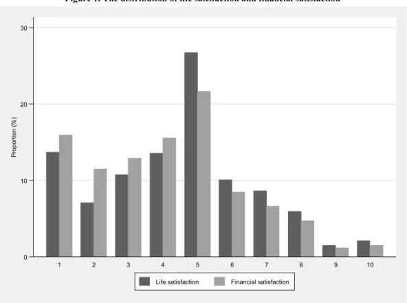
When turning to the data, we exclude from the sample all observations with non-responses for some of the questions. This reduces the size of our sample to 2,293 observations. In Figure 1, we present the distribution of the ordered measures associated with life and financial satisfaction. More than 71% of the sample report an outcome of 5 or less in response to the life satisfaction question, while the percentage is even higher (almost 78%) for financial situation. In both cases, the proportion of very satisfied respondents (8 or more) is very low (about 3%).
Insert Figure 1 here
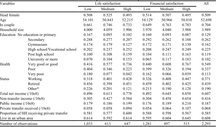
Table 1 presents the main explanatory variables used in the empirical part. Given the peak observed at the median both for life and financial satisfaction (Figure 1), we choose to aggregate the answers into three main categories: low satisfaction (values of 4 or less), medium satisfaction (5), and high satisfaction (6 or higher). Results are very similar for both happiness and financial satisfaction. Respondents living in couple are less likely to report low satisfaction. More educated individuals indicate higher life and financial satisfaction, which is also the case for those who work. Conversely, respondents with very poor or poor health report lower levels of satisfaction.
Insert Table 1 here
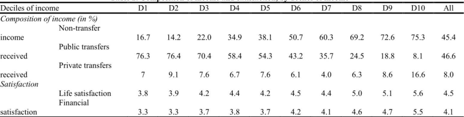
Table 2 shows the share of the three income components (respectively non-transfer income, public and private non-transfers received) by household income deciles.8 Not surprisingly, the share of public transfers received is decreasing across income distribution, while the share of private transfers received remains relatively stable across the whole
8
distribution (with a pick on the highest deciles). Both life and financial satisfaction are slightly increasing with the non-transfer income.
Insert Table 2 here
4. The determinants of life satisfaction
Let us now investigate the determinants of life satisfaction. We define by *
S
Y a latent, unobserved variable corresponding to satisfaction, either life satisfaction ( L ) or financial satisfaction ( F ). This indicator is expected to depend linearly on a set of exogenous characteristics XS (withS L,F ) such that:
S S S
S X
Y* ' (1)
By definition, we only observe the ordered indicator YS in the survey. We have YS 1 when
1 * S S Y , YS 2 when 2 * 1 S S S Y , …, and YS 10 when 9 * S S Y , where 9 1,..., S
S are a set of threshold parameters to estimate. Under the normality assumption of
the residual S, the corresponding model is a standard ordered Probit specification.9
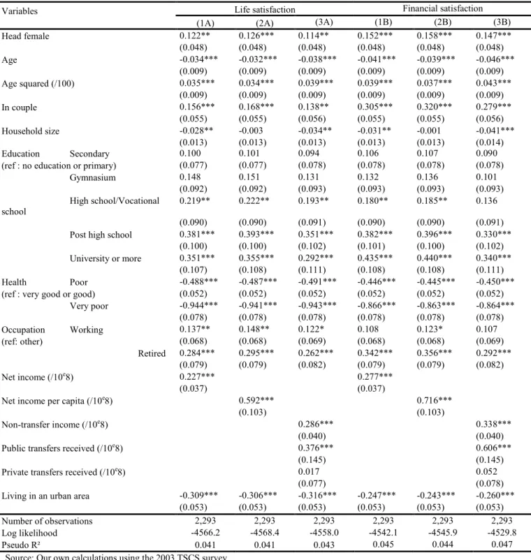
The different covariates introduced in the regressions are the standard used in this type of analyses. In particular, we account for gender, age (with a quadratic profile), living in couple, and household size, and include dummy variables for educational levels and health, activity status, net income, living in an urban area and regional dummies. The definition of net income is the sum of private income, public transfers received, and private (inter-household) transfers received minus private transfers given. For the sake of robustness, we use two measures of income: one at the household and one at the individual level.10 Estimates of the ordered Probit model are presented in Table 3, respectively columns (1A)-(3A) for life satisfaction and columns (1B)-(3B) for financial satisfaction.
Insert Table 3 here
Our main results are in line with other findings in the literature. On average, women seem happier than men, and so do individuals living in couple.11 We notice a
U-9
We have also estimated bivariate ordered Probit models to account for the potential correlation between the residuals of the life satisfaction and financial satisfaction equations and reach very similar conclusions. These additional results are available upon request.
10
As adult equivalence scales, we use the Romanian Equivalence Scale as defined by the World Bank. The Romanian Equivalence Scale assigns the following weights to the consumption of each family member: 1.0 for the first adult person, 0.8 for each additional adult person aged 15-61, 0.8 for each additional adult person aged 62 or older, 0.6 for each child aged 7-14, and 0.4 for each child aged 0-6.
11
We do not know respondent marital status (i.e., divorced, widowed, or separated), since we only observe the relation to the household head. We should be cautious about the possible reverse causality when inferring
shaped profile for age, suggesting that the least satisfied with their lives are the middle-aged cohorts. It could be that these cohorts experience a high pressure to manage both their professional and personal lives (Alesina et al., 2004). On the other hand, these are the cohorts that, after the fall of Communism, were highly exposed to the transition process. They initially formed high hopes, immediately after the Revolution – hopes that collapsed shortly after. As expected, we find a strong positive effect of education, which is likely to pick up a kind of permanent income effect, and a negative impact of poor and very poor health conditions. Living in an urban area also has a negative influence on overall life satisfaction.
Not surprisingly, both working and retired respondents have a higher life satisfaction compared to the reference group that includes housewives, persons in incapacity of work, students and registered and unregistered unemployed.12 We find a positive effect of income, meaning that money does increase life satisfaction. Similar conclusions have been reached by Andrén and Martinsson (2006) for Romania and by Alesina et al. (2004) for some European countries and for the U.S. Note that this effect is “net” of the role of family size. In Column (2A) of Table 3, we account for the level of income per capita and still get a positive coefficient. In the sequel, we only control for household income, as this covariate has been shown by Ravallion and Loskin (2001) to be a better predictor of individual life satisfaction than individual income.
We now study whether the different income components have a specific impact on life satisfaction. A very preliminary approach, based on the ordered specification presented before, is simply to introduce the three components of total income received into the life satisfaction regression. Note here that we choose to exclude amount of private transfers given, as it may be strongly related to the amount of transfers received. The key issue is to know whether life satisfaction depends on the different sources of resources at the household level. The corresponding estimates are shown in Column (3A) of Table 3. In what follows, we only focus on the income components as all our previous results remain valid.
Recalling that the bulk of household resources is non-transfer income, we find a positive and significant coefficient for this covariate. As suggested by our descriptive statistics, richer respondents seem, on average, happier. The estimate associated with income from public transfers is also positive and statistically significant. The public transfer
conclusions about the individuals living in couple (married or not), since it may be the case that happier individuals are more likely to marry/be in a relationship, since they may be better at building relations.
12
We include the unemployed together with the housewives, students and persons in incapacity of work since in our sample, less than 2% of the household heads were registered unemployed and about 2% were un-registered unemployed (meaning that they do not actively look for a job and do not receive any benefits).
coefficient is more important than the one for non-transfer income, but a Wald test indicates that the two coefficients are not significantly different from each other.13 An explanation for the strong role of public transfers could be that they are more secure than other sources of income. They are received regularly, thereby offering more financial security to the household. This could, in turn, translate into a higher level of satisfaction.14
While the coefficient associated with the amount of private transfers received is also positive, it is not significant at conventional levels. It is also statistically different from the non-transfer income and public transfer coefficients. So, public and private transfers have different effects on happiness. Two main explanations may come to mind. First, there is much more uncertainty about the receipt of private transfers, which are usually made on an irregular basis, and recipients may have poor economic characteristics that prevent them from self-reporting a high value for life satisfaction. Secondly, as highlighted in Table 2, the weight of this income component is much lower at the household level, making the income effect of this type of limited resource not sufficient to achieve a higher level of satisfaction.
When we consider financial satisfaction (Table 3, columns 1B-3B), our results are very similar to those on the life satisfaction discussed above. Only non-transfer income and public income have a positive and significant influence on financial satisfaction. One possible explanation is that in the life satisfaction regressions we actually pick up some income effects that affect the overall happiness. At the same time, we note that the public transfer coefficient is about twice higher than the non-transfer income coefficient, respectively 0.606 instead of 0.338 from column (3B). The difference between the two coefficients is significant at the 6 percent level according to a Wald test (with a statistic equal to 3.54). The greater security associated to public transfers could explain their higher impact on financial satisfaction.
5. Endogeneity issue
So far, our results have shed light on correlations between life or financial satisfaction and private and public transfers received by the household. However, these estimates remain difficult to interpret because of the following trade-off. On the one hand, the respondent is likely to be better-off with more public transfers, which should increase his/her life satisfaction. On the other hand, receiving public transfers like unemployment benefits or social allowances is also a signal that the respondent is in a poor situation, which is on a priori
13
We find a statistic equal to 0.26 for the Wald test, with a probability equal to 0.611.
14
This may not be true for the unemployed or other less well-off respondents if public transfers depend on other economic characteristics of the household. This sets up the endogeneity problem that we will examine next.
grounds associated with a lower value for life satisfaction. Thus, the private and public transfer components of income may be not exogenous in the life or financial satisfaction equations.
Several arguments help us understand the complex interrelationship between the different income components. First, virtually all models of family transfers predict that the receipt of private transfers depends on household non-transfer income. Under altruism, those in a poor economic situation should receive more money from donors, while the relation can be either positive or negative under exchange (Cox, 1987). Those with limited resources may have more time to care for their parents and thus should receive more money in exchange, but parents may also be ready to pay a higher price for attention and services from rich children. Secondly, under the assumption of dynastic intergenerational altruism, private transfers are crowded out by public transfers (Barro, 1974).15 Again, a different pattern may occur under exchange, with the possibility of a crowding-in effect (Cox and Jakubson, 1995).
Therefore, we need to account for potential endogeneity of private and public support in the satisfaction equations. At the same time, we also need to account for the fact that public transfers may themselves be endogenous in the private transfer equation. In what follows, we try to control for these two sources of endogeneity, but we choose to neglect the potential endogeneity of non-transfer income. Indeed, non-transfer income is considered exogenous in the private transfer equation in all empirical studies on family transfers (see Laferrère and Wolff, 2006).16 Another feature of the data is that only a fraction of households receive private and/or public transfers. For instance, the proportion of respondents not receiving private transfers amounts to 41.4%, while it is equal to 13.4% for public transfers. It thus matter to take censoring into account.
We hence choose to estimate recursive, simultaneous equations models comprising the three following equations: one Tobit equation for public transfers, one Tobit equation for private transfers with public transfers as an additional covariate, and one ordered Probit equation for life satisfaction (or financial satisfaction) with public and private transfers as additional regressors. This system defines the following recursive model:
15
A respondent who receives one additional unit of money through public support should receive one unit of money less through private help if the donor is perfectly altruistic.
16
In a very different setting, Maitra and Ray (2003) estimate Engel curves and study whether the different expenditure shares are influenced by the endogeneized income components (non-transfer income, private and public transfers).
S pr pr pu pu S S S pr pu pu pr pr pr pu pu pu pu T T X Y T X T X T ' ' ' * * * (2)
withTpu max(0,Tpu* ), Tpr max(0,Tpr*) and YS j when Sj YS* Sj 1 (with j 1,...,10 and S L,F ). The set of threshold values S1,..., S10 has to be estimated jointly with the different coefficients.
Assume first that the residuals pu, pr, and S follow a trivariate normal distribution, but are uncorrelated. Then, the simultaneous model defined by (2) is a recursive one, but endogeneity of transfers is not taken into account. The different estimates with a joint estimation will be very similar to those obtained through an estimation of the three separate equations. Next, if we relax the assumption of null correlations among the residuals, i.e.,
0 ) ,
cov( pu pr , cov( pu, S) 0 and cov( pr, S) 0, we get a recursive model where endogeneity is explicitly taken into account.
A central issue when estimating such models is identification. In a setting of a multiple equations Probit model with endogenous dummy regressors, Wilde (2000) shows that exclusion restrictions on the exogenous regressors are not necessary. This issue is rather similar in our context and a first source of identification stems from the non-linearity of the various equations. However, the model remains only weakly identified, so we have attempted to add exclusion restrictions in order to secure identification.
First, we include the proportion of retirees in the household in the public transfer equation. In Romania, a large proportion of public transfers occur through pensions, meaning that a household with more retirees will receive significantly more public transfers.17 At the same time, we will demonstrate that private transfers are influenced by neither the level of household income nor the occupational status of the head. Secondly, private transfers are expected to depend on public transfers. Thus, an additional variable is needed to identify the private transfer equation.
We choose to rely on a community social norm proxy. Community social norms are especially important in societies were most private transfers are between non-family members, which is the case in Romania (Kligman, 1988). Our measure is the average answer at the community level to a question on whether the respondent participated with money
17
According to our data, about 80% of the public transfers received are retirement benefits: state old pension, veterans’ pension, disability pension, and pensioners from the formal agricultural cooperatives.
and/or work in projects carried out in the community (like building a church) during the last five years. This measure is likely to capture some internalized social norms concerning private transfers’ behavior as shown in Portes (1998) and Mitrut and Nordblom (2010). In a community with strong internalized norms induced by important traditions and religious rituals (e.g., requiems and alms), people are expected to receive more transfers, a hypothesis which seems highly relevant in Romania (Mitrut and Nordblom, 2010).18
The above specification is estimated separately for the life satisfaction (Table 4) and financial satisfaction (Table 5) using a maximum likelihood method and numerical integration given the presence of multivariate integrals. Our main results are as follows.
First, in Column (1) of Table 4 and Table 5, we fix the different correlations to zero. We thus have a joint estimation of the three equations, but endogeneity does not matter. These estimates are analogous to a seemingly-unrelated model in the linear case, but we have two censored and one ordered dependent variables in our framework. Then, in Column (2) of Table 4 and Table 5, we relax the assumption of null correlations and the various estimates are net of endogeneity bias.
Insert Table 4 here
Let us first focus on the determinants of life satisfaction and more precisely on the effect of the income variables (see Table 4). Under the assumption of exogenous private and public transfers, the estimates in the last column of specification (1) show that life satisfaction increases significantly both with non-transfer income and public transfers (at the 1 percent level in both cases, respectively with t=7.14 and t=2.60). As expected, these results are very similar to those described in Table 3. Income from private transfers received also has a positive influence, but the coefficient is not significant (t=0.21). Our results on life satisfaction hold once the issue of endogeneity is taken into account (Column 2). Non-transfer income significantly increases happiness (with t=7.01), while the public transfers received are now significant at the 5.8 percent level (with t=1.90). These results suggest that endogeneity of income components is not important for life satisfaction.
Let us further investigate the determinants of public and private transfers.19 Concerning public transfers, the amount received increases with household size and when the
18
At the same time, the effect on well-being is less clear, with two offsetting effects. The household will have lower resources because the gift to the community (negative effect), while helping the community could enhance happiness (positive effect). We have checked and our social norm proxy has no influence in the satisfaction equation. We have also considered the individual participation in community projects (instead of a community average) and reach very similar results.
19
Concerning public transfers, the amount of allowances received increases with the number of older persons living in the household (62+), which is due to inclusion of pensions in public transfers. Transfers are lower when
respondent is married. An interesting finding is that public transfers increase in education. This is due to the fact that the bulk of the public transfers are pensions, which of course are higher with higher education. When it comes to private transfers received, a first finding is that they remain hard to explain. Covariates like gender, household size, education, and activity status are not significant. One possible explanation is that private transfers in Romania are motivated by social norms, so that they do not really depend on household characteristics. This implies that people receive some money or in-kind from other people regardless of their own demographic and economic situation. However, we do find that our proxy for internalized norms at the community level is positive and significant. As explained, this measure may only capture some aspects of the community-wide social norms.20
Additionally, we evidence a positive relationship between the amount of private transfers received (estimated through a Tobit equation) and the amount of non-transfer income, which casts doubt on the relevance of altruism. However, we do not control for the economic situation of the donor, this information being missing in the data set. Under the assumption of exogeneity, we find that public transfers have no influence on private transfers. However, once endogeneity is taken into account, we get a negative and significant coefficient for the amount of public transfers (with t=-2.50). This finding that respondents who benefit from more public transfers receive less private transfers is in line with a crowding-out effect. Nevertheless, the private transfer received is reduced by about 0.3 lei for each additional lei of public transfer received, meaning that the crowding-out is definitely incomplete.
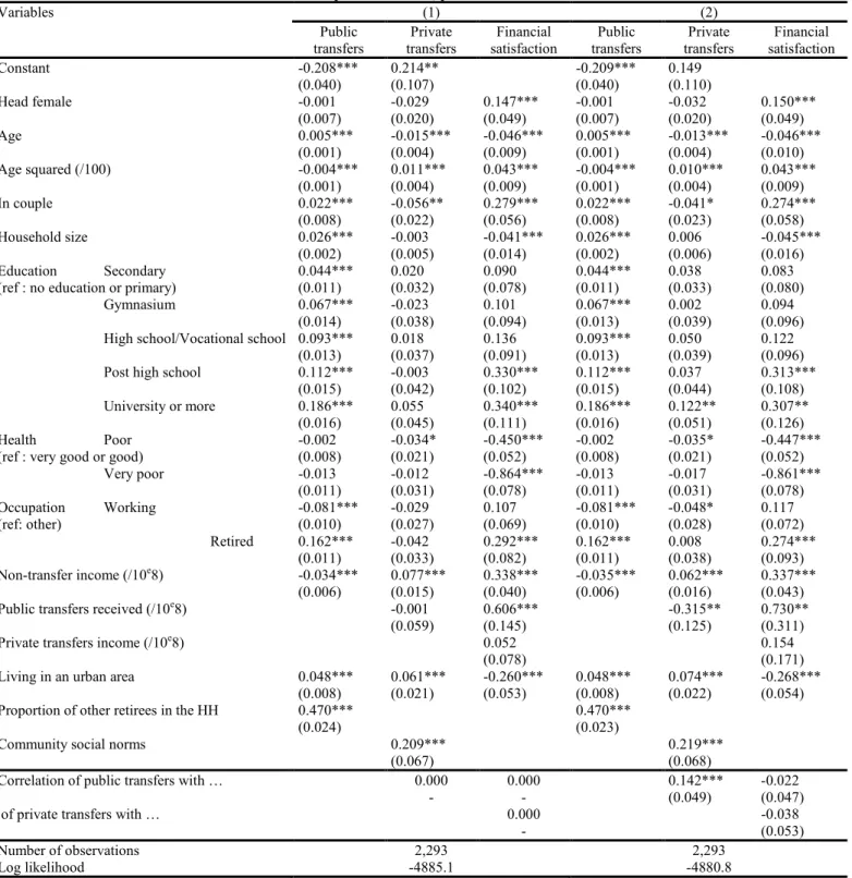
Finally, our results for financial satisfaction are very much in line with those for life satisfaction (Table 5). Under exogeneity (specification 1), the level of financial satisfaction is positively correlated with both non-transfer income and public transfers, with a much higher coefficient for the latter source of income. The recursive model which attempts to correct for potential endogeneity leads to very similar results. The amount of public transfer is significant at the 5 percent level in the financial satisfaction equation (with t=2.35) and relaxing the assumption of null correlations between the three equations of the simultaneous model does
the household head is working or unemployed, but much higher when the head is retired, and they are negatively related to the household non-transfer income.
20
Another theoretical explanation that would be consistent with this finding is a family loan model, where people first borrow money from other family members and then have to honor (and repay) their debts regardless of their economic situation (see the discussion in Laferrère and Wolff, 2006). Nevertheless, in the Romanian context, the widespread diffusion of private transfers to and from other family members, relatives, and neighbors, casts doubt on the relevance of such intertemporal exchange.
not really change the magnitude of the public transfer coefficient (0.606 under exogeneity and 0.730 under endogeneity).21
Insert Table 5 here
7. Conclusions
Using original household data from Romania, this paper has investigated the determinants of life and financial satisfaction, with a focus on the effects of private and public transfers on individual self-reported well-being measures. We find new results with respect to the existing literature on life satisfaction.
When treated as exogenous, we find that both public transfers and non-transfer income have a positive and significant impact on life satisfaction, while income from private transfers does not seem to matter. One could interpret the positive and significant impact of public transfers as evidence that these transfers are received regularly, thereby offering a stronger sentiment of security. Additionally, we find that public transfers have no effect on the private transfers received. However, a difficulty is that both private and public transfers may not be exogenous in the life satisfaction regression, while public transfers are also unlikely to be exogenous in the private transfer equation.
We estimate non-linear, recursive models to account for the potential endogeneity of the public and private transfers in the satisfaction equation. We still obtain a positive effect of non-transfer income and public transfers on both life and financial satisfaction in Romania, while private transfers do not play a significant role. Furthermore, once we control endogeneity, we do find evidence of an incomplete crowding-out effect in the public transfer equation. At the same time, in line with Mitrut and Nordblom (2010), we find that private transfers are higher in community with stronger social norms and show that very few household characteristics explain the receipt of private transfers in Romania.
From a public policy viewpoint, our results put emphasis on the extended benefits that public transfers may have on households. They are of course important sources of incomes in developing or transition economies, thereby reducing poverty and leading to better financial satisfaction. At the same time, they are much more secure than any other forms of resources. People may hence achieve higher levels of satisfaction because these transfers tend to reduce uncertainty of income, an important feature in a country where the
21
Both in Tables 4 and 5, there is only one significant coefficient of correlation. It concerns the error terms respectively associated to public transfers and private transfers. This suggests that what really matters for the estimation is the endogeneity of public transfers in the private transfer equation.
average income remains quite low. This could have in turn strong macroeconomic implications, for instance through a more permanent increase of private consumption among Romanian households.
As they stand, our results call for a deeper investigation of the mechanisms through which public and private transfers enhance life satisfaction. Having longitudinal data would be very useful to control for unobserved heterogeneity at the household level and to further study how a change in the amount of public transfers received by households influence the amount of private transfers received. Panel data could also shed light on more long term influence of the different income sources on savings or consumption. Finally, it could be of interest to study the relationship between life satisfaction and the decision to give transfers to others.
References
Adams, R. (2006). “Remittances and poverty in Ghana.” World Bank Policy Research Paper, no. 3838.
Alesina, A., Di Tella, R., MacCulloch, R. (2004). ”Inequality and happiness: are Europeans and Americans different?” Journal of Public Economics, 88: 2009-2042.
Amelina, M., Chiribuca, D., and Knack, S. (2004). “Mapped in or mapped out? The Romanian poor in inter-household and community networks.” The World Bank.
Andrén, D., Martinsson, P. (2006). “What Contributes to Life Satisfaction in Transitional Romania?” Review of Development Economics, 10(1): 59-70.
Barro, R. (1974). “Are Government Bonds Net Wealth?” Journal of Political Economy, 82(4): 1095-1117.
Becker, G. S. (1974). “A theory of social interactions.” Journal of Political Economy, 82(4):1063-1094.
Blanchflower, D., and Oswald, A. (2004). “Well-being over time in Britain and the USA.” Journal of Public Economics, 88: 1359–1386.
Bruhin, A., Winkelmann, R. (2009). “Happiness functions with preference interdependence and heterogeneity: The case of altruism within the family.” Journal of Population Economics, 22: 1063-1080.
Cox, D. (1987). “Motives for private income transfers.” Journal of Political Economy, 95(3): 508-546.
Cox, D. (1990).”Intergenerational Transfers and Liquidity Constraints.” Quarterly Journal of Economics, 105(1):187-217.
Cox, D. and Jakubson, G. (1995). “The connection between public transfers and private interfamily transfers.” Journal of Public Economics, 57(1): 129–167.
Diener, E., Suh, E., Lucas, R., Smith, H. (1999). “Subjective well-being: three decades of progress.” Psychological Bulletin, 125 (2): 276–303.
Dimova R., and Wolff F.C. (2008). “Are private transfers poverty and inequality reducing? Household level evidence from Bulgaria.” Journal of Comparative Economics, vol. 36, pp. 584-598.
Dolan, P., Peasgood, T., and White, M. (2008). “Do we really know what makes us happy? A review of the economic literature on the factors associated with subjective well-being.” Journal of Economic Psychology, 29(1): 94-122.
Easterlin, R., (1974). “Does economic growth improve the human lot? Some empirical evidence.” In: David, P., Reder, M. (Eds.), Nations and Households in Economic Growth: Essays in Honour of Moses Abramovitz. Academic Press, New York.
Easterlin, R. (1995). "Will Raising the Incomes of All Increase the Happiness of All?" Journal of Economic Behaviour and Organization, 27: 35-48.
Fafchamps, M. and Lund, S. (2003). “Risk-sharing networks in rural Philippines.” Journal of Development Economics, 71: 261-287.
Foster, A and Rosenzweig, M. (2001). "Imperfect Commitment, Altruism, and the Family: Evidence from Transfer Behavior in Low-Income Rural Areas." Review of Economics and Statistics, 83(3): 389-407.
Frey, B. S. and Stutzer, A. (2002). “Happiness and Economics: How the Economy and Institutions Affect Human Well-Being.” Princeton University Press.
Jensen, Robert. (2004). “Do private transfers ‘displace’ the benefits of public transfers? Evidence from South Africa.” Journal of Public Economics, 88: 89-112.
Kligman, G. (1988). “The wedding of the dead: Ritual, Poetics, and Popular Culture in Transylvania.” University of California Press.
Laferrère A. and Wolff F.C. (2006).“Microeconomic models of family transfers.” In S.C. Kolm, J. Mercier Ythier, Handbook on the Economics of Giving, Reciprocity and Altruism, North-Holland, Elsevier.
Maitra, P. and Ray, R. (2003). “The effect of transfers on household expenditure patterns and poverty in South Africa.” Journal of Development Economics, 71: 23-49.
Marginean, I., Precupetu, I., and Preoteasa, A. M. (2004). “Puncte de support si elemente critice in evolutia calitatii vietii in Romania.” Calitatea Vietii, 1-2.
Meier, S. and Stutzer, A. (2008). “Is Volunteering Rewarding in Itself?” Economica, 75: 39-59.
Mitrut, A. and Nordblom, K. (2010). “Social Norms and Gift Behaviour: Theory and Evidence from Romania.” Working Paper 262, Goteborg University, forthcoming European Economic Review.
Oswald, A. (1997). “Happiness and economic performance.” The Economic Journal, 107: 1815–1831.
Portes, A. (1998). “Social Capital: Its Origins and Applications in Modern Sociology.” Annual Review of Sociology, 24: 1-24.
Ravallion, M., and Lokshin, M. (2001). “Identifying welfare effects from subjective questions.” Economica, 68: 335-357.
Smith, A. (1776). “An Inquiry into the Nature and Causes of the Wealth of Nations”, ed. Edwin Cannan, London.
Stutzer, A. and Lalive, R. (2004) "The Role of Social Work Norms in Job Searching and Subjective Well-Being." Journal of the European Economic Association. 2(4): 696-719. van Praag, B. (1971). "The welfare function of income in Belgium: An empirical investigation," European Economic Review, 2 : 337-369.
van Praag, B and Ferrer-i-Carbonell, A., (2008). “Happiness Quantified: A Satisfaction Calculus Approach.” Oxford University Press.
Wilde, J. (2000). “Identification of multiple equations Probit models with endogenous dummy regressors.” Economics Letters, 69: 309-312.
Wolff, F.C. (2006). “Une mesure de l’altruisme intergénérationnel.” Economie Appliquée, 59: 5-28.
Figure 1. The distribution of life satisfaction and financial satisfaction
Source: Romanian TSCS, 2003.
Note: subjective scales for life and financial satisfaction range from 1 (completely dissatisfied) to 10 (completeley satisfied). 0 10 20 30 P ro p o rt io n ( % ) 1 2 3 4 5 6 7 8 9 10
Table 1. Descriptive statistics of the sample
Variables Life satisfaction Financial satisfaction All
Low Medium High Low Medium High
Head female 0.508 0.525 0.493 0.514 0.507 0.495 0.509
Age 54.101 50.843 52.215 54.129 50.966 50.810 52.698
In couple 0.661 0.746 0.733 0.649 0.763 0.783 0.704
Household size 4.000 4.059 3.906 3.970 4.040 3.988 3.989
Education No education or primary 0.167 0.095 0.102 0.160 0.093 0.087 0.129
Secondary 0.288 0.277 0.207 0.292 0.262 0.188 0.262
Gymnasium 0.174 0.179 0.127 0.172 0.171 0.130 0.162
High school/Vocational school 0.202 0.237 0.252 0.208 0.247 0.249 0.225 Post high school 0.100 0.108 0.159 0.104 0.111 0.163 0.119 University or more 0.070 0.104 0.153 0.065 0.117 0.183 0.102 Health Very good or good 0.416 0.577 0.736 0.440 0.608 0.767 0.549
Poor 0.404 0.346 0.223 0.399 0.326 0.194 0.337
Very poor 0.180 0.077 0.042 0.162 0.066 0.039 0.113
Status Working 0.318 0.401 0.428 0.326 0.408 0.447 0.371
Retired 0.456 0.398 0.451 0.459 0.402 0.425 0.439
Other* 0.226 0.201 0.121 0.215 0.190 0.128 0.190
Total net income (/10e8) 0.496 0.613 0.778 0.492 0.645 0.858 0.607 Non-transfer income (/10e8) 0.305 0.427 0.584 0.304 0.458 0.654 0.416
Public income (/10e8) 0.179 0.186 0.199 0.176 0.189 0.210 0.187
Private transfer received (/10e8) 0.058 0.058 0.094 0.054 0.064 0.107 0.068 Proportion of HH receiving private transfer 0.581 0.577 0.600 0.588 0.598 0.567 0.585
Live in an urban area 0.614 0.592 0.614 0.595 0.604 0.645 0.608
Number of observations 1,033 613 647 1,281 497 515 2,293
Source: Romanian TSCS survey, 2003 (our own calculations).
Table 2. Composition of income and satisfaction, by deciles of income
Deciles of income D1 D2 D3 D4 D5 D6 D7 D8 D9 D10 All
Composition of income (in %) Non-transfer income 16.7 14.2 22.0 34.9 38.1 50.7 60.3 69.2 72.6 75.3 45.4 Public transfers received 76.3 76.4 70.4 58.4 54.3 43.2 35.7 24.5 18.8 8.1 46.6 Private transfers received 7 9.1 7.6 6.7 7.6 6.1 4.0 6.3 8.6 16.6 8.0 Satisfaction Life satisfaction 3.8 3.9 4.2 4.4 4.2 4.5 4.4 5.0 5.1 5.6 4.5 Financial satisfaction 3.3 3.3 3.7 3.8 3.7 4.2 4.1 4.6 4.7 5.5 4.1
Table 3. Ordered Probit estimates of life satisfaction and financial satisfaction
Variables Life satisfaction Financial satisfaction
(1A) (2A) (3A) (1B) (2B) (3B)
Head female 0.122** 0.126*** 0.114** 0.152*** 0.158*** 0.147*** (0.048) (0.048) (0.048) (0.048) (0.048) (0.048) Age -0.034*** -0.032*** -0.038*** -0.041*** -0.039*** -0.046*** (0.009) (0.009) (0.009) (0.009) (0.009) (0.009) Age squared (/100) 0.035*** 0.034*** 0.039*** 0.039*** 0.037*** 0.043*** (0.009) (0.009) (0.009) (0.009) (0.009) (0.009) In couple 0.156*** 0.168*** 0.138** 0.305*** 0.320*** 0.279*** (0.055) (0.055) (0.056) (0.055) (0.055) (0.056) Household size -0.028** -0.003 -0.034** -0.031** -0.001 -0.041*** (0.013) (0.013) (0.013) (0.013) (0.013) (0.014) Education Secondary 0.100 0.101 0.094 0.106 0.107 0.090
(ref : no education or primary) (0.077) (0.077) (0.078) (0.078) (0.078) (0.078)
Gymnasium 0.148 0.151 0.131 0.132 0.136 0.101 (0.092) (0.092) (0.093) (0.093) (0.093) (0.093) High school/Vocational school 0.219** 0.222** 0.193** 0.180** 0.185** 0.136 (0.090) (0.090) (0.091) (0.090) (0.090) (0.091) Post high school 0.381*** 0.393*** 0.351*** 0.382*** 0.396*** 0.330***
(0.100) (0.100) (0.102) (0.101) (0.100) (0.102) University or more 0.351*** 0.355*** 0.292*** 0.435*** 0.440*** 0.340***
(0.107) (0.108) (0.111) (0.108) (0.108) (0.111) Health Poor -0.488*** -0.487*** -0.491*** -0.446*** -0.445*** -0.450*** (ref : very good or good) (0.052) (0.052) (0.052) (0.052) (0.052) (0.052)
Very poor -0.944*** -0.941*** -0.943*** -0.866*** -0.863*** -0.864*** (0.078) (0.078) (0.078) (0.078) (0.078) (0.078) Occupation Working 0.137** 0.148** 0.122* 0.108 0.123* 0.107 (ref: other) (0.068) (0.068) (0.069) (0.068) (0.068) (0.069) Retired 0.284*** 0.295*** 0.262*** 0.342*** 0.356*** 0.292*** (0.079) (0.079) (0.082) (0.079) (0.079) (0.082) Net income (/10e8) 0.227*** 0.277*** (0.037) (0.037)
Net income per capita (/10e8) 0.592*** 0.716***
(0.103) (0.103)
Non-transfer income (/10e8) 0.286*** 0.338***
(0.040) (0.040)
Public transfers received (/10e8) 0.376*** 0.606***
(0.145) (0.145)
Private transfers received (/10e8) 0.017 0.052
(0.077) (0.078)
Living in an urban area -0.309*** -0.306*** -0.316*** -0.247*** -0.243*** -0.260*** (0.053) (0.053) (0.053) (0.053) (0.053) (0.053)
Number of observations 2,293 2,293 2,293 2,293 2,293 2,293
Log likelihood -4566.2 -4568.4 -4558.0 -4542.1 -4545.9 -4529.8
Pseudo R² 0.041 0.041 0.043 0.045 0.044 0.047
Source: Our own calculations using the 2003 TSCS survey.
Note: estimates from ordered Probit models, subjective scales for life and financial satisfaction ranging from 1 (lowest) to 10 (highest). Standard errors are in parentheses, significance levels being equal to 1% (***), 5% (**) and 10% (*). Each regression also includes a set of regional dummies and a set of threshold levels. The other occupation category includes housewife, unemployed – registered and unregistered, persons in incapacity of work, students.
Table 4. Simultaneous model of public transfers, private transfers and life satisfaction Variables (1) (2) Public transfers Private transfers Life satisfaction Public transfers Private transfers Life satisfaction Constant -0.208*** 0.214** -0.208*** 0.150 (0.040) (0.107) (0.040) (0.110) Head female -0.001 -0.029 0.114** -0.001 -0.032 0.113** (0.007) (0.020) (0.048) (0.007) (0.020) (0.049) Age 0.005*** -0.015*** -0.038*** 0.005*** -0.013*** -0.040*** (0.001) (0.004) (0.009) (0.001) (0.004) (0.010) Age squared (/100) -0.004*** 0.011*** 0.039*** -0.004*** 0.010*** 0.040*** (0.001) (0.004) (0.009) (0.001) (0.004) (0.009) In couple 0.022*** -0.056** 0.138** 0.022*** -0.041* 0.124** (0.008) (0.022) (0.056) (0.008) (0.023) (0.058) Household size 0.026*** -0.003 -0.034** 0.026*** 0.006 -0.040** (0.002) (0.005) (0.014) (0.002) (0.006) (0.015) Education Secondary 0.044*** 0.020 0.094 0.044*** 0.039 0.083
(ref : no education or primary) (0.011) (0.032) (0.078) (0.011) (0.033) (0.079)
Gymnasium 0.067*** -0.023 0.131 0.067*** 0.002 0.112
(0.014) (0.038) (0.093) (0.013) (0.039) (0.095) High school/Vocational school 0.093*** 0.018 0.193** 0.093*** 0.050 0.174*
(0.013) (0.037) (0.091) (0.013) (0.039) (0.095) Post high school 0.112*** -0.003 0.351*** 0.112*** 0.037 0.326***
(0.015) (0.042) (0.102) (0.015) (0.044) (0.108) University or more 0.186*** 0.055 0.292*** 0.186*** 0.121** 0.253**
(0.016) (0.045) (0.111) (0.016) (0.051) (0.125)
Health Poor -0.002 -0.034* -0.491*** -0.002 -0.035* -0.494***
(ref : very good or good) (0.008) (0.021) (0.052) (0.008) (0.021) (0.052)
Very poor -0.013 -0.012 -0.943*** -0.013 -0.017 -0.941*** (0.011) (0.031) (0.078) (0.011) (0.031) (0.078) Occupation Working -0.081*** -0.029 0.122* -0.081*** -0.048* 0.132* (ref: other) (0.010) (0.027) (0.069) (0.010) (0.028) (0.071) Retired 0.162*** -0.042 0.262*** 0.162*** 0.008 0.229** (0.011) (0.033) (0.082) (0.011) (0.038) (0.092) Non-transfer income (/10e8) -0.034*** 0.077*** 0.286*** -0.035*** 0.062*** 0.302*** (0.006) (0.015) (0.040) (0.006) (0.016) (0.043)
Public transfers received (/10e8) -0.001 0.376*** -0.314** 0.583*
(0.059) (0.145) (0.126) (0.307)
Private transfers income (/10e8) 0.017 -0.083
(0.077) (0.172)
Living in an urban area 0.048*** 0.061*** -0.316*** 0.048*** 0.074*** -0.321*** (0.008) (0.021) (0.053) (0.008) (0.022) (0.054) Proportion of other retirees in the HH 0.470*** 0.469***
(0.024) (0.023)
Community social norms 0.209*** 0.211***
(0.067) (0.068)
Correlation of public transfers with … 0.000 0.000 0.141*** -0.035
- - (0.050) (0.046)
of private transfers with … 0.000 0.029
- (0.053)
Number of observations 2,293 2,293
Log likelihood -4913.4 -4908.9
Source: our own calculations, using the TSCS survey.
(1) is a joint model comprising one Tobit equation for public transfers, one Tobit equation for private transfers, and one ordered Probit equation for life satisfaction. (2) is a simultaneous recursive model with two Tobit equations and one ordered Probit equation, public transfers being endogenous in the private transfer equations and private and public transfers being endogenous in the life satisfaction equation. Standard errors are in parentheses, significance levels being equal to 1% (***), 5% (**), and 10% (*). Each regression also includes a set of regional dummies and the ordered Probit equation for life satisfaction includes a set of threshold levels. The other occupation category includes housewife, unemployed – registered and unregistered, persons in incapacity of work, students.
Table 5. Simultaneous model of public transfers, private transfers and financial satisfaction Variables (1) (2) Public transfers Private transfers Financial satisfaction Public transfers Private transfers Financial satisfaction Constant -0.208*** 0.214** -0.209*** 0.149 (0.040) (0.107) (0.040) (0.110) Head female -0.001 -0.029 0.147*** -0.001 -0.032 0.150*** (0.007) (0.020) (0.049) (0.007) (0.020) (0.049) Age 0.005*** -0.015*** -0.046*** 0.005*** -0.013*** -0.046*** (0.001) (0.004) (0.009) (0.001) (0.004) (0.010) Age squared (/100) -0.004*** 0.011*** 0.043*** -0.004*** 0.010*** 0.043*** (0.001) (0.004) (0.009) (0.001) (0.004) (0.009) In couple 0.022*** -0.056** 0.279*** 0.022*** -0.041* 0.274*** (0.008) (0.022) (0.056) (0.008) (0.023) (0.058) Household size 0.026*** -0.003 -0.041*** 0.026*** 0.006 -0.045*** (0.002) (0.005) (0.014) (0.002) (0.006) (0.016) Education Secondary 0.044*** 0.020 0.090 0.044*** 0.038 0.083
(ref : no education or primary) (0.011) (0.032) (0.078) (0.011) (0.033) (0.080)
Gymnasium 0.067*** -0.023 0.101 0.067*** 0.002 0.094
(0.014) (0.038) (0.094) (0.013) (0.039) (0.096) High school/Vocational school 0.093*** 0.018 0.136 0.093*** 0.050 0.122
(0.013) (0.037) (0.091) (0.013) (0.039) (0.096) Post high school 0.112*** -0.003 0.330*** 0.112*** 0.037 0.313***
(0.015) (0.042) (0.102) (0.015) (0.044) (0.108) University or more 0.186*** 0.055 0.340*** 0.186*** 0.122** 0.307**
(0.016) (0.045) (0.111) (0.016) (0.051) (0.126)
Health Poor -0.002 -0.034* -0.450*** -0.002 -0.035* -0.447***
(ref : very good or good) (0.008) (0.021) (0.052) (0.008) (0.021) (0.052)
Very poor -0.013 -0.012 -0.864*** -0.013 -0.017 -0.861*** (0.011) (0.031) (0.078) (0.011) (0.031) (0.078) Occupation Working -0.081*** -0.029 0.107 -0.081*** -0.048* 0.117 (ref: other) (0.010) (0.027) (0.069) (0.010) (0.028) (0.072) Retired 0.162*** -0.042 0.292*** 0.162*** 0.008 0.274*** (0.011) (0.033) (0.082) (0.011) (0.038) (0.093) Non-transfer income (/10e8) -0.034*** 0.077*** 0.338*** -0.035*** 0.062*** 0.337*** (0.006) (0.015) (0.040) (0.006) (0.016) (0.043)
Public transfers received (/10e8) -0.001 0.606*** -0.315** 0.730**
(0.059) (0.145) (0.125) (0.311)
Private transfers income (/10e8) 0.052 0.154
(0.078) (0.171)
Living in an urban area 0.048*** 0.061*** -0.260*** 0.048*** 0.074*** -0.268*** (0.008) (0.021) (0.053) (0.008) (0.022) (0.054) Proportion of other retirees in the HH 0.470*** 0.470***
(0.024) (0.023)
Community social norms 0.209*** 0.219***
(0.067) (0.068)
Correlation of public transfers with … 0.000 0.000 0.142*** -0.022
- - (0.049) (0.047)
of private transfers with … 0.000 -0.038
- (0.053)
Number of observations 2,293 2,293
Log likelihood -4885.1 -4880.8
Source: our own calculations, using the TSCS survey.
(1) is a joint model comprising one Tobit equation for public transfers, one Tobit equation for private transfers, and one ordered Probit equation for financial satisfaction. (2) is a simultaneous recursive model with two Tobit equations and one ordered Probit equation, public transfers being endogenous in the private transfer equations and private and public transfers being endogenous in the financial satisfaction equation. Standard errors are in parentheses, significance levels being equal to 1% (***), 5% (**), and 10% (*). Each regression also includes a set of regional dummies and the ordered Probit equation for financial satisfaction includes a set of threshold levels. The other occupation category includes housewife, unemployed – registered and unregistered, persons in incapacity of work, students.