Comparison of SAGE and classical multi-antenna algorithms for multipath mitigation in real-world environment

To cite this document:

Rougerie, Sébastien and Konovaltsev, Andriy and Cuntz,

Manuel and Carrie, Guillaume and Ries, Lionel and Vincent, François and

Pascaud, Romain Comparison of SAGE and classical multi-antenna algorithms

for multipath mitigation in real-world environment. (2010) In: 5th ESA Workshop

on Satellite Navigation Technologies and European Workshop on GNSS Signals

and Signal Processing (NAVITEC 2010), 8-10 Dec 2010, Noordwijk, The

Netherlands..

O

pen

A

rchive

T

oulouse

A

rchive

O

uverte (

OATAO

)

OATAO is an open access repository that collects the work of Toulouse researchers and

makes it freely available over the web where possible.

This is an author-deposited version published in:

http://oatao.univ-toulouse.fr/

Eprints ID: 5231

Any correspondence concerning this service should be sent to the repository

administrator:

[email protected]

Comparison of SAGE and Classical Multi-Antenna

Algorithms for Multipath Mitigation in Real-World

Environment

Sébastien ROUGERIE ONERA/CNES/ThalesAleniaSpace

Toulouse, France [email protected] Andriy KONOVALTSEV, Manuel CUNTZ

DLR, Wessling, Germany [email protected], [email protected] Guillaume CARRIE ONERA Toulouse, France [email protected] Lionel RIES CNES Toulouse, France [email protected]

François VINCENT, Romain PASCAUD ISAE

Toulouse, France

[email protected], [email protected]

Abstract: The performance of the Space Alternating Generalized

Expectation Maximisation (SAGE) algorithm for multipath mitigation is assessed in this paper. Numerical simulations have already proven the potential of SAGE in navigation context, but practical aspects of the implementation of such a technique in a GNSS receiver are the topic for further investigation. In this paper, we will present the first results of SAGE implementation in a real world environment.

Keywords; SAGE,multipath, antenna array

I. INTRODUCTION

In Global Navigation Satellite Systems (GNSS) applications, multipath (MP) errors are still one of the major error sources in conventional receivers. The additional signal replicas due to reflections introduce a bias in Delay Lock Loops (DLL), which finally leads to a positioning error. Several techniques have been developed for multipath mitigation or estimation. Conventional approaches, such as Narrow Correlator Spacing [1] or Multipath Estimating Delay-Lock-Loop (MEDLL) [2] algorithm, try to mitigate the MP on the time and frequency domains. Thus, these approaches propose limited MP rejection capability in presence of short delay multipath (< 0.1 chip) [2]. More recently, the use of antenna array algorithms has been proposed for multipath mitigation. Antenna arrays perform a spatial sampling that makes possible the discrimination of sources in the space domain (azimuth and elevation) [3]. If we assume that the space domain is independent of the time domain, we can expect to mitigate very short delay MP. Moreover, by combining the energy of the useful signals received by multiple antennas, the antenna arrays are able to

significantly improve the performance of GNSS receivers under unfavourable signal conditions.

Two solutions are investigated to mitigate multipath with an antenna array. The first one tries to filter the multipaths in the space domain only in order to "clean" the incoming signal of all the multipaths. The time-delay and Doppler estimations of the Line Of Sight (LOS) signal are done after the space filtering step. In the second approach, a set of parameters (amplitudes, times-delays, Doppler shifts, elevations and azimuths) for all the incoming sources is estimated. The main difference between the approaches is that the parameter estimation in the second approach explores the signal properties on the space, time and frequency domains instead of just filtering the sources in the space domain only. To estimate the parameters of all the sources, Space Alternating Generalized Expectation Maximisation (SAGE) algorithm [4], which is a low-complexity generalization of the Expectation Maximisation (EM) algorithm, has been considered. SAGE algorithm is usually used in communication systems like in [4], but the potential of SAGE in a navigation context has been proven in [5].

The results discussed in the literature are often obtained by numerical simulations leaving the practical aspects of the implementation of such a technique in a GNSS receiver to be the topic for further investigation. Several measurement campaigns have been done in order to test these algorithms in a real world environment. The measurements were done with the 2x2 square antenna array [6, 7] operating in GPS L1 band. The paper will presents the first results obtained by using SAGE algorithm with these real world measurement data.

This paper is organized as follows. The signal model is outlined in Section II. The description of the beamforming

approach (space filtering of the multipaths) is presented in Section III. A short introduction to maximum likelihood estimation and a description of SAGE algorithm is given in Section IV and in section V we present the main results obtained by Monte-Carlo simulations. In section VI, the details about antenna array and the real world measurement campaigns are presented. The corresponding results of post-processing are then described and discussed in section VII. Finally, some conclusions are drawn in the Section VIII at the end of the paper.

II. SIGNAL MODEL

Let's assume we receive L narrowband planar wave fronts of wavelength λ on an array of m independent and isotropic sensors. Under these assumptions, the received signal after down conversion can be modelled as a superimposition of L baseband signals and an additional complex white Gaussian

noise

( )

2 , 0 ~ ) (t N σn b

( )

( ) ) ( 1 0 t t t L l l b s y =

∑

+ − = (1) with s_l

( )

t given by

( )

( _l, _l) _l exp(2 . _l.) ( _l) l t =a

θ

ϕ

×

γ

× j

π

ν

t ×ct−

τ

s (2)

where L is the number of incoming paths (LOS signal included) and Ψl = [θl, φl, γl, υl, τl]T are respectively the elevation, azimuth, complex amplitude, Doppler shift and time delay of the l path. Note that the index l=0 corresponds to the LOS signal. Here, c denotes the pseudo-random-noise sequence that consists of a Gold code as used for the GPS C/A code signal with a code period T = 1 ms, 1023 chips per code period (i.e. a time duration Tc = 977.52 ns), and a rectangular chip shape. a represents the steering vector of a 2x2 square antenna array. The antenna spacing is λ/2 and the reference of the array is on the first element. The channel parameters are assumed constant during the observation time and the received signal

) (t

y is sampled at the rate fs. = 10 MHz. Collecting the samples of the observation interval leads to

( )

Ψ B S Y=

∑

+ − = 1 0 L l l (3)

where Y, Sl and B are 4×N complex matrix with N the number of samples andΨ=

[

Ψ₀ L Ψ_L−1

]

.

In GNSS, the power of the incoming signals is usually much lower than the receiver noise level. Thus, if we want to be able to detect the GNSS signals (LOS+MP), we first need to correlate the incoming signal with the reference local code as it's presented in Figure 1. Let the integration time of the cross-correlation between the incoming signal and the reference code

be Tint and the DLL and FLL errors be ετ and ευ, respectively. The nth output of one correlator is:

(

)

[

]

∫

− + − × − − − × = int int ) 1 ( 0 0 int , . ). .( 2 exp ) ( ) ( 1 , , nT T n l l C dt t j t c t c T n R ν τ ν τ ε ν π ε τ τ ε ε (4)

We introduce the relative delay and the relative Doppler of the lth paths with respect to the LOS signal

0 0,ν ν ν

τ τ

τrl= l− rl= l− , we can approximate the integral and

write the post correlated signal as:

(

)

) ( , , ~ ~ ) , ( ) ( int 1 0 int int nT n R nT T L l rl rl C l l l b a x + − − × × =

∑

− = ν ε τ ε γ ϕ θ τ ν (5) with

(

, ,

) (

)

exp

(

2

(

)

int

)

~ nT j r n RC ετ −τrl εν −νrl = ετ −τrl × − π εν −νrl (6)

where r(.) denotes the auto-correlation function of the PRN code,

γ

~

_l the modified complex amplitude of the lth paths and

)

(

_int

int

nT

T

b

, the noise after the correlation step.

Figure 1. Space filtering after the correlation process [3]

III. BEAMFORIMG ALGORITHMS

We remind the reader that we focus our attention on multipath mitigation only. Consequently, we need to work with the post correlated signal defined in (5). The beamformer output is given by the following expression:

(

nT_int

)

(nT_int)

x H

where w is the beamformer weight vector and x

(

nTint

),

defined in (5), is the vector of array outputs. The adaptation of the weight vector w for obtaining better signal reception with respect to some criterion is the purpose of a beamforming algorithm. A number of beamformers were proposed for the use with GNSS receivers [8].

• Conventional beamforming without constraints

• Minimum Power Distortionless Response (MPDR)

• Minimum Mean Square Error (MMSE)

For these 2 last kinds of beamformers, we need to have an estimate of the correlation matrix. This matrix is usually estimated as the sample covariance matrix using a set of the available data.. In our case, we use Nms outputs of the non-delayed correlator (prompt correlator), and the integration time is Tint=1ms.

∑

= = Nms n H ms x nT nT N 0 int int) ( ) ( 1 ˆ _{x x} R (8)

Last, an estimation of the DOAs can be required for the implementation of the beamforming algorithms. Almanac data and/or an inertial navigation system can be used to provide this information. In this paper, we use 2D Unitary ESPRIT algorithm [9] to estimate the DOAs of the different incoming signals.

IV. MAXIMUM LIKELIHOOD ESTIMATION:SAGE

The problem is to estimate the parameters

[

, , , ,

]

, =0,1,2,..., −1

= l l l rl rl T l L l γ θ ϕ τ ν

ψ of the sources. The

estimation of L is not discussed in this work. Usually, L is fixed to a value large enough to capture all the dominant impinging waves. Classical information theory methods for model selection like Akaike's and Rissanen's [10] criteria can be used to estimate L.

The likelihood function for the sampled baseband signal is

( )

(

[

Y S

( )

Ψ

]

Σ

[

Y S

( )

Ψ

]

)

Σ Ψ Y = −vec − −1vec − p _N exp H det 1 π (9) where

( )

∑

( )

− =

=

1 0 L l l

Ψ

S

Ψ

S

contains the superimposed impinging wave fronts and

Σ

denotes the covariance matrix of the noise. As we assume spatially and temporally uncorrelated elements and a centered Gaussian noise, the covariance matrix of the noise is

Σ

=

σ

_n2

I

where

σ

_n2 is assumed to be known. The Maximum Likelihood Estimation (MLE) is given by:

( )

YΨ Ψ Ψ p max arg ˆ ₌ (10)

The maximization of the likelihood function is a computationally prohibitive task since there is no analytical solution in the general case. Moreover, p

( )

YΨ is not generally a concave function of Ψ, and L have usually a high dimension. In other words, we have to solve a 4×L dimensions non linear optimization problem.

To perform the optimization process, we use the iteration process of the SAGE algorithm [4]. The basic concept of the SAGE algorithm is the hidden data space [4]. Instead of estimating the parameters of all impinging waves in parallel in one iteration step as done by the EM algorithm, the SAGE algorithm sequentially estimates the parameters of each signal. Moreover, SAGE algorithm breaks down the multi-dimensional optimization problem into several smaller problems. In [5], it can be seen that SAGE algorithm is efficient for the entire multipath configuration (especially small relative delays and close DOAs) and space-time-frequency approach shows better performance than classical time-frequency approach. Nevertheless, the computational cost increases due to the maximization together on the space, time and frequency domains. Furthermore, the memory requirements also increase since it is necessary to store in the receiver the incoming signal in order to apply SAGE estimation. For example, to process 10 ms of signal with a 2 MHz sampling rate, we need to store a matrix of m×2.104 with

m the number of antennas. In other words, SAGE algorithm is

hard to implement for real time operation and therefore only offline post processing is considered in this paper.

V. SIMULATION RESULTS

The input power of the LOS signal is set to -155 dBW, and the noise power is equal to -131.9 dBW. Thus, the pre-correlation SNR is around -23 dB. The parameters of the LOS signal are: θ0 = 60°, φ0 = 131°, υ0 = 100 Hz. In order to assess the performance of the algorithms with respect to the delay estimation of the LOS for GNSS receiver, we have analyzed the behavior of our estimators for a single reflective multipath. The reflected multipath and the LOS are considered to be in-phase which corresponds to one of the worst possible cases. The signal-to-multipath ratio (SMR) is 3 dB for all reflections, and the relative Doppler is equal to 20Hz. The parameter estimations are quantized to a resolution of 0.5 ns for the delay, 0.5 Hz for the Doppler and 0.1° for the DOA.

We remind the reader that this study is focused on algorithms for a 2x2 square antenna array. With such a small antenna array, conventional beamforming (space Fast Fourier Transform) turns out to be inefficient due to the low directivity of the array. In order to improve the resolution, adaptive beamformers have been tested. Unfortunately, the LOS and multipath signals are strongly correlated and thus, classical adaptive algorithms are not able to distinguish between the LOS and the multipaths signals. On the one hand, the MPDR solution is quite sensitive to multipath components as the beamformer mitigates all the contributions in order to minimize total output power (i.e., LOS signal can be cancelled). On the other hand, the MMSE beamformer tends to constructively combine the multipath components with the signal of interest.

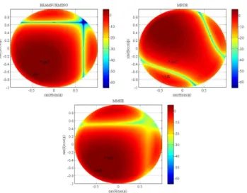
Thus, a secondary lobe in the MP direction can be created. As a consequence, the propagation delay of the LOS signal cannot be accurately obtained. In other words, MPDR and MMSE algorithms can seriously degrade the time delay estimation of the LOS in presence of MP, and should not be used in this context. In the following figure, we give some examples of space spectrum for the above discussed beamformers. For the conventional, MPDR and MMSE beamformers, the multipath has the following DOA: θ1 = 30°, φ1 = 140°.

Figure 2. Example of space spectum obtained with a CBF (top on the left),

MPDR (top on the right) and MMSE (bottom in the center) Beamformers

Another solution to reject the multipaths is to combine estimation algorithms and rejection algorithms. In this paper, we propose to use the 2D Unitary ESPRIT algorithm [9] to estimate the DOA of the incoming sources (LOS and MP). In Figure 3. we plot the Root Mean Square Error (RMSE) of the azimuth estimation of the LOS signal in the case of SAGE and ESPRIT algorithms. We plot the RMSE as a function of the relative azimuth and the relative Doppler of the MP with respect to the LOS. The relative azimuth represents how close in space is the MP and the relative Doppler, how coherent is the MP with the LOS signal. The relative delay of the MP is fixed to τr1 = 0.25 chip and the elevation to θ1 = 30°. The RMSE was calculated over 50 Monte-Carlo simulations. As we can see, in the case where the LOS and the MP are strongly correlated (very small relative Doppler), ESPRIT algorithm can result in a large error.

Consequently, if we filter spatially the MP based on the ESPRIT DOA estimation, this error can lead to a bad MP rejection. To illustrate it, we used for example an MPDR beamformer with additional null constraints in the MP direction. After the beamforming step, we used a maximum likelihood estimator (one antenna/one path SAGE algorithm) to estimate the time-delay of the LOS signal. In Figure 4. we plot the RMSE of the delay estimation after a MPDR beamforming with additional null constraints and the full SAGE algorithm (4 antennas/two paths search). Two disadvantages can be observed when using the combinations of EPSRIT and MPDR algorithms. First of all, in the case of closely spaced sources,

the MPDR beamformer seems unable to correctly reject the MP. This is mainly due to the small size of the array wich implies a low directivity and consequently, low rejection in the null direction. The second problem occurs when both sources are strongly correlated. In this condition, we already saw that ESPRIT algorithm can not provide an accurate estimation of the DOA. Consequently, the rejection, or in other words the null direction, will not be in the MP DOA. Consequently, the MP will be not completely mitigated and will continue to bias the time delay estimation of the LOS signal.

0 50 100 150 0 10 20 0 20 40 60 80 RELATIVE AZIMUTH (°) RMSE(φ_LOS) RELATIVE DOPPLER (Hz) (° ) SAGE ESPRIT

Figure 3. RMSE of the LOS azimuth estimation for the ESPRIT and SAGE

algorithms. 0 50 100 150 0 5 10 15 20 10-3 10-2 10-1 RELATIVE AZIMUTH (°) RMSE(τ_LOS) RELATIVE DOPPLER (Hz) (C H IP S ) SAGE ESPRIT/MPDR

Figure 4. RMSE of the LOS delay estimation for the ESPRIT+MPDR+ (one

antenna/one path SAGE algorithm), and the 2 paths SAGE algorithm

We can see that SAGE approach provides a real improvement in the DOA estimation. First of all, SAGE algorithm uses the frequency domain to filter a part of the Gaussian noise and then reduces its influence. In the case of close MP, SAGE has two more dimensions (Doppler and time-delay) to better discriminate the LOS signal and the MP and

thus, it provides a better estimation. Consequently, time-delay estimation is also strongly improved. To conclude, SAGE takes the advantage of the space filtering which is the possibility to reject very short delay MP [5] (an example is given in section 6), without the inconvenient which is a possible degradation of the performance for closely spaced and correlated sources.

VI. EXPERIMENTAL MEASUREMENTS

A. Antenna array description

The antenna array used for the data acquisition is a 2-by-2 uniform rectangular array with half-wavelength antenna spacing. The array is designed for operation in GPS/Galileo L1 frequency band and reception of right-hand circularly polarised (RHCP) signals. The schematic view of the antenna array is shown in the following figure.

Figure 5. Schematic view of the antenna array

For improving the polarisation purity (i.e. decreasing the axial ratio for RHCP), the patch elements are sequentially rotated by 90 degrees against each other. High polarisation purity is considered to be very helpful to minimise the effect of strong reflected multipath echoes that are expected to have left hand circular polarisation (LHCP). In [11], it can be observed that the separation between the two polarisations is better than 20 dB. More details about the characteristics of the antenna array can be found in [11].

B. Measurement set-up

With the antenna array, several sets of measurements have been done. Here, we present only the processing of two sets of measurements.

The first sets of measurements were presented in [7]. The measurements were carried out by using the set-up on the roof of a building in almost open sky conditions. Due to that, the antenna array was able to receive 9 signals of all the visible GPS satellites at the time of the signal recording (12 August 2009, 11:03 UTC). Also, we can assume that no multipaths were present during this set of measurements and thus, this scenario can be considered as a soft multipath scenario.

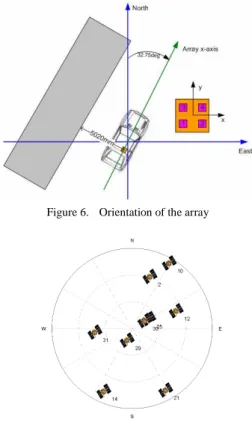
In the second set of measurements, the array was fixed on a Van situated at 5m of a metallic wall (Hangar) as we can see on the Figure 6. In this position, the array was able to receive 9 satellites (see Figure 7. ) at the time of the signal recording (2 September 2010, 14:45 UTC). The orientation of the antenna array with respect to the northeast- up geodetic coordinates is shown in Figure 6. The true DOA of each satellite, given in the antenna reference, are reported in table 1. In this condition, we

expected to see strong and static multipaths. This scenario can be considered as a hard multipath scenario.

Figure 6. Orientation of the array

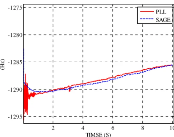
Figure 7. GPS constelation at the time of measurement

TABLE I. SATTELITE DOA

PRN 2 PRN 10 PRN 12 PRN 14 PRN 21 PRN 25 PRN 29 PRN 30 PRN 31 Elev (°) 28.20 5.46 36.62 12.78 11.27 68.29 75.86 73.07 48.21 Az (°) 19.05 29.59 68.15 -155 -208 59.59 -157 58.33 -90.6

VII. EXPERIMENTAL RESULTS

After the RF stage filter and the down conversion stage, the baseband signal can be stored at the rate of fs=2.5MHz with a 8 bits quantization. The baseband signal is then used to test the SAGE algorithm in post processing. It is also possible to store the output of the correlators at each ms of integration. With such information, it is possible to implement the algorithms presented in the section III (already implemented in the array FPGA [3]).

A. Results for the soft multipath scenario

In order to compare the performance of the different algorithms, we proceeded several tests. First of all, we were not able to know the exact position of the receiver and thus, we can not have access to the true time-delay. However, the true

DOAs of the satellites are known, and we can compare the estimated parameters with the true ones. Also, the variance of the estimation can provide an idea about the accuracy of the algorithm.

After the acquisition step and the bit transition detection, we processed the data each 20ms, and the following algorithms were used for each tracked satellite signal:

• ESPRIT: DOA estimation

• MMSE beamforming (after 1s)

• DLL: Coherent dot product discriminator, integration time of 20ms, Loop filter bandwidth of 10Hz

• PLL: atan phase discriminator, integration time of 20ms, Loop filter bandwidth of 1Hz

The beamforming algorithm and the DOA estimation algorithm were activated 3 seconds after the acquisition.

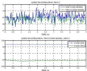
With the sampled baseband signal, we implement the SAGE algorithm to track the parameters (DOA, delay and Doppler) of the LOS signal. Here is an example of the results with the PRN 9. In Figure 8. and Figure 9. we plot the DOA estimation for the SAGE and the ESPRIT algorithms. In Figure 10. the Doppler estimation with the SAGE algorithm and PLL are presented. 0 2 4 6 8 10 12 28 30 32 34 36 38 TIME (S) (° ) ELEVATION ESTIMATION ESPRIT SAGE TRUE ELEVATION

Figure 8. Elevation estimation, PRN 9

0 2 4 6 8 10 12 -180 -178 -176 -174 -172 -170 -168 -166 TIME (S) (° ) AZIMUTH ESTIMATION ESPRIT SAGE TRUE AZIMUTH

Figure 9. Azimith estimation, PRN 9

2 4 6 8 10 -1295 -1290 -1285 -1280 -1275 TIMSE (S) (H z ) PLL SAGE

Figure 10. Doppler estimation, PRN 9

We can see that the DOA estimation is a little bit biased. That should come from some residual calibration error. However, the bias is acceptable if we compare with the directivity of the array [8]. If we now compare the standard deviation, ESPRIT algorithm seems to provide better performance in term of DOA estimation (ESPRIT: σelev=0.29°, σaz=0.29°, SAGE: σelev =0.7°, σaz=1°). But this does not lead to a better Doppler estimation. Indeed, for the Doppler estimation, we can see that SAGE and PLL algorithms have the same behaviour. Discussion of these effects will be done in the sub part C.

B. Results for hard multipaths scenario

In this section the data of each satellite have been processed for different configurations of SAGE. In the first configuration, we assume that no multipaths are present and we search only one path. This configuration is so called the one path SAGE model. In a second time, we force the SAGE algorithm to search two paths. The main idea is to track the LOS signal with one path, and have another "free path" in order to detect and track a possible multipath. This configuration is so called the two paths SAGE model.

After bit transition detection, we use 20ms to process the parameters estimation.

1) Delay estimation

In Figure 11. we give an example of relative delay estimation with the satellite number 12. In the case of the 2 paths model, we can see that the estimations of the LOS delays are very close to the one path model. We can think that no multipath was detected and the track of a second path looks useless.

2) Amplitude estimation

In Figure 12. we plot the ratio between the power estimated with SAGE, and the noise power estimate obtained with an eigen-decomposition of the correlation matrix. In other words, we plot the SNR estimation of each path after one ms of integration.

0 0.5 1 1.5 2 2.5 3 3.5 4 4.5 5 -2 -1 0 1 2x 10 -7 TIME (S) DELAY ESTIMATION, PRN12

ONE PATH MODEL TWO PATHS MODEL

0 0.5 1 1.5 2 2.5 3 3.5 4 4.5 5 -3 -2 -1 0 1 2 3x 10 -7 TIME (S)

DELAY ESTIMATION, TWO PATHS MODEL, PRN12

PATH ONE PATH TWO

Figure 11. Relative delay estimation, PRN 12

0.5 1 1.5 2 2.5 3 3.5 4 6 8 10 12 14 16 18 TIME (S) d B SNR ESTIMATION, PRN2

ONE PATH MODEL TWO PATHS MODEL

0.5 1 1.5 2 2.5 3 3.5 4 -5 0 5 10 15 TIME (S) d B

SNR ESTIMATION, TWO PATHS MODEL, PRN2

PATH ONE PATH TWO

Figure 12. SNR estimation, PRN 2.

We can see that the amplitude of the path one is much more important than the amplitude of the path two. That shows how the SAGE algorithm works in the case where we overestimate the number of path. The SNR of the path 2 is close to zero showing that the algorithm is estimating noise only. Consequently, the impact of this path is negligible in the estimation of the LOS parameters due to the sequential approach of SAGE.

3) DOA estimation

In Figure 13. the DOA estimation is presented for the one and the two paths models. First of all, we can note that the estimation between the one and two paths model are very close. That confirms the trend that the second path estimation is useless, and no multipath is tracked.

0 0.5 1 1.5 2 2.5 3 3.5 4 4.5 5 67 68 69 70 71 TIME (S) AZIMUTH ESTIMATION, PRN12

ONE PATH MODEL TWO PATHS MODEL

0 0.5 1 1.5 2 2.5 3 3.5 4 4.5 5 -100 -50 0 50 100 TIME (S)

AZIMUTH ESTIMATION, TWO PATHS MODEL, PRN12

PATH ONE PATH TWO

Figure 13. Azimuth estimation, PRN 12

C. Discussion

In the case a soft multipath conditions, a one path model SAGE algorithm has been used. In this condition, SAGE algorithm is just a basic maximum likelihood estimator. Thus, it is coherent to observe the same behaviour between the SAGE algorithm and the conventional PLL algorithm which is also a maximum likelihood estimator. For the DOA estimation, one path SAGE model is equivalent to a conventional beamforming algorithm without constraint. Consequently, ESPRIT algorithm, which is a sub space algorithm, provides logically a smaller standard deviation. In other words, SAGE algorithm is not expected to outperform conventional maximum likelihood estimator as a DLL and PLL in soft multipath conditions.

In the presence of severe multipath conditions, simulation results (section V) show that SAGE approach can significantly reduce the impact of the MP. In the second set of measurements (section VII.B), we expected to find very strong and static multipaths. Thus, with the two paths model, we were expected to track some multipath, and consequently to reduce their influence. However, the post processing results with the 2 paths model SAGE algorithm showed that no serious multipath was observed.

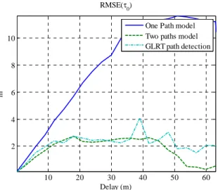
We try to give several explanations to that. First of all, the Van was situated at 5m of the wall and thus, we could expect a multipath with a relative delay of 0.02Chips. The data was sampled at the rate of 2.5 MHz and due to the anti aliasing filter, the signal bandwidth is around 2MHz. With such a bandwidth, we can not expect to detect or estimate shorter delay MP. To illustrate this idea, a simulation has been done and we plot on Figure 14. the RMSE of the time-delay estimation of the LOS with respect to the relative delay of one static MP. We plot the RMSE for the one path, two paths SAGE algorithms in the following scenario: θ0 = 60°, φ0 = 131°, υ0 = 100 Hz, θ1 = 30°, φ1 = 110°, υ1 = 105 Hz, relative power=-3dB. We also use the Generalized Likelihood Ratio Test [10] (GLRT) to estimate the number of paths in order to get the optimum likelihood estimation of the delay. In Figure 14. we can see that the performances between the different models (one, two paths or estimation of the number of paths)

are quite similar when the relative delay is around 5m. Moreover, we should note that the multipath conditions are worst in the simulated scenario than in the experimental condition (no polarization attenuation, multipath in phase …).

10 20 30 40 50 60 2 4 6 8 10 Delay (m) m RMSE(τ₀)

One Path model Two paths model GLRT path detection

Figure 14. Example of the Cross correlation function

Finally, if we want to be able to detect and measure the impact of strong multipath, other measurements campaigns should be done farther from the wall. If we put the array at 30m for example, we can expect to detect multipath with a relative delay of 0.1Chips. Such a multipath can lead to a strong positioning error in the case of one path maximum likelihood estimators (DLL), and SAGE approach may provide a real improvement in the time delay estimation of the LOS.

Moreover, we can see in the Figure 8. and Figure 9. that calibration errors are still present. However, we assume in the maximum likelihood formulation that the signal is perfectly calibrated. Thus, we should improve the performance by proposing other formulation of the maximum likelihood estimation (unstructured model as in [11] for example) or by including calibration errors in the model.

VIII. CONCLUSION

In this paper, we have compared the performance of the signal processing techniques which can be used for multipath mitigation in GNSS receivers with an antenna array: (i) SAGE algorithm and (ii) adaptive antenna algorithms based on digital beamforming and direction of arrival estimation. Simulations show that SAGE provides a real improvement in the mitigating the multipath effect due to the effective combining of all available information about the arriving signals in different domains (delay, Doppler and space domain) and achieving accurate estimation of the parameters of the line-of-sight signal, i.e. the signal of interest. The improvement is especially noticeable for highly correlated multipath echoes. The results for post-processing of real-world data presented in

the paper refer to a specific signal scenario with very short relative excess delay of the multipath echo (5m). Because of weak multipath effect occurred at such excess delays, these results cannot fully demonstrate the advantages of SAGE technique. Thus, other measurement campaign should be done in order to fill the gap between the theory and praxis. Also, another formulation of the maximum likelihood estimation problem can be used in order to make SAGE algorithm more robust in the presence of calibration errors.

REFERENCES

[1] A. J. Van Dierendonck, P. Fenton, and T. Ford, "Theory and Performance of Narrow Correlator Spacing in a GPS Receiver", Journal of the institute of navigation, vol.39, n°3, Fall 1992.

[2] R. D. J. Van Nee, J. Siereveld, P. C. Fenton, and B. R Townsend, "The Multipath Estimating Delay Lock Loop: Approaching Theoretical Accuracy Limits", IEEE Position, Location and Navigation Symposium, Las Vegas, Nevada, April U-15, 1994.

[3] A. Konovaltsev, F. Antreich, A. Hornbostel,

"Performance Assessment of Antenna Array Algorithms for multipath and Interference Mitigation", Proc. ESA Workshop on GNSS Signals 2007, ESTEC, Apr. 2007.

[4] B. H. Fleury, M. Tschudin, R. Heddergott, D. Dahlhaus, and K. I. Perdensen, "Channel Parameters Estimation in Mobil Radio Environments Using SAGE algorithm", IEEE Journal on Selected Areas in Communications, vol.17, n°3, March 1999.

[5] F. Antreich, J.A. Nossek, and W. Utschick, "Maximum likelihood delay estimation in a navigation receiver for aeronautical applications", Aerospace Science and Technology, vol.12, pp.256–267, 2008.

[6] Key Strategies for Safety-of-Life Receiver Development, Manuel Cuntz, Holmer Denks,Lukasz A. Greda, Marcos V.T. Heckler, Achim Hornbostel, Andriy Konovaltsev, Georg Buchner, Achim Dreher, Michael Meurer

[7] Antenna and RF Front End Calibration in a GNSS Array Receiver, Andriy Konovaltsev, Manuel Cuntz, Lukasz A. Greda, Marcos V.T. Heckler, Michael Meurer, IMWS 2010. [8] H. L. Van Trees , "Optimum array processing Array Processing, Part IV of Detection, Estimation, and Modulation Theory", WILEY-INTERSCIENCE 2002.

[9] M. Haardt, M.D. Zoltowski, and C.P. Mathews, "ESPRIT and Closed-Form 2D Angle Estimation with Planar

Arrays," in Digital Signal Processing Handbook, Section XII-63, CRC Press, Boca Raton, FL, 1998

[10] Akaike, H, "Information theory and an extension of the maximum likelihood principle", In Petrov, B. and Csaki, F., editors, 2nd International Symposium on Information theory, pp 267-281, Budapest, Hungary.

[11]. Felix Antreich, Josef A. Nossek, Gonzalo Seco, and A. Lee Swindlehurst, "Time-delay estimation applying the extended invariance principle with a polynomial rooting approach"