State estimation problems in heat transfer

HAL Id: hal-01688411

https://hal.archives-ouvertes.fr/hal-01688411

Submitted on 31 Oct 2019

HAL is a multi-disciplinary open access

archive for the deposit and dissemination of

sci-entific research documents, whether they are

pub-lished or not. The documents may come from

teaching and research institutions in France or

abroad, or from public or private research centers.

L’archive ouverte pluridisciplinaire HAL, est

destinée au dépôt et à la diffusion de documents

scientifiques de niveau recherche, publiés ou non,

émanant des établissements d’enseignement et de

recherche français ou étrangers, des laboratoires

publics ou privés.

Helcio Orlande, Marcelo Colaco, George Dulikravich, Flavio Vianna,

Wellington Silva, Henrique Fonseca, Olivier Fudym

To cite this version:

Helcio Orlande, Marcelo Colaco, George Dulikravich, Flavio Vianna, Wellington Silva, et al.. State

estimation problems in heat transfer. International Journal for Uncertainty Quantification, Begell

House Publishers, 2012, 2 (3), pp.239-258. �10.1615/Int.J.UncertaintyQuantification.2012003582�.

�hal-01688411�

STATE ESTIMATION PROBLEMS IN HEAT TRANSFER

Helcio Orlande,

_{Marcelo Colaço,}

_{George Dulikravich,}

_{Flavio Vianna,}

Wellington da Silva,

_{Henrique Fonseca,}

_{& Olivier Fudym}

1

_{Department of Mechanical Engineering, Politecnica/COPPE, Federal University of Rio de}

Janeiro, UFRJ, Cid. Universitaria, Cx. Postal: 68503, Rio de Janeiro, RJ, 21941-972, Brazil

2

_{Department of Mechanical and Materials Engineering, Florida International University, 10555}

West Flagler Street, EC 3462, Miami, FL 33174

3

_{Department of Subsea Technology, Petrobras Research and Development Center—CENPES,}

Av. Horácio Macedo, 950, Cidade Universitaria, Ilha do Fundao, 21941-915, Rio de Janeiro, RJ,

Brazil

4

_{Universite de Toulouse, Mines Albi, CNRS, Centre RAPSODEE, Campus Jarlard, F-81013}

Albi cedex 09, France

Original Manuscript Submitted: 10/14/2011; Final Draft Received: 03/28/2012

The objective of this paper is to introduce applications of Bayesian filters to state estimation problems in heat transfer. A brief description of state estimation problems within the Bayesian framework is presented. The Kalman filter, as well as the following algorithms of the particle filter: sampling importance resampling and auxiliary sampling importance resampling, are discussed and applied to practical problems in heat transfer.

KEY WORDS: Kalman filter, inverse problems, particle filters, fluid mechanics, heat transfer

1. INTRODUCTION

State estimation problems, also designated as nonstationary inverse problems [1], are of great interest in innumerable practical applications. In this kind of problem, the available measured data are used together with prior knowledge about the physical phenomena and the measuring devices in order to sequentially produce estimates of the desired dynamic variables. This is accomplished in such a manner that the error is minimized statistically [2].

State estimation problems are solved with the so-called Bayesian filters [1, 2]. In the Bayesian approach to statis-tics, an attempt is made to utilize all available information in order to reduce the amount of uncertainty present in an inferential or decision-making problem. As new information is obtained, it is combined with previous information to form the basis for statistical procedures. The formal mechanism used to combine the new information with the previously available information is known as Bayes’ theorem [1, 3].

The most widely known Bayesian filter method is the Kalman filter [1, 2, 4–9]. However, the application of the Kalman filter is limited to linear models with additive Gaussian noises. Extensions of the Kalman filter were developed in the past for less restrictive cases [1, 3, 6–8]. Similarly, Monte Carlo methods have been developed in order to represent the posterior density in terms of random samples and associated weights. Such Monte Carlo methods, usually denoted as particle filters, among other designations found in the literature, do not require the restrictive hypotheses of the Kalman filter. Hence, particle filters can be applied to nonlinear models with non-Gaussian errors [1, 4, 8–18]. In this paper, we present the application of the Kalman filter and of two different algorithms of the Particle filter, namely the sampling importance resampling and auxiliary sampling importance resampling [1–18], to state estimation

problems in heat transfer [19–30]. Before focusing on the applications of interest, the state estimation problem is defined and the Kalman and particle filters are described.

2. STATE ESTIMATION PROBLEM

In order to define the state estimation problem, consider a model for the evolution of the vector x in the following form [9]:

xk= fk(xk−1, vk−1) (1)

where the subscript k = 1, 2, . . ., denotes a time instant tkin a dynamic problem. The vector x ∈ Rnxis called the

state vector and contains the variables to be dynamically estimated. This vector advances in accordance with the state evolution model given by Eq. (1), where f is, in the general case, a nonlinear function of the state variables x and of the state noise vector v ∈ Rnv_.

Consider also that measurements zk ∈ Rnz are available at tk, k = 1, 2, . . .. The measurements are related to the

state variables x through the general, possibly nonlinear, function h in the form

zk = hk(xk, nk) (2)

where n ∈ Rnn_{is the measurement noise. Equation (2) is referred to as the observation (measurement) model.}

The state estimation problem aims at obtaining information about xkbased on the state evolution model (1) and

on the measurements z1:k= zi, i = 1, . . . , k given by the observation model (2) [1–18].

The evolution-observation model given by Eqs. (1) and (2) are based on the following assumptions [1, 4]: 1. The sequence xkfor k = 1, 2, . . ., is a Markovian process; that is,

π(xk|x0, x1, . . . , xk−1) = π(xk|xk−1) (3)

2. The sequence zkfor k = 1, 2, . . ., is a Markovian process with respect to the history of xk; that is,

π(zk|x0, x1, . . . , xk) = π(zk|xk) (4)

3. The sequence xkdepends on the past observations only through its own history; that is,

π(xk|xk−1, z1:k−1) = π(xk|xk−1) (5)

where π(a|b) denotes the conditional probability of a when b is given.

In addition, for the evolution-observation model given by Eqs. (1) and (2) it is assumed that for i 6= j the noise vectors viand vj, as well as ni and nj, are mutually independent and also mutually independent of the initial state x0. The vectors viand njare also mutually independent for all i and j [1].

Different problems can be considered with the above evolution-observation model, namely [1]: 1. The prediction problem, concerned with the determination of π(xk|z1:k−1);

2. The filtering problem, concerned with the determination of π(xk|z1:k);

3. The fixed-lag smoothing problem, concerned with the determination of π(xk|z1:k+p), where p ≥ 1 is the fixed

lag;

4. The whole-domain smoothing problem, concerned with the determination of π(xk|z1:K), where z1:K = zi, i = 1, . . . , K is the complete sequence of measurements.

This paper deals only with the filtering problem. By assuming that π(x0|z0) = π(x0) is available, the posterior

probability density π(xk|z1:k) is then obtained with Bayesian filters in two steps [1–18]: prediction and update, as

illustrated in Fig. 1. The Kalman filter and the particle filter used in this work are discussed in Sections 3 and 4, respectively.

FIG. 1: Prediction and update steps for the Bayesian filter [1].

3. THE KALMAN FILTER

For the application of the Kalman filter, it is assumed that the evolution and observation models given by Eqs. (1) and (2) are linear. Also, it is assumed that the noises in such models are Gaussian, with known means and covariances, and that they are additive. Therefore, the posterior density π(xk|z1:k) at tk, k = 1, 2, . . . is Gaussian and the Kalman filter

results in the optimal solution to the state estimation problem; that is, the posterior density is calculated exactly [1, 2, 4–9]. With the foregoing hypotheses, the evolution and observation models can be written respectively as

xk = Fkxk−1+ vk−1 (6)

zk = Hkxk+ nk (7)

where F and H are known matrices for the linear evolutions of the state x and of the observation z, respectively. By assuming that the noises v and n have zero means and covariance matrices Q and R, respectively, the prediction and update steps of the Kalman filter for Eqs. (6) and (7) are given by [1, 2, 4–9]:

Prediction: x− k = Fkˆxk−1 (8) P−_k = FkPk−1FTk + Qk (9) Update: Kk = P−kHTk(HkP−kHTk + Rk)−1 (10) ˆ xk = x−_k + Kk(zk− Hkx−_k) (11) Pk = (I − KkHk)P−k (12)

The matrix K is called Kalman’s gain matrix. Note above that, after predicting the state variable x and its covari-ance matrix P with Eqs. (8) and (9), a posteriori estimates for such quantities are obtained in the update step with the utilization of the measurements z.

For other cases in which the hypotheses of linear Gaussian evolution-observation models are not valid, the use of the Kalman filter does not result in optimal solutions because the posterior density is not analytic. The application of Monte Carlo techniques then appears as the most general and robust approach to nonlinear and/or non-Gaussian distributions. This is the case despite the availability of the so-called extended Kalman filter and its variations, which generally involves a linearization of the problem [1, 4, 8–18]. A Monte Carlo filter is described Section 4.

4. PARTICLE FILTER

The particle filter method [1, 4, 8–18] is a Monte Carlo technique for the solution of the state estimation problem. The particle filter, is also known as the bootstrap filter, condensation algorithm, interacting particle approximations, survival of the fittest and sequential Monte Carlo method [9]. The key idea is to represent the required posterior density function by a set of random samples (particles) with associated weights and to compute the estimates based on these samples and weights. As the number of samples becomes very large, this Monte Carlo characterization becomes an equivalent representation of the posterior probability function and the solution approaches the optimal Bayesian estimate. The particle filter algorithms generally make use of an importance density, which is a density proposed to represent another one that cannot be exactly computed, that is, the sought posterior density in the present case. Then, samples are drawn from the importance density instead of the actual density.

Let xi_0:k, i = 0, . . . , N be the particles with associated weights wi

k, i = 0, . . . , N and x0:k = xj, j = 0, . . . , k

be the set of all state variables up to tk, where N is the number of particles. The weights are normalized so that N

P i=1w

i

k= 1. Then, the posterior density at tkcan be discretely approximated by [1, 4, 8–18]:

π(x0:k|z1:k) ≈ N X i=1 wi kδ(x0:k− xi0:k) (13)

where δ(.) is the Dirac δ function. Similarly, its marginal distribution, which is of interest for the filtering problem, can be approximated by π(xk|z1:k) ≈ N X i=1 wi kδ(xk− xik) (14)

with weights computed from [9]:

wi k ∝ wk−1i π(zk|xik) π(xik|xik−1) q(xi k|xik−1, zk) (15)

where, for the derivation of Eq. (15), the importance density q(xi_k|xi

1:k−1, z1:k) was assumed to be given by q(xik|xik−1, zk); that is, it depends only on xik−1and zk, instead of the whole histories of each particle and of the measurements.

The optimal choice of the importance density, which minimizes the variance of the importance weights conditioned upon xi_k−1and zk, is given by q(xik|xik−1, zk) = π(xik|xik−1, zk). However, for most practical problems, this optimal

choice is not analytically tractable and a suboptimal importance density is taken as the transitional prior; that is, q(xi

k|xik−1, zk) = π(xik|xik−1) [9], so that Eq. (15) reduces to

wi

k ∝ wik−1π(zk|xik) (16)

The sequential application of the particle filter might result in the degeneracy phenomenon, where after a few states all but very few particles have negligible weight [1, 4, 8–18]. The degeneracy implies that a large computational effort is devoted to updating particles whose contribution to the approximation of the posterior density function is almost zero. This problem can be overcome with a resampling step in the application of the particle filter. Resampling involves a mapping of the random measure {xi_k, wi_k} into {xi∗_k, N−1} with uniform weights; it deals with the elimination of particles originally with low weights and the replication of particles with high weights. Resampling can be performed if the number of effective particles (particles with large weights) falls below a certain threshold number [1, 4, 8–18].

Alternatively, resampling can also be applied indistinctively at every instant tk, as in the SIR algorithm described

in [8, 9]. Such algorithm can be summarized in the steps presented in Table 1, as applied to the system evolution from tk−1to tk[8, 9].

In the first step of the SIR algorithm presented in Table 1, it should be noted that the weights are given directly by the likelihood function π(zk|xik). Such is the case because in this algorithm the resampling step is applied at each

time instant and then the weights wi_k−1are uniform [see Eq. (16)].

Although the resampling step reduces the effects of the degeneracy problem, it may lead to a loss of diversity and the resultant sample may contain many repeated particles. Hence, despite the fact that in the SIR algorithm the weights are easily computed and the importance density can be easily sampled, the particles may experience a fast loss of diversity. Indeed, this problem, known as sample impoverishment, can be severe in the case of small state evolution noise [1, 8, 9, 18]. In addition, in the SIR algorithm the state space is explored without the information conveyed by the measurements; that is, the particles at each time instant are generated through the sole application of the transition prior π(xi_k|xi_k−1) (see step 1 in Table 1). With the ASIR algorithm, an attempt is made to overcome these drawbacks by performing the resampling step at time tk−1, with the available measurement at time tk [9]. The resampling is

based on some point estimate µi_k that characterizes π(xk|xik−1), which can be the mean of π(xk|xik−1) or simply a

sample of π(xk|xik−1). If the state evolution model noise is small, then π(xk|xik−1) is generally well characterized by µi

k, so that the weights wki are more even and the ASIR algorithm is less sensitive to outliers than the SIR algorithm.

On the other hand, if the state evolution model noise is large, then the single point estimate µi_k in the state space may not characterize well π(xk|xik−1) and the ASIR algorithm may not be as effective as the SIR algorithm. The

ASIR algorithm can be summarized in the steps presented in Table 2, as applied to the system evolution from tk−1to

tk[8, 9].

A drawback of the particle filter is related to the large computational costs due to the Monte Carlo method, which may not allow its application to be used for complicated physical problems. On the other hand, more involved algo-rithms than the ones presented above have been developed [9, 18], which can reduce the number of particles required for an appropriate representation of the posterior density, thus resulting in the reduction of associated computational times, especially when associated with parallel computing techniques. In addition, the use of reduced models or response surfaces for the solution of the direct problem appear as promising approaches for the reduction of the computational time, thus enabling the use of sampling methods for more involved cases.

TABLE 1: Sampling importance resampling algorithm [8, 9] Step 1

For i = 1, · · · , N draw new particles xi_kfrom the prior density π¡xk ¯ ¯xi

k−1 ¢

and then use the likelihood density to calculate the corresponding weights w_ki = π¡zk

¯ ¯xi k ¢ . Step 2

Calculate the total weight Tw = N P i=1

wi

kand then normalize the particle weights; that is,

for i = 1, · · · , N letw_ki = T_w−1w_ki

Step 3

Resample the particles as follows:

Construct the cumulative sum of weights (CSW) by computing ci = ci−1 + wikfor

i = 1, · · · , N , with c0 = 0.

Let i = 1 and draw a starting point u1from the uniform distribution U

£

0, N−1¤

For j = 1, · · · , N

Move along the CSW by making uj = u1 + N−1(j − 1)

While uj > cimake i = i + 1.

Assign sample xj_k = xi k

TABLE 2: Auxiliary sampling importance resampling algorithm [8, 9] Step 1

For i = 1, . . . , N draw new particles xi_kfrom the prior density π(xk|xik−1) and then

calculate some characterization µi_kof xk, given xik−1. Then use the likelihood density to

calculate the corresponding weights wi_k = π(zk|µik)wk−1i Step 2

Calculate the total weight t = Σiwikand then normalize the particle weights; that is, for

i = 1, . . . , N let wi

k= t−1wik Step 3

Resample the particles as follows:

Construct the cumulative sum of weights (CSW) by computing ci = ci−1+ wikfor

i = 1, . . . , N , with c0= 0

Let i = 1 and draw a starting point u1from the uniform distribution U [0, N−1]

For j = 1, . . . , N

Move along the CSW by making uj = u1+ N−1(j − 1)

While uj> cimake i = i + 1

Assign sample xj_k= xi_k Assign sample w_kj = N−1

Assign parent ij= i Step 4

For j = 1, . . . , N draw particles xj_kfrom the prior density π(xk|xijk−1), using the parent

ij_{, and then use the likelihood density to calculate the correspondent weights}

wj_k= π(zk|xjk)/π(zk|µijk) Step 5

Calculate the total weight t = Σjwkjand then normalize the particle weights; that is, for

j = 1, . . . , N let w_kj = t−1_wj k

5. APPLICATIONS

In this section, we apply the Bayesian filters described above to state estimation problems in heat transfer that have been recently addressed by our group. These problems include: (i) the estimation of a position-dependent transient heat source in a plate [26]; (ii) the estimation of the temperature field in oil pipelines [29]; (iii) the estimation of a transient line source and the solidification front in a phase-change problem [24]; and (iv) the estimation of the transient boundary heat flux in a natural convection problem [25]. For all cases, simulated temperature measurements were used in the inverse analysis. The problems examined are described below, and the results obtained are then discussed.

5.1 Estimation of a Position-Dependent Transient Heat Source in a Plate [26]

We present here the estimation of a transient heat source term that also varies spatially by using the Kalman filter. The physical problem involves two-dimensional transient heat conduction in a plate, with constant thermal conductivity and volumetric heat capacity. Lateral boundaries are supposed to be insulated. This situation can be found when performing experiments on a thin plate, with partial lumping across the plate. Both internal transient heat generation and constant convective heat losses are taken into account. The mathematical formulation for this problem is given by

C∂T ∂t = ∂ ∂x µ k∂T ∂x ¶ + ∂ ∂y µ k∂T ∂y ¶ −h e(T − T∞) + g(x, y, t) e in 0 < x < L, 0 < y < L, for t > 0 (17) ∂T ∂x = 0 at x = 0 and x = L, for t > 0 (18)

∂T

∂y = 0 at y = 0 and y = L, for t > 0 (19)

T = T0 for t = 0, at 0 < x < L and 0 < y < L (20)

where C and k are the volumetric heat capacity and thermal conductivity of the plate material, respectively, h is the heat transfer coefficient at the surface of the plate, L and e are the width and thickness of the plate, respectively, and g(x, y, t) is the sought volumetric heat source term. We assume that transient temperature measurements are available at several positions (x, y) at the plate surface. The temperature measurements are supposedly taken with an infrared camera. Such a measurement technique is quite powerful because it can provide accurate non-intrusive measurements, with fine spatial resolutions and at large frequencies.

For the identification of the spatial and time varying heat source, g(x, y, t), we apply the so-called nodal strategy, which is briefly described below. Such a strategy makes use of the nonconservative form of Eq. (17), which is rewritten as follows:

∂T ∂t = a∇

2_{T − H(T − T}

∞) + G(x, y, t) (21)

where H = h/eC, G(x, y, t) = g(x, y, t)/eC, and a = k/C is the thermal diffusivity of the material. An explicit discretization of Eq. (21) by using finite differences results in

Y_i,jk+1= Lk

i,jaki,j− ∆t(Ti,jk − T∞)H + ∆tGki,j (22)

where the subscripts (i, j) denotes the finite-difference node at xi = i∆x, i = 1, . . . , I and yi = j∆y, j = 1, . . . , J

and the superscript k denotes the time tk= k∆t, k = 1, . . . , K. The other quantities appearing in Eq. (22) are given

by Y_ik+1= T_ik+1− Tik (23) Lk i,j= ∆t " Tk

i−1,j− 2Ti,jk + Ti+1,jk

(∆x)2 +

Tk

i,j−1− 2Ti,jk + Ti,j+1k (∆y)2

#

(24)

Equation (23) defines the forward temperature difference in time, while Eq. (24) approximates the Laplacian of temperature at time tkand node (i, j).

Equation (22) is now rewritten in the form of a state evolution model, for the application of the Kalman filter, by reordering sequentially all the nodes (i, j) with the index m = 1, . . . , M , where M = IJ . Then, Eq. (22) becomes

Tk+1_{= T}k_{+ J}k_Pk ₍₂₅₎ where Jk₌      Lk 1 −∆t(T1k− T∞) ∆t 0 0 0 0 0 Lk 2 −∆t(T2k− T∞) .. . 0 · · · ∆t · · · 0 0 Lk M −∆t(TMk − T∞) ∆t      (26) Tk ₌      Tk 1 Tk 2 .. . Tk M      (27)

Pk₌                          ak 1 Hk 1 Gk 1       ak 2 Hk 2 Gk 2    .. .    ak M Hk M Gk M                          (28)

The vector of parameters defined by Eq. (28) contains at each node, a, which is the thermal diffusivity, H, which is the heat transfer convective coefficient divided by the heat capacity and thickness of the plate, and G, which is the local heat source divided by the heat capacity and thickness of the plate.

The sensitivity matrix defined by Eq. (26) is a function of the temperature field and thus depends on the unknown parameters. This fact would yield a nonlinear estimation procedure. One way to circumvent this problem is to use a predictive error model, where the measured data are directly passed to the model. Hence, with the spatial resolution and frequency of measurements made available by infrared cameras, the sensitivity matrix can be approximately computed with the measurements and the estimation problem becomes linear.

In order to demonstrate the Kalman filter approach for estimating the transient heat sourc term Gk_m, we make use of the following test case involving a slab with thickness e = 2 × 10−3m. The slab is composed of a material with thermal properties k = 10 W m−1K−1and C = 3.76 × 106J m−3K−1, subjected to heat source that varies in time in accordance with a double step function. In order to avoid the inverse crime of using the same direct solution for the generation of the simulated measurements and for the solution of the inverse problem, a finite-volume solution was developed that yields the simulated exact data. For the solution of the inverse problem, the slab was discretized with I = J = 60 internal nodes and 70 time steps. The values of the source term Gk

mat each of these volumes and times

steps were then estimated. The final time was taken as 1.4 s, and the time step was chosen as 0.02 s. The spatial grid was chosen as ∆x = ∆y = 500µ m, so that the width and length of the plate were 0.03 m. The heat transfer coefficient was assumed to have a uniform value of 5 W m−2 K−1 over the plate, throughout the duration of the experiment. The plate was assumed to be initially at the uniform temperature of 20◦C. The measured variables are assumed to be the transient temperatures inside the medium at the finite volume nodes. The errors in the simulated measured temperatures are additive, uncorrelated, normally distributed, with zero mean, and constant standard deviation of 0.2◦C, which is typical of measurements taken with an infrared camera. A random walk model was used for the evolution of the source term Gk_m.

Figures 2 and 3 present the spatial variation of the heat source term used to generate the simulated measurements and its estimation with the Kalman filter, respectively. The transient variation of the heat source term at a specific discretization node is presented in Fig. 4. These figures show that the Kalman filter can very accurately estimate the transient variation of the heat source term, although some lagging is observed near the discontinuities in Fig. 4.

5.2 Estimation of the Temperature field in Oil Pipelines [29]

Flow assurance in the petroleum industry is one of the challenges for the development of subsea field layouts due to a combination of factors, involving among others, the dynamic nature of the produced multiphase fluids, high internal hydrostatic pressures, and low external environmental temperatures. Thermal management of equipment and pipeline systems are of great importance for the prediction and prevention of solid deposits. In general, the subsea systems are designed to transport the produced fluids without experiencing significant heat losses to the surroundings. Recently, new technologies have emerged for monitoring and controlling critical parameters associated with the flow assurance.

FIG. 2: Exact spatial variation of the heat source.

FIG. 3: Estimated spatial variation of the heat source.

One of these technologies is based on the use of optical fibers, for the measurement of the temperature profile along the pipeline.

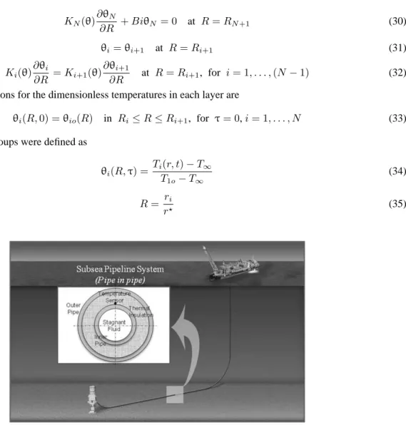
This example aims at the application of the SIR algorithm presented above, for the accurate prediction of the unsteady temperature field of the produced fluid inside a typical multilayered pipeline, during shutdown periods. The physical problem involves a typical pipeline cross section. It is represented by a circular domain filled by the stagnant petroleum fluid, which is bounded by a multilayered wall, such as in a pipe-in-pipe system (see Fig. 5).

The dimensionless mathematical formulation of this heat conduction problem in cylindrical coordinates is given by Pi(θ)Ci(θ)∂θi(R, τ) ∂τ = 1 R ∂ ∂R · RKi(θ)∂θi(R, τ) ∂R ¸ in Ri< R < Ri+1, for τ > 0, i = 1, . . . , N (29)

where θi is the dimensionless temperature, Ki is the dimensionless thermal conductivity, Pi is the dimensionless

density, and Ciis dimensionless specific heat in the ith layer. The inner and outer dimensionless radius of the ith layer

are Riand Ri+1, respectively, where R1corresponds to the centerline.

Equation (29) is subjected to the following boundary and interface conditions: KN(θ)∂θN ∂R + BiθN = 0 at R = RN +1 (30) θi= θi+1 at R = Ri+1 (31) Ki(θ)∂θi ∂R = Ki+1(θ) ∂θi+1 ∂R at R = Ri+1, for i = 1, . . . , (N − 1) (32) The initial conditions for the dimensionless temperatures in each layer are

θi(R, 0) = θio(R) in Ri≤ R ≤ Ri+1, for τ = 0, i = 1, . . . , N (33)

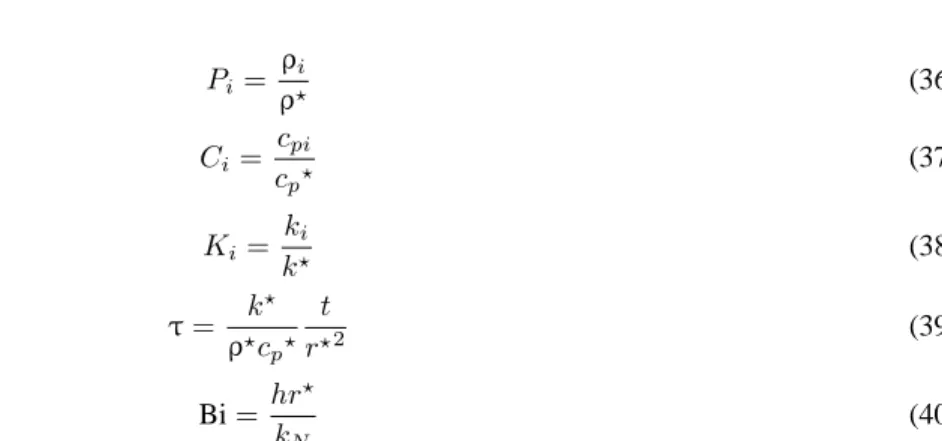
Dimensionless groups were defined as

θi(R, τ) = Ti(r, t) − T∞ T1o− T∞ (34) R = ri r? (35)

Pi= ρi ρ? (36) Ci= cpi cp? (37) Ki= ki k? (38) τ = k ? ρ?_cp? t r?2 (39) Bi = hr ? kN (40)

Here, T∞ is the surrounding environment temperature, r? is the external radius, T1o is the uniform initial fluid

temperature, k?is the reference thermal conductivity, ρ?is the reference density, c?_pis the reference specific heat, and h is the heat transfer coefficient at the outer surface of the pipeline.

For the test cases presented below, we consider the pipe-in-pipe to be made of an inner steel pipe with internal and external diameters of 0.2 m and 0.25 m, respectively. The outer pipe is also made of steel, with internal and external diameters of 0.35 and 0.40 m, respectively. The thermophysical properties of steel are assumed as constant. The annular space between the two concentric pipes is assumed to be filled with a thermal insulator with constant thermophysical properties, approximating those for polypropylene. The stagnant petroleum fluid inside the inner pipe has temperature-dependent properties, so that the state estimation problem is nonlinear.

The dimensionless temperature field in the pipe in pipe at a specific time is shown by the contour plot in Fig. 5. White circles in Fig. 6 are used on purpose to separate the spatial domains containing the stagnant fluid, the inner steel pipe, the thermal insulation, and the outer steel pipe.

The simulated temperature measurements used here are supposed to be taken at the outer surface of the inner pipe; that is, at r = 0.125 m. The measurement errors are assumed to be additive, Gaussian, uncorrelated, with zero mean, and a constant standard deviation of 2◦C. Such a standard deviation is characteristic of measurement systems used for the present application. Errors in the evolution model are also supposed to be additive, Gaussian, uncorrelated, with zero mean, and constant standard deviation of 4◦C. For the results presented below, 200 particles were used in the SIR algorithm of the particle filter method presented in Table 1. Numerical experiments revealed that such number of particles would be sufficient to represent the posterior distribution of the predicted states.

The mean values predicted for the dimensionless temperature field in the pipe-in-pipe system are presented in Fig. 7, for the same dimensionless time of Fig. 6. A comparison of Figs. 6 and 7 reveals that the particle filter method

FIG. 7: Predicted dimensionless temperature distribution.

is capable of very accurately predicting the temperature field in the pipe-in-pipe system, even when the evolution model errors are large.

The accuracy of the particle filter method, as applied to the prediction of the temperature field in the pipe-in-pipe system by using one single measurement point, can also be ascertained through the analysis of the estimated standard deviation of the predicted states. Figure 8 presents the contour plots of the estimated standard deviations, corresponding to the predictions presented in Fig. 7. Note that the standard deviations are relatively small as compared to the values of the predicted temperatures. Also, the largest standard deviations are generally observed in the stagnant fluid region. The smallest values of the standard deviation are found in the internal and external pipes, as a result of the small temperature gradients in these regions.

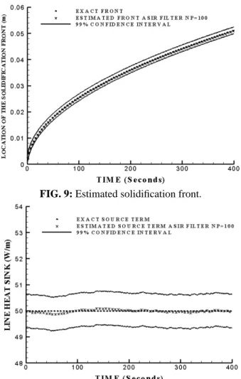
5.3 Estimation of a Transient Line Source and the Solidification Front in a Phase Change Problem [24]

The main objective of this nonlinear state estimation problem is to compare the performance of the SIR and the ASIR algorithms. The physical problem analyzed consists of a one-dimensional transient solidification problem in a

infinite medium in cylindrical coordinates. Initially, the entire medium is at a uniform temperature in the liquid phase and, at the initial time a heat sink is applied at r = 0. The material then starts to solidify at r = 0, and a solidification front moves away from the origin. The physical properties of liquid and solid phases are assumed constant. The material undergoing solidification is assumed to be a pure substance, so that phase change occurs at the temperature Tm. Transient temperature measurements taken at one single point inside the solidifying medium are used to estimate

the location of the solidification front, as well as the intensity of a line heat sink. The mathematical formulation for the solid phase is given as

1 r ∂ ∂r · r∂Ts(r, t) ∂r ¸ = 1 αs ∂Ts(r, t) ∂t in 0 < r < S(t) and t > 0 (41) and for the liquid phase as

1 r ∂ ∂r · r∂Tl(r, t) ∂r ¸ = 1 αl ∂Tl(r, t) ∂t in S(t) < r < ∞ and t > 0 (42) Tl(r, t) → Ti in r → ∞ and t > 0 (43) Tl= Ti at t = 0 and r > 0 (44)

At the interface between liquid and solid phases, the following conditions must be satisfied:

Ts= Tl= Tm at r = S(t) and t > 0 (45) ks∂Ts ∂r − kl ∂Tl ∂r = ρL ∂S(t) ∂t at r = S(t) and t > 0 (46) and at the centerline the following condition is satisfied:

lim r→0 · 2πrks∂Ts ∂r ¸ = Q (47)

An analytical solution can be obtained for this physical problem, and it is given by [31]: Ts(r, t) = Tm+ Q 4πks · Ei µ −r2 4αst ¶ − Ei(−λ2) ¸ 0 < r < S(t) (48) Tl(r, t) = Ti− (Ti− Tm) Ei[(−λ2αs)/αl] · Ei µ −r2 4αst ¶¸ S(t) < r < ∞ (49) where the eigenvalues λ and the solidification front S(t) are given respectively by

Q 4πe −λ2 + kl(Ti− Tm) Ei[(−λ2αs)/αl] e(−λ2_αs)/αl = λ2_α sρL (50) S(t) = 2λ√αst (51)

In the above equations Tiis the uniform initial temperature, Tmis the melting temperature of the material, L is the

latent heat of solidification of the material, ρ is the density, and ksand klare the thermal conductivities of the solid

and liquid phases, respectively, αsand αlare the thermal diffusivities of the solid and liquid phases, respectively, and

Tlare temperatures of the solid and liquid phases, respectively, Q is the strength of the line heat sink, and Eidenotes

the exponential integral function.

The physical problem defined by Eqs. (41)–(47) was solved for the following data, corresponding to solidifying water: Ti = 25◦C, Tm= 0◦C, αs= 0.00118 m2/s, αl = 0.000146 m2/s, ks= 2.22 W/(m◦C), kl = 0.61 W/(m◦C), ρ = 997.1 kg/m3_{, L = 80 J/kg. The line heat sink was supposed to have a constant value of Q = 50 W/m. In this}

were uncorrelated, additive, Gaussian, with zero mean and constant standard deviation equal to 5% of the maximum temperature.

A random walk model was used for the evolution model of the unknown line heat sink, as given by Eq. (52), where the subscript k denotes the time instant tk. In Eq. (52), σ is the standard deviation for the line heat sink, taken

to be equal to 0.25 W/m, while ωk is a random variable with normal distribution, zero mean, and unitary standard

deviation. Equation (53) shows the evolution model for the solidification front, obtained by rewriting Eq. (51) in an appropriate form for the application of the particle filter algorithms presented above. Uncertainties in the evolution model for the solidification front were also taken into account, as additive, Gaussian, with zero mean, and standard deviation σs. In Eq. (53), ω?kis a random variable with normal distribution, zero mean, and unitary standard deviation

Qk = Qk−1+ σωk (52) S(tk) = S(tk−1) + 2λ √ αs( √ tk− √ tk−1) + σsω?k (53)

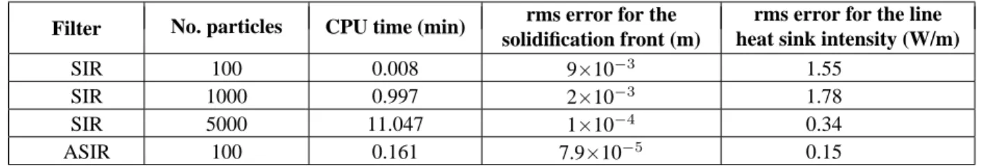
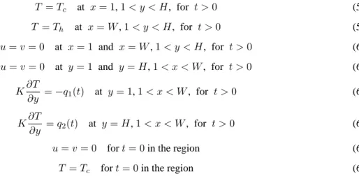
The two algorithms of the particle filter presented above were applied to the problem of estimating the transient line heat sink as well as the solidification front. Table 3 summarizes the cases examined as well as their results for CPU time and root-mean-square (rms) errors. Table 3 shows that the SIR algorithm resulted on computational times varying from 0.008 to 11.047 min, when the number of particles varied from 100 to 5000. Also, the variation of the rms in the estimation of the solidification front varied from 9×10−3to 1×10−4 m, by increasing the number of particles from 100 to 5000. On the other hand, by applying the ASIR algorithm with only 100 particles, the computational time was of 0.161 min, with an rms error of 2×10−5m in the estimation the solidification front. Also in Table 3, one can note that the rms error for recovering the line heat sink was much smaller for the ASIR algorithm than for SIR algorithm. Thus, the ASIR algorithm was capable of recovering the unknown quantities more accurately, faster, and with a much smaller number of particles than those required for the SIR algorithm.

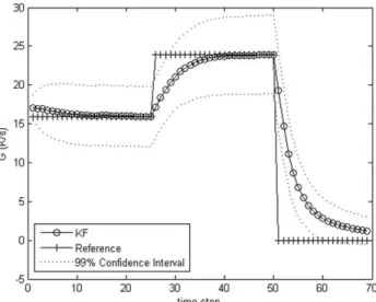
Figures 9 and 10 present the estimated solidification front and line heat sink intensity, respectively, obtained with the ASIR algorithm. Clearly, the estimated quantities are in excellent agreement with the exact ones. The 99% confidence intervals of the estimated solidification front and heat sink intensity are also presented in Figs. 9 and 10.

5.4 Estimation of the Transient Boundary Heat Flux in a Natural Convection Problem [25]

The physical problem now under examination involves the transient laminar natural convection of a fluid inside a two-dimensional square cavity. The fluid is initially at rest and at the uniform temperature Tc. At time zero, the bottom,

and top surfaces are subjected to time-dependent heat fluxes q1(t) and q2(t), respectively. The left and right surfaces

are subjected to constant temperatures Tcand Th, respectively. The fluid properties are assumed constant, except for

the density in the buoyancy term, where we consider Boussinesq’s approximation valid.

The mathematical formulation for this physical problem can be written in vector form in terms of the following conservation equation in the generalized Cartesian coordinates:

∂(ρϕ) ∂t + ∂(uρϕ) ∂x + ∂(vρϕ) ∂y = ∇ • (Γ ϕ_{∇ϕ) + S (54)}

TABLE 3: Computational time and rms errors

Filter No. particles CPU time (min) rms error for the

solidification front (m)

rms error for the line heat sink intensity (W/m)

SIR 100 0.008 9×10−3 1.55

SIR 1000 0.997 2×10−3 1.78

SIR 5000 11.047 1×10−4 0.34

FIG. 9: Estimated solidification front.

FIG. 10: stimated intensity of the heat sink.

The general conservation variable, as well as the diffusion coefficient and the source term for the mass, momentum, and energy conservation equations, are given in vector form, respectively, as

ϕ =     1 u(x, y, t) v(x, y, t) T (x, y, t)     (55) Γϕ=     0 0 0 0 0 µ 0 0 0 0 µ 0 0 0 0 K/Cp     (56) Sϕ=         0 −∂P (x, y, t) ∂x −∂P (x, y, t) ∂y − ρg{1 − β[T (x, y, t) − Tref]} 0         (57)

We note in the Eq. (57) that the positive y-axis in the physical domain was supposed to be aligned with the opposite direction of the gravitational acceleration vector. These equations are solved, subjected to the following boundary and initial conditions T = Tc at x = 1, 1 < y < H, for t > 0 (58) T = Th at x = W , 1 < y < H, for t > 0 (59) u = v = 0 at x = 1 and x = W , 1 < y < H, for t > 0 (60) u = v = 0 at y = 1 and y = H, 1 < x < W , for t > 0 (61) K∂T ∂y = −q1(t) at y = 1, 1 < x < W , for t > 0 (62) K∂T ∂y = q2(t) at y = H, 1 < x < W , for t > 0 (63) u = v = 0 for t = 0 in the region (64) T = Tc for t = 0 in the region (65)

We applied the ASIR algorithm to estimate the time-varying heat flux applied at the top wall of a square cavity, which is filled with air ρ = 1.19 kg/m3; K = 0.026 W/m K; cp= 1035.02 J/kg K; µ = 1.8×10−5 kg/m s; and β =

0.00341 K−1. The bottom wall of the cavity was kept thermally insulated, and the left and right walls were subjected to constant temperatures equal to 2 and 12◦C, respectively. The width and height of the cavity were equal to 0.046 m, which resulted in a Rayleigh (Ra) number equal to 105, where

Ra = ρ

2_C

pgβ(Th− Tc)W3

µK (66)

The state estimation problem consists thus in predicting the behavior of the state variable q2(t) at the top wall

of the cavity. However, because the heat flux affects the temperature field through the energy equation and also the mass and momentum equations through the buoyancy source term, Eqs. (54)–(65), the state vector is composed of the discretized heat flux q2(t), plus all velocity components and temperature values in each finite control volume inside

the cavity. Because of the amount of computational resources involved for the solution of this problem, we used a very course finite volume grid (11×11 volumes) to demonstrate the feasibility of the method. The total number of state variables is thus: 1 for the heat flux q2(t), 11×11 for the u component of the velocity field, 11×11 for the v

component of the velocity field, and 11×11 for the temperature T , resulting in 364 state variables.

The evolution model for the velocity and temperature values was given by the discretized form of mass, momen-tum, and energy equations, where the state noise was supposed to be additive, uncorrelated, Gaussian, with zero mean, and a standard deviation equal to 1% of the state variable values. For the heat flux q2(t), a random walk evolution

model was used.

For the observation model, we used simulated temperature measurements, where an experimental error with stan-dard deviation equal to 1% of the local value of the temperature was used. Such measurements were taken at the top and bottom walls of the cavity, in 11points equally spaced at each wall.

Figure 11 shows the estimated values of q2(t) with a linear exact variation, for two different number of particles

and two different measurement frequencies. The average values at each time are shown by the symbols with error bars corresponding to a 99% confidence interval. For the case with 10 particles and a measurement frequency of 1 Hz, there was an initial delay of almost 200 s in the estimation of such heat flux. However, when the number of particles was increased to 100, with the same measurement rate of 1 Hz, the particle filter was able to fully recover the unknown heat flux. When more particles were used, the uncertainty bars were more uniform during the whole time period examined, whereas for 10 particles there was a fluctuation in the associated uncertainty level of the estimated heat flux. One can also see in Fig. 11 that, when the frequency was increased from 1 to 10 Hz, the results became worse, with a larger fluctuation of the average heat flux and larger estimated uncertainties. This is due to the ill-posed

FIG. 11: Estimated heat flux with the linear profile.

character of the inverse problem, which becomes more sensitive to perturbations at higher measurement frequencies when sequential methods, such as the ones under examination, are utilized.

Figure 12 shows the exact and recovered temperature profiles, while Fig. 13 shows the exact and recovered stream-lines. One can note the excellent estimates of the temperature and velocity fields, despite the fact that the streamlines at 100 s, for the test case with 10 particles and a measurement frequency of 1 Hz, were not fully well captured. This is due to the initial delay of ∼200 s to estimate the heat flux in this case, as discussed above.

6. CONCLUSIONS

In this paper, we presented the application of the Kalman filter and two algorithms of the particle filter, to the solution of state estimation problems in heat transfer. The particle filter was coded in the form of the SIR algorithm and of the ASIR algorithm. The problems examined in this paper included: (i) The estimation of a position-dependent transient heat source in a plate, (ii) the estimation of the temperature field in oil pipelines, (iii) the estimation of a transient line source and the solidification front in a phase change problem, and (iv) the estimation of the transient boundary heat flux in a natural convection problem. For all cases, simulated temperature measurements were used in the inverse analysis.

For linear-Gaussian models, the Kalman filter results in optimal solutions, which can be obtained in smaller computational times than with the particle filters. On the other hand, in nonlinear and/or non-Gaussian models, the basic hypotheses required for the application of the Kalman filter are not valid. The particle filter thus appears in the literature as an accurate estimation technique of general use.

FIG. 12: Real and estimated temperature profiles with the linear heat flux variation.

FIG. 13: Real and estimated streamlines with the linear heat flux profile.

The two algorithms of the particle filter examined here were successfully applied to the solution of nonlinear state estimation problems. Such Monte Carlo techniques provided accurate estimation results, even for strict cases involving large errors in the evolution and observation models. However, numerical experiments revealed that a drastic reduction on the number of particles used to represent the posterior density function could be achieved by using the ASIR algorithm instead of the SIR algorithm. Therefore, the ASIR algorithm appears as a robust and efficient tool for complicated problems, such as the one dealing with natural convection examined above.

ACKNOWLEDGMENTS

The financial support provided by FAPERJ, CAPES, and CNPq, Brazilian agencies for the fostering of science, is greatly appreciated.

REFERENCES

1. Kaipio, J. and Somersalo, E., Statistical and Computational Inverse Problems, Applied Mathematical Sciences, Springer, Berlin, 2004.

2. Maybeck, P., Stochastic Models, Estimation and Control, Academic Press, New York, 1979.

3. Winkler, R., An Introduction to Bayesian Inference and Decision, Probabilistic Publishing, Gainsville, Florida, 2003. 4. Kaipio, J., Duncan, S., Seppanen, A., and Somersalo, E., Handbook of Process Imaging for Automatic Control, State

Estima-tion for Process Imaging, CRC Press, Boca Raton, FL, 2005.

5. Kalman, R., A new approach to linear filtering and prediction problems, ASME J. Basic Eng., 82:35–45, 1960. 6. Sorenson, H., Least-squares estimation: From Gauss to Kalman, IEEE Spectrum, 7:63–68, 1970.

7. Welch, G. and Bishop, G., An introduction to the Kalman filter, Tech. Rep. No. TR 95-041, University of North Carolina, 2006.

8. Arulampalam, S., Maskell, S., Gordon, N., and Clapp, T., A tutorial on particle filters for on-line non-linear/non-gaussian Bayesian tracking, IEEE Trans. Signal Process., 50:174–188, 2001.

9. Ristic, B., Arulampalam, S., and Gordon, N., Beyond the Kalman Filter, Artech House, Boston, 2004.

10. Doucet, A., Godsill, S., and Andrieu, C., On sequential Monte Carlo sampling methods for Bayesian filtering, Stat. Comput., 10:197–208, 2000.

11. Liu, J. and Chen, R., Sequential Monte Carlo methods for dynamical systems, J. Am. Stat. Assoc., 93:1032–1044, 1998. 12. Andrieu, C., Doucet, A., and Robert, C., Computational advances for and from Bayesian analysis, Stat. Sci., 19:118–127,

2004.

13. Johansen, A. and Doucet, A., A note on auxiliary particle filters, Stat. Probab. Lett., 78(12):1498–1504, 2008.

14. Carpenter, J., Clifford, P., and Fearnhead, P., An improved particle filter for non-linear problems, IEEE Proc. Part F, 146:2–7, 1999.

15. Moral, P. D., Doucet, A., and Jasra, A., Sequential Monte Carlo for Bayesian computation, Bayesian Stat., 8:1–34, 2007. 16. Moral, P. D., Doucet, A., and Jasra, A., Sequential Monte Carlo samplers, J. R. Stat. Soc., 68:411–436, 2006.

17. Andrieu, C., Doucet, A., Sumeetpal, S., and Tadic, V., Particle methods for charge detection, system identification and control,

Proc. of IEEE, 92:423–438, 2004.

18. Doucet, A., Freitas, N., and Gordon, N., Sequential Monte Carlo Methods in Practice, Springer, New York, 2001.

19. Kaipio, J. and Fox, C., The Bayesian framework for inverse problems in heat transfer, Heat Transfer Eng., 32:718–753, 2011. 20. Matsevityi, Y. and Multanovskii, A., An iterative filter for solution of the inverse heat conduction problem, J. Eng. Phys.,

35:1373–1378, 1978.

21. Matsevityi, Y. and Multanovskii, A., Pointwise identification of thermophysical chracteristics, J. Eng. Phys., 49:1392–1397, 1985.

22. Orlande, H. R. B., Dulikravich, G. S., and Colac¸o, M. J., Application of Bayesian filters to heat conduction problem, Interna-tional Conference on Eng. Optimization, Herskovits, J., ed., Rio de Janeiro, Brazil, June, 2008.

23. Silva, W. B., Orlande, H. R. B., and Colac¸o, M. J., Evaluation of Bayesian filters applied to heat conduction problems, Proc.

of 2nd International Conference on Engineering Optimization, Lisbon, Portugal, Sept., 2010.

24. Silva, W. B., Orlande, H. R. B., Colac¸o, M. J., and Fudym, O., Application of Bayesian filters to a one-dimensional solidifica-tion problem, Proc. of 21st Brazilian Congress of Mechanical Engineering, Natal, Brazil, Oct., 2011.

25. Colac¸o, M. J., Orlande, H. R. B., Silva, W. B., and Dulikravich, G. S., Application of a Bayesian filter to estimate unknown heat fluxes in a natural convection problem, ASME International Design Engineering Technical Conferences (IDETC/CIE)

and Computers and Information in Engineering Conference (CIE), Dennis, B. H. and Michopoulos, J., eds., ASME Paper No.

26. Fonseca, H., Orlande, H. R. B., Fudym, O., and Sepulveda, F., Kalman filtering for transient source term mapping from infrared images, Inverse Problems, Design And Optimization Symposium, Jo´co Pessoa, Brazil, Aug., 2010.

27. Vianna, F., Orlande, H. R. B., and Dulikravich, G. S., Optimal heating control to prevent solid deposits in pipelines, Proc. of

5th European Conference on Computational Fluid Dynamics—ECCOMAS CFD 2010, Lisbon, Portugal, June 2010.

28. Vianna, F., Orlande, H. R. B., and Dulikravich, G. S., Pipeline heating method based on optimal control and state estimation,

Proc. of 13th Brazilian Congress of Thermal Sciences and Engineering (ENCIT), Uberlndia, Brazil, Dec., 2010.

29. Vianna, F., Orlande, H. R. B., and Dulikravich, G. S., Temperature field prediction of a multilayered composite pipeline based on the particle filter method, Proc. of 14th International Heat Transfer Conference (IHTC), Paper No. IHTC14-22462, Washington, DC, Aug., 2010.

30. Vianna, F., Orlande, H. R. B., and Dulikravich, G. S., Estimation of the temperature field in pipelines by using the Kalman filter, Proc. of 2nd International Congress of Serbian Society of Mechanics (IConSSM 2009), Palic, Serbia, June 2009. 31. Ozisik, M. N., Heat Conduction, Wiley, Hoboken, NJ, 1993.