HAL Id: hal-01695171
https://hal-mines-paristech.archives-ouvertes.fr/hal-01695171
Preprint submitted on 29 Jan 2018
HAL is a multi-disciplinary open access archive for the deposit and dissemination of sci-entific research documents, whether they are pub-lished or not. The documents may come from teaching and research institutions in France or abroad, or from public or private research centers.
L’archive ouverte pluridisciplinaire HAL, est destinée au dépôt et à la diffusion de documents scientifiques de niveau recherche, publiés ou non, émanant des établissements d’enseignement et de recherche français ou étrangers, des laboratoires publics ou privés.
The cost of adapting to climate change: evidence from
the US residential sector
François Cohen, Matthieu Glachant, Magnus Söderberg
To cite this version:
François Cohen, Matthieu Glachant, Magnus Söderberg. The cost of adapting to climate change: evidence from the US residential sector. 2017. �hal-01695171�
The cost of adapting to
climate change: evidence
from the US residential sector
François Cohen
Centre of International Environmental Studies
Graduate Institute of International and Development Studies, Geneva, Switzerland
francois.cohen@graduateinstitute.ch
Matthieu Glachant
CERNA – Centre for industrial economics, i3 UMR CNRS MINES ParisTech, PSL Research University
matthieu.glachant@mines-paristech.fr
Magnus Söderberg
University of Gothenburg magnus.soderberg@gu.se
Working Paper 17-CER-01 Janvier, 2017
Pour citer ce papier / How to cite this paper : Cohen, F. ; Glachant, M & Soderberg M. (2017) The cost of adapting to climate change: evidence from the US residential sector. i3 Working Papers Series, 17-CER-01.
L’institut interdisciplinaire de l’innovation
(UMR 9217) a été créé en 2012. Il rassemble :
les équipes de recherche de MINES ParisTech en économie (CERNA), gestion (CGS) et sociologie (CSI),
celles du Département Sciences Economiques et Sociales (DSES) de Télécom ParisTech,
ainsi que le Centre de recherche en gestion (CRG) de l’École polytechnique, soit plus de 200 personnes dont une soixantaine d’enseignants chercheurs permanents. L’institut développe une recherche de haut niveau conciliant excellence académique et pertinence pour les utilisateurs de recherche. Par ses activités de recherche et de formation, i3 participe à relever les grands défis de l’heure : la diffusion des technologies de l’information, la santé, l’innovation, l’énergie et le développement durable. Ces activités s’organisent autour de quatre axes :
Transformations de l’entreprise innovante Théories et modèles de la conception Régulations de l’innovation
Usages, participation et démocratisation de l’innovation
Pour plus d’information : http://www.i-3.fr/
Ce document de travail est destiné à stimuler la discussion au sein de la communauté scientifique et avec les utilisateurs de la recherche. Son contenu est susceptible d’avoir été soumis pour publication dans une revue académique. Il a été examiné par au moins un referee interne avant d’être publié. Les considérations exprimées dans ce document sont celles de leurs auteurs et ne sont pas forcément partagées par leurs institutions de rattachement ou les organismes qui ont financé la recherche.
The Interdisciplinary Institute of Innovation
(UMR 9217) was founded in 2012. It brings together:
the MINES ParisTech economics, management and sociology research teams (from the CERNA, CGS and CSI),
those of the Department of Economics and Social Science (DSES) at Télécom ParisTech,
and the Management Research Center(CRG) at Ecole Polytechnique, meaning more than 200 people, including 60 permanent academic researchers.
i3 develops a high-level research, combining academic excellence and relevance for the end users of research. Through its teaching and research activities, i3 takes an active part in addressing the main current challenges: the diffusion of communication technologies, health, innovation, energy and sustainable development. These activities are organized around four main topics:
Transformations of innovating firms Theories and models of design Regulations of innovation
Uses, participation and democratization of innovation
For more information: http://www.i-3.fr/
This working paper is intended to stimulate discussion within the research community and among research users. Its content may have been submitted for publication in academic journals. It has been reviewed by at least one internal referee before publication. The views expressed in this paper are those of the author(s) and not necessarily those of the host institutions or funders.
1
The Cost of Adapting to Climate Change:
Evidence from the US Residential Sector
François Cohen
Centre of International Environmental Studies, Graduate Institute of International and Development Studies, Geneva, Switzerland; Grantham Research Institute on Climate Change
and the Environment, London School of Economics and Political Science, London, UK. Email: francois.cohen@graduateinstitute.ch
Matthieu Glachant
MINES ParisTech and PSL Research University.
Corresponding author: MINES ParisTech, 60 boulevard St Michel, 75006 Paris, France. Email: matthieu.glachant@mines-paristech.fr
Magnus Söderberg
University of Gothenburg, Sweden.
2
The Cost of Adapting to Climate Change:
Evidence from the US Residential Sector
January 2017
Abstract
Using household-level data from the American Housing Survey, this paper assesses the cost of adapting housing to temperature increases. We account for both energy use adjustments and capital adjustments through investments in weatherization and heating and cooling equipment. Our best estimate of the present discounted value of the cost for adapting to the A2 "business-as-usual" climate scenario by the end of the century is $5,600 per housing unit, including both energy and investment costs. A more intense use of air conditioners will be compensated for by a reduction in heating need, leading to a shift from gas to electricity consumption.
JEL Codes: D12, Q47, Q54, R22.
3
1. Introduction
The latest report by the International Panel on Climate Change makes clear that, even if greenhouse gas emissions are drastically cut, the world’s climate will inevitably shift and the global temperature will continue to increase (IPCC, 2013). The costs of climate change remain largely uncertain, in particular because of limited knowledge about the capacity of human societies to adapt.1 Using historical data, a growing empirical literature arguably provides ex post estimates of the impact of climate change on various economic outcomes and in diverse sectors (see the literature survey by Dell, Jones, & Olken, 2014). However, these studies commonly exploit short-term (typically annual) variations in climate and economic outcomes, which make it difficult to identify longer-term adaptation strategies (for a methodological discussion, see Hsiang, 2016, or Dell et al., 2014).
Consider the residential sector, which we study in this paper. When outdoor temperatures increase, the only adaptation option available to home occupiers in the short term is to adjust energy consumption. That is, they consume more electricity during heat waves if their home is equipped with air-conditioning; symmetrically, they reduce space heating during winter, and thus consume less gas or electricity depending on the heating technology available in their homes. In the longer run, they also adjust the stock of durables installed in their dwellings: they can purchase new air-conditioners, change their heating equipment, or invest in weatherization (e.g. insulation, roofing and sidings). Most of the existing empirical works only examine short-term energy adjustments.2 For example, Auffhammer and Aroonruengsawat (2011) and Deschênes and Greenstone (2011) forecast the impact of temperature increases on residential energy consumption, but they assume no change in the stock of energy-related durables.
In contrast with current standard empirical practice, we analyze the decisions made by households to adapt their dwellings 1) by adjusting energy consumption in the intensive margin and 2) by adjusting their investment in cooling and heating equipment and in weatherization in the extensive margin. In doing so, we are able to estimate the overall cost of adapting existing housing units, accounting for energy costs and investment expenditures. This tractable cost estimate constitutes the major contribution of this paper to the literature.
1 For an overview of economic impact studies, see Tol (2009).
2 See Auffhammer and Mansur (2014) for a review of the empirical literature on how climate impacts energy consumption. More information on this literature is given below.
4
We use microdata from 14 biannual and national waves of the American Housing Survey (AHS, 1985-2011), which includes information on energy expenditure and investments in weatherization, heating and cooling equipment made in a large panel of US homes in 128 localities in the USA. This data is matched with climatic data from the Global Historical Climatic Network (GHCN) Daily. We then use annual variations in location-specific temperature variables (cooling degree days, heating degree days) to identify the impact of temperature increases on the size of adaptation investments. The same data is used to estimate energy expenditure.
We then combine our econometric estimates with predicted temperature changes from a climate model to predict the impact of the A2 (high emissions) scenario of the Intergovernmental Panel on Climate Change on adaptation expenditure made by home occupiers in response to temperature increases (investment costs and energy costs). This “business-as-usual” scenario assumes a relatively high amount of GHG emissions released into the atmosphere, leading to a global average surface warming of 6.1°F in 2090-2099 relative to 1980-1999 (IPCC, 2007). The calculation of state- and month-specific temperature averages relies on the output of the Regional Climate Change Viewer (RCCV), which provides state-specific climate forecasts obtained by downscaling global climate simulations made with the ECHAM climate model.
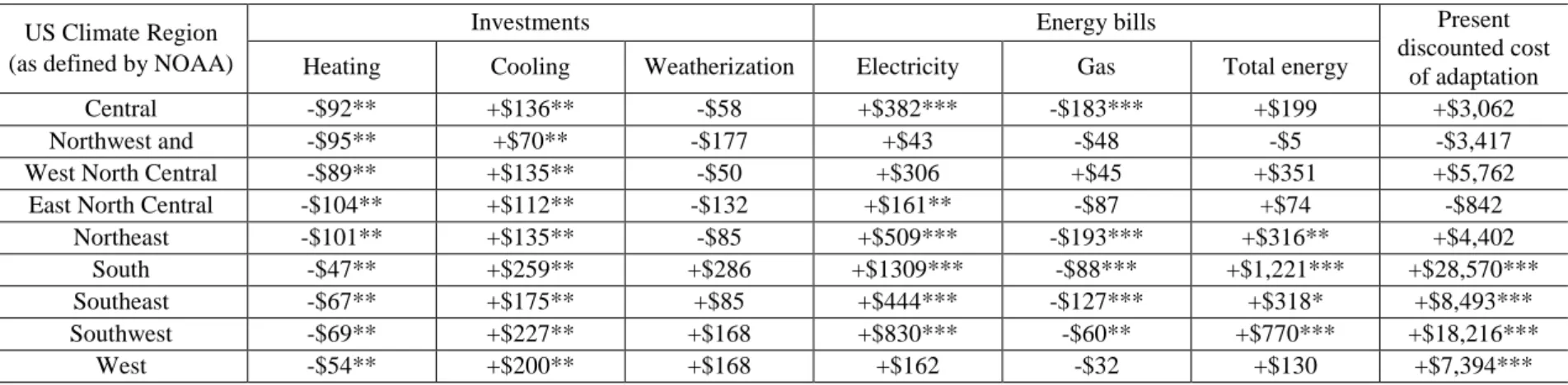
Our best estimate of the present discounted value of the cost for adapting to temperature increases under the A2 scenario is $5,600 per housing unit, accounting for both energy and investment costs. Even though the null hypothesis of a zero cost is rejected at 10%, this is still moderately low when we consider that the average price of a housing unit in our data is around 205,000 in real 2011 dollars: the cost of adaptation represents around 2.7% of the price of a US home. The reason is that the installation and more intensive use of additional air-conditioners are partially offset by reduced space heating needs. Consequently, we predict a major shift from gas, which is the main heating fuel, to electricity, which fuels air conditioners. Gas expenditure is expected to decrease by 25%, mostly in colder states, whereas electricity expenditure would increase by 29%, mostly in warmer states. Total residential energy expenditure would increase by 13% since electricity is sold at a higher price.
The empirical literature on adaptation in the residential sector is limited. The studies by Deschênes and Greenstone (2011) and Auffhammer and Aroonruengsawat (2011, 2012) are the most closely related to this paper. However, both papers only deal with intensive margin
5
adjustments3. Deschênes and Greenstone (2011) estimate that, by the end of this century, residential energy consumption could rise by 10-11% in the US as a result of climate change. Using a very large sample of monthly and geolocalized data, Auffhammer and Aroonruengsawat examine household-level electricity consumption data in California from 2003-2006. They find a modest 3-6% increase under the A2 scenario. Like us, all of these studies adopt a panel data approach with location-specific and time-fixed effects. Our simulations however produce higher energy cost estimates than those obtained by Auffhammer, Aroonruengsawat, Deschênes, and Greenstone because we account for energy-use changes that are induced by changes in the capital stock, and we predict a surge in air conditioning investments that mostly consume electricity. However, we do not evaluate household welfare. We only look at the monetary cost of adaptation, and ignore non-monetary benefits resulting from milder indoor temperatures (e.g. lower mortality, more comfort).4 If households make rational investment decisions, one might expect extensive margin adjustments to improve welfare.5
A few papers deal with the extensive margin, but with a more limited scope than ours. In a unified framework, Mansur et al. (2008) examine short-term energy consumption decisions and long-term fuel choices. Their (cross-sectional) analysis does not deal with the size of the investments associated with these decisions. Other studies focus on the diffusion of air conditioning. Davis and Gertler (2015) use microdata from Mexico to describe how electricity consumption increases with temperature given current levels of air conditioning, and how climate and income drive air conditioning adoption decisions. Like us, they predict a much larger increase in electricity consumption after incorporating the extensive margin; they do not provide any investment cost estimate. Rapson (2014) develops a structural model of demand for air conditioners, but does not focus on climate variables.
In the medium term, the margins of adaptation are constrained by the existing housing stock.6 More adaptation options are available if the time horizon is extended further: households can move into new dwellings that are more adapted to the new climatic regime (in particular,
3 See Auffhammer and Mansur (2014) for a recent review of the empirical literature on how climate impacts energy consumption.
4 Note that, in addition to energy consumption, Deschênes and Greenstone (2011) measure the welfare impacts associated with higher mortality.
5 The potential benefits of home adaptation can be huge, as illustrated by Barreca et al. (2016) who find that the progressive adoption of air conditioning throughout the 20th century explains 90% of the entire drop in the impact of excess heat on mortality in the US.
6 Constructing new buildings that integrate the new climatic conditions into their design can mitigate the problem (Kahn, 2010), but most adaptation in the next decades will involve existing dwellings.
6
because they are located in less exposed areas); firms develop new cooling and heating technologies; public authorities redesign urban spaces, etc. Neither this paper nor any of the studies mentioned above consider these longer-term adjustments. In this paper, we however discuss their implications for the cost estimate we provide. In general, the availability of additional strategies to adapt to climate change should reduce further the cost of climate change adaptation.
The remainder of this paper is structured as follows. The next section presents a conceptual framework and the equations that describe investment behavior and energy use. Section 3 describes the data and section 4 presents the estimation results. Section 5 assesses the magnitude of the estimates of the effect of climate change by simulating the A2 scenario.
2. Analytical framework
Figure 1 presents the framework that will be used throughout the paper. Temperature potentially affects energy use through two channels. First, it directly influences the quantity of energy used by installed energy-consuming durables (A in Fig. 1). The second is indirect: temperature modifies home occupiers' investment behavior and thus the housing capital stock (B), leading to further energy use adjustments (C). The paper primarily seeks to identify these causal links in order to evaluate the impact on investment and energy expenditures. To do so, we estimate two sets of equations, i.e. investment equations that relate the size of investments made in each period to temperature variations, and energy equations that relate the level of energy expenditures to temperature and to the stock of energy-related durables.
Figure 1: Causal relationships between temperature, energy consumption, and home capital stock
Temperature
Capital stock (e.g. insulation, AC,
heating equipment)
(A)
Energy consumption for heating and cooling: gas
and electricity
7
2.1. Investment equations
The dependent variable is the investment made in its dwelling by household i in period t (the data only describe homeowners). In order to limit potential aggregation biases, we consider specific categories of investment that are related to adaptation. The full panel of the AHS data (1985-2011) only makes it possible to identify two categories of adaptation-related home improvements: 1) the installation of major energy-consuming equipment, including major space-heating appliances and air conditioners (either room or central air conditioners); and 2) weatherization, (i.e. addition/replacement of foam, weather stripping and caulking) and, by extension, improvements to doors and windows, roofing and sidings that improve the energy integrity of dwellings7. The regressions will thus not produce specific results for investments in space heating and air conditioning. However, when performing the simulations in section 5, we introduce the assumption that investments in space heating and air conditioning are separable and strictly influenced by heating and cooling needs respectively to mitigate the problem.8
To identify the relationship between this variable and temperature variations, we fit the following linear equation:
𝐼𝑖ℎ𝑡 = 𝛼ℎ𝐶𝐷𝐷𝑖𝑡 + 𝛽ℎ𝐻𝐷𝐷𝑖𝑡+ 𝛾ℎ𝑋𝑖𝑡+ 𝜇𝑖ℎ+ 𝜏ℎ𝑡+ 𝜀𝑖ℎ𝑡 (1)
where 𝐼𝑖ℎ𝑡 denote the level of investment made by household 𝑖 in category ℎ (with ℎ = equipment, weatherization) and in period 𝑡. 𝛼ℎ, 𝛽ℎ, and 𝛾ℎ are (vector of) parameters to be estimated. The last term 𝜀𝑖ℎ𝑡 is the random error term.
𝐶𝐷𝐷𝑖𝑡 and 𝐻𝐷𝐷𝑖𝑡 capture the impact of temperature on investment. They are expected annual cooling degree days and annual heating degree days in year t and in the location of household i’s housing unit, respectively. These are standard measurements designed to reflect the demand for heating and for cooling. The precise definition of cooling degree days is the number of degrees a day's average temperature rises above 65° F, which is the temperature at which it is assumed that people start using air conditioning to cool their buildings.
7 Another less interesting category corresponds to all other indoor investments not directly related to climate change, i.e. changes to the bathroom; changes to the kitchen; home extensions; and other major indoor improvements. These are studied in Appendix K. As expected, we find no significant impact of temperature. 8 We also look at a shorter panel (1997-2011) in Appendix A, for which the distinction between investments in air conditioning and heating is possible. Results are less precise but qualitatively similar to those presented in the core of this paper.
8
Symmetrically, heating degree days are the number of degrees that a day’s average is below 65° F.
A crucial point is that 𝐶𝐷𝐷𝑖𝑡 and 𝐻𝐷𝐷𝑖𝑡 are expected degree days, not the contemporaneous values of these variables. The lifetime of investments in housing is relatively long so that the benefits from installing air conditioning or insulating in a house depend on future needs. Thus, if rational, households base their investment behavior on their expectations of future temperatures.
These expectations are however not observed in historical climate data. To solve this problem, we adopt an adaptive expectation framework. It assumes that households adjust their expectations based on some averaging of past climate values that are observed in the data.9 Consider the case of cooling degree days and let 𝑐𝑑𝑑𝑖𝑡 denote the contemporaneous number of cooling degree days that is actually observed in year t by household i. The adaptive model assumes the following relationship between expected degree days and observed (real) degree days:
𝐶𝐷𝐷𝑖𝑡 = 𝐶𝐷𝐷𝑖𝑡−1 + 𝜆(𝑐𝑑𝑑𝑖𝑡−1 − 𝑐𝑑𝑑𝑖𝑡 ) (2)
Eq. (2) means that the current expectation is composed of past expectations and an “error adjustment” term, which raises or lowers the expectations depending on the realized number of degree days.10 The parameter 𝜆 ∈ [0; 1] captures the adjustment speed between past and current expectations. When applying Eq. (2) recurrently over all past periods, expectations at time t of the CDD at t + 1 are equivalent to an exponentially weighted moving average:
𝐶𝐷𝐷𝑖𝑡 = 𝜆 ∑(1 − 𝜆)𝑘 𝑘=0
(𝑐𝑑𝑑𝑖𝑡−𝑘−1)𝑘+1 (3)
We use the same formula to calculate expected heating degree days. We estimate the value of 𝜆 by assuming that all households use a value that would make their predictions as accurate as possible. More specifically, we fit a non-linear regression based on Eq. (3).11 The estimated results are used to predict current values based on a weighted average of past values for all
9 Gelain and Lansing (2014) provide recent evidence that backward-looking expectations may operate on the housing market. They argue that such expectations are a better predictor of high volatility in price-rent ratios compared to rational expectations.
10 Note that this formula precisely gives the value of the cooling degree days in year t + 1 as expected in year t. We use the formula to calculate expectations in years t+1, t+2, t+3… Hence we implicitly assume that the household considers that the climate is stable during the investment lifetime.
11 This equation is slightly modified to account for the fact that we have a limited amount of lags in the model. We assume that since tends to one only when the number of lags tends to infinity for low values of .
9
households in our data. We then choose the 𝜆 that minimizes the prediction errors. The estimate is 𝜆 ≈ 0.30. This is equivalent to assuming that expectations mostly rely on the past 7-8 years.12
Using degree days may fail to account for potential nonlinearities in the marginal impact of temperature changes on investments. That is, it is assumed that a one-degree increase has the same effect on investment, whether it occurs on a mild day with temperatures of 70°F or during a 90°F heatwave. As a robustness check, we also estimate a more flexible specification including temperature bins, which gives estimates of the specific impact on investments at different temperature ranges (like in Deschênes and Greenstone, 2011). Results are not substantially different.
Let us now turn to the control variables included in vector 𝑋𝑖𝑡. The choice of adequate controls is complicated by the fact that climate potentially influences many variables. Take the example of household income. This is an obvious control candidate as it influences the propensity to invest. However, it is also reasonable to assume that temperature has an impact on its level. Recent empirical studies have actually confirmed this hypothesis (e.g., Dell et al. 2009). If this variable is included in 𝑋𝑖𝑡, the coefficients 𝛼ℎ and 𝛽ℎ will then not identify the full effect of climate, but only the direct effect of temperature, ignoring the indirect effect that passes through changes in income. This will then skew the results of our simulations.
To reduce this risk of "over-controlling", Dell et al. (2014) and Hsiang (2016) suggest excluding from the equation factors that are assumedly not influenced by temperature. Accordingly, in addition to income, we do not incorporate information on the investment prices because temperature probably influences local prices of energy-related investments: e.g. a higher demand for air conditioning induced by very hot summers will increase the local price of air-conditioners. In the same vein, we do not control for electricity and gas prices, even though they are clear determinants of the demand for heating and air conditioning equipment: temperature has direct impacts on energy production, transmission and distribution, and thus on energy prices. Finally, we also exclude the impact of past investments on current investments, because past investments depend on past expectations about climate. Hence, they are correlated with current weather shocks in a causal manner, provided that home occupiers form expectations with some rationality. Ultimately, we limit
12 We obtain similar results with a distributed lag model that includes three-year lags as control variables. Using current values provides results that are less precise. This assumes that households only consider contemporaneous heating degree days and cooling degree days when making long-term decisions (Appendix E).
10
ourselves to control the number of individuals living in the house, annual precipitation levels, and whether the neighborhood has a pipe gas supply.
The equation also includes time dummies (𝜏ℎ𝑡) and household-category fixed effects (𝜇𝑖ℎ). This means that we exploit location-specific time-varying variations of the temperature variables to predict the impact on investments. However, the coefficients 𝛼ℎ and 𝛽ℎ do not only identify the direct causal effect of a change in temperature on the demand for investments, but also the correlation between temperatures and investment levels, including income effects, and demand-side and supply-side effects. This assessment of temperature changes then yields a more complete measurement of their overall impact on investments. The negative side is that excluding these variables will limit the external validity of our results.
Note that household-category fixed effects control for residential sorting, a standard concern in this spatial setting. In our context, sorting is a form of adaptation: households that suffer less from intense heat are more likely to move into dwellings that are more exposed to heat, thereby reducing cooling energy and investment expenditures. The inclusion of household fixed effects leads us to ignore this role of relocation in adaptation.
Other issues
A common concern in the empirical literature is that investments are lumpy, with long periods of no investment (𝐼𝑖ℎ𝑡 = 0) interrupted by more active investment periods (e.g. Doms and Dunne, 1998). In our case, households may prefer to make all the necessary improvements at one point in time because of the hidden fixed costs. For example, home renovation limits the ability to live in a dwelling while it is being renovated.
Interpreting home improvements as a left-censored variable –investments are only observed when their value is positive– is a popular approach to deal with this problem. In Appendix F, we estimate two different latent variable models. The first is a panel tobit model with fixed effects based on Honore (1992). A weakness of this approach is to assume symmetric errors. To relax that assumption, we estimate the Wooldridge’s (2005) dynamic random effect panel tobit model, which specifies a functional form for the fixed effect. Another advantage is that the model accommodates persistent behavior. Results in Appendix F are very similar when it comes to the relative effect of heating and cooling degree days on investments. We however prefer the fixed-effect linear model, principally because it produces estimates of the fixed
11
effects, whereas Wooldridge’s approach requires additional controls to mimic a fixed-effect specification.13
Energy efficiency policies (e.g. tax credits or subsidized loans) that are implemented to influence investments in space heating, air cooling and weatherization in some states may create biases, as their existence is likely to be correlated with climate shocks. We simply exclude from the sample all observations in which households have benefited from energy efficiency subsidies (2% of the observations). As a robustness check, we use this piece of information to construct a dummy variable that is included in the equation. As this variable is likely to be endogenous – it reflects the existence of policies promoting energy efficiency at a local level14 – we use a control function approach. We observe only very slight differences in the results obtained by the two approaches (see Online Appendix H).
2.2. Energy expenditures
We separately estimate the demand for electricity and gas, which are the two main energy sources used in the US residential sector. Like Greenstone and Deschênes (2011) and Aufhammer and Aroonruengsawat (2011, 2012) we use a log-linear specification. The dependent variable is 𝐸𝑖𝑓𝑡, the logarithm of the annual energy expenditure in fuel f (with f = gas, electricity) of household i at time t:
ln(𝐸𝑖𝑓𝑡) = 𝜃𝑓𝑐𝑑𝑑𝑖𝑡 + 𝜆𝑓ℎ𝑑𝑑𝑖𝑡+ ∑ 𝜙ℎ𝑓𝐾𝑖ℎ𝑡 3
ℎ=1
+ 𝜔𝑓𝑌𝑖𝑡+ 𝜇𝑖𝑓+ 𝜏𝑓𝑡+ 𝜖𝑖𝑓𝑡 (4)
𝑐𝑑𝑑𝑖𝑡 and ℎ𝑑𝑑𝑖𝑡 are cooling degree days and heating degree days. Importantly, we use on-the-year values and not expectations, since energy consumption immediately reacts to temperature changes.
𝐾𝑖ℎ𝑡 measures the amount of capital in the housing unit in each investment category ℎ. As explained above, this is what distinguishes this paper from previous works on climate’s impact on residential energy use. 𝐾𝑖ℎ𝑡 roughly equals the sum of current and past investments
13 In addition, the model does not always converge due to the many dummy variables introduced to proxy a fixed-effect specification. It is common that dummy variables create convergence problems in random effect tobit models.
14 In particular, this variable only captures information about households that actually performed alterations. For the other households, we do not know whether they had access to government aid or not. In addition, this is a binary variable, whereas household choices are driven by the size of subsidies.
12
𝐼𝑖ℎ𝑡, 𝐼𝑖ℎ𝑡−1, 𝐼𝑖ℎ𝑡−2… that are discounted to account for obsolescence15. Its precise calculation is described in Appendix B. Note that, in addition to equipment and weatherization, we consider a third category including all other investments. The last category includes home improvements, like kitchen renovation, that could influence energy expenditure.
𝑌𝑖𝑡 is the vector of controls, which includes the log of family size, annual precipitation, and connection to pipe gas in the neighborhood. For the reasons discussed previously, we do not control for income and energy prices, as they are likely to be influenced by temperature. The equation includes a full set of household-by-fuel fixed effects, 𝜇𝑖𝑓, which absorb all household-specific time invariant household specificities. It also includes a set of time-by-fuel dummies, 𝜏𝑡𝑓, which, for instance, control for the general evolution of energy prices in the US that might affect energy expenditure. 𝜖𝑖𝑓𝑡 is an error term. Finally, 𝜆𝑓, 𝜙𝑓, θ𝑓, and 𝜔𝑓 are (vectors of) parameters to be estimated.
Sample selection
The fact that Eq. (4) is estimated separately for gas and electricity potentially generates a sample selection bias, as households choose the type of fuel used in their homes. This risk is however limited by the inclusion of household-by-fuel effects, which control for fuel selection prior to moving into the house. We also control for the availability of pipe gas, a major determinant of choosing gas over other fuel types. More generally, fuel switching occurs when installing new equipment and is thus infrequent: households report a change in main heating fuel concomitant to home equipment improvements in only 0.6% of observations in the data. Appendix T also presents a specification in which the dependent variable is the sum of electricity and gas expenditure levels. This is to consider that households jointly choose both expenditure levels. Results are similar to those obtained using separate equations.
Endogeneity of capital stocks
In Eq. (4), the different capital stocks variables are likely to be endogenous: they include the investments 𝐼𝑖ℎ𝑡 made in year t, which are simultaneously determined with 𝐸𝑖𝑓𝑡. As a result, any unobserved shock that affects investment is likely to be correlated with the error term.
One solution is to instrument for the stocks of capital in every category h with the lagged values of these stocks. The availability of these lags is very convenient to produce instruments
15 One difficulty is that investments are not observed before the year of purchase or construction. We estimate the stocks in that year relying on the sales price. All details are provided in Appendix B.
13
since the past capital stocks are not correlated with current shocks on energy expenditure. One difficulty, however, is that they are correlated with past shocks, implying that they are pre-determined. This precludes using a standard fixed effect IV model based on demeaning.
GMM estimators can circumvent this problem (Arellano and Bond 1991; Blundell and Bond, 1998). These are controversial tools when used to estimate dynamic panel data models where the dynamic component of the model is instrumented with its own lags.16 However, our concern is different – the choice of 𝐼𝑖ℎ𝑡 and the choice of 𝐸𝑖𝑓𝑡 are simultaneous – and we do not need a dynamic model. In our case, the exclusion restriction implies no correlation between the error term and the deeper lags of the capital stocks, which is weaker than assuming no correlation between the error term and the lagged dependent variable as requested in a dynamic model.
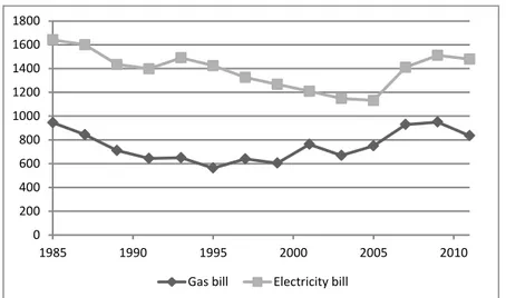
We use the system-GMM estimator, which offers high efficiency levels. This efficiency gain comes at the cost of an additional assumption compared to the alternative difference GMM model: the variables used in the model should be mean stationary. This seems a reasonable assumption in the case of residential gas and electricity demand in the US, since the real-time series of residential energy bills were not subject to trends or breaks during the sample period (see figure 2 below).17
Figure 2: Average energy bills in the sample used (in real 2011 dollars)
16 In this case, the exclusion restriction requires that the deeper lags of the dependent variable are not correlated with the contemporaneous error values. This is a strong assumption in many real situations.
17 We cannot formally test for mean stationarity using unit root tests since our panel is not balanced.
0 200 400 600 800 1000 1200 1400 1600 1800 1985 1990 1995 2000 2005 2010 Gas bill Electricity bill
14
System GMM can be calibrated in a series of ways. Our baseline specification uses the first-differenced third lags of the capital stock as instruments. We use first differences, and not orthogonal deviations, because the data does not include many gaps. We make multiple robustness checks to ensure that the results do not depend on these two choices.18
3. Data
We rely on three main data sources: the American Housing Survey for data on housing units, home improvements, energy consumptions and household characteristics; the Global Historical Climatology Network (GHCN) Daily for meteorological data; and the ECHAM model for climate change predictions. This section briefly describes the data sources and reports summary statistics.
3.1. Data sources
AHS data
The data on housing units, home improvements, energy expenditures and households are taken from the national sample of the American Housing Survey, which covers Metropolitan Statistical Areas (MSAs). We use longitudinal data from 14 waves of the national AHS from 1985 to 2011.19 The housing units are located in the 128 MSAs with more than 100,000 inhabitants. These MSAs are spread all over the United States, and experience very different climatic conditions. Note also that the sample only includes owner-occupied units for which information on renovation investments is available.
The AHS includes information on nine different types of home improvement. The weatherization variable is constructed by adding together investments made in the following four categories: roofing; insulation; sidings; and storm doors and windows. The equipment variable is identified as a single category in the survey, precluding, as mentioned above, the distinction between investments in air conditioning and space heating.20 Nevertheless, households report their main heating fuel and their main fuel for air conditioning. This
18 We provide results of models using orthogonal deviations (Appendix N), the 4th lags of the capital stock as instruments (Appendix O), and the difference GMM estimator (Appendix P). We also estimate a model where we have excluded all of the endogenous capital variables (Appendix Q) and a dynamic panel data model (Appendix S).
19 Waves prior to 1985 cannot be used in a panel data analysis because the AHS was redesigned in 1985 and the units surveyed before and after 1985 are different.
20 In 1997, the typology was refined, but we had to stick to the previous typology to be able to use the entire study sample from 1985. We perform robustness checks on the reduced panel of 1997-2011 in Appendix A. Results are imprecise due to the halving of the sample, but consistent with those obtained with the full panel.
15
information is used in some specifications to construct interaction variables used to proxy the specific impact of investments in heating and cooling equipment (more detail in subsection 5.1).
For each type of home improvement, we observe the level of biannual investments between 1985 and 2011. However, the value of the stock of capital already embodied in a home before 1985 is unobserved, which is vital for constructing the capital stock variables included in energy equations. We derive this initial stock – and from this the value of 𝐾𝑖ℎ𝑡 – from the purchase price or the construction cost of the housing units as registered in the American Housing Survey after a transaction, or after construction for new buildings. Appendix B precisely presents the method.
The AHS also provides information on home occupiers. In particular, it identifies when a household left a given housing unit and when new occupiers moved in. This information is used to construct household-specific fixed effects. Information on the level of energy expenditure, on whether the neighborhood has access to pipe gas, and commuting times (this variable is used as an instrument in Appendix S) is also extracted from the AHS.
Information on the precise location of each housing unit – a decisive variable to relate each unit to local climatic conditions – is not available for all areas. We thus take the centroid of the MSA as a proxy. This choice is likely to generate limited biases since temperature anomalies do not vary much within a given MSA.
Weather data
The weather data are taken from the Global Historical Climatology Network (GHCN) Daily. We extracted land-based (in situ) historical observations recorded from 1970 to 2011 by 22,000 meteorological stations that match the MSAs included in our sample and that operate at least a certain number of days during a year. More specifically, we only selected stations located within a 50km radius of the centroid of an MSA and that record daily information for at least 20 days each month of the year, and calculated averages for each MSA.
The key variables are the annual heating degree days, cooling degree days, and annual precipitations in millimeters. We estimate alternative specifications using the number of days that fall within 10°F temperature bins (the first bin is “below 10°F” and the last one “above 90°F”). We also look at nonlinearities in the impact of days with precipitations. We use as variables the number of days without precipitation, and the number of days with precipitations between 1-50mm, 50-100mm, 100-200mm and above 200mm.
16
Climate change prediction data
State-level monthly average temperature predictions are drawn from the 5th version of ECHAM, an atmospheric general circulation model developed at the Max Planck Institute for Meteorology. To ease comparability with other studies, we focus on the “business-as-usual” A2 scenario and its predictions for the end of the century (2080-2099). A2 is a scenario in which a relatively high amount of GHG emissions is released into the atmosphere, leading to a global average surface warming of 6.1°F in 2090-2099 relative to 1980-1999 (IPCC, 2007).
US state-specific averages are accessible using the US Geological Survey’s Regional Climate Change Viewer (RCCV). The RCCV uses a downscaling method of the output of ECHAM, averages temperatures within states, and then compares the historical period of 1980-1999 with the ECHAM model’s output for 2080-2099. This gives a predicted daily mean temperature increase for each month and state. This increase is added to all the days of the historic weather data to compute daily average temperature forecasts for 2080-2099. We then use these daily temperature forecasts to predict state-level changes in heating degree days and cooling degree days.
3.2. Summary statistics
Investment, energy expenditure, and household data
Table 1 provides descriptive statistics for the AHS data used as a basis for model estimations. The sample is composed of a panel of 58,887 observations21. This includes 10,522 housing units and 24,680 households. The investment frequency is low (7.1% for the installation of equipment and 19.0% for weatherization), but the average investment size is significant (around $3,700). This lumpiness could justify the use of a latent variable model; Appendix F presents tobit results that are however similar to those of the base linear model. Note that adaptation-related investments do not constitute the biggest share of renovation expenditures. In particular, the capitalized investment in equipment is minor compared to the other categories.
Weather and Climate Change Statistics
Detailed weather statistics for the entire sample and by US climatic region are provided in Table 2. We report information on daily temperature, number of heating and cooling degree
21 This is far fewer than the 262,872 observations of geographically located and owner-occupied units between 1985 and 2011. However, many values are missing, in particular the values of the purchase price or construction cost. Outliers have also been excluded (see more details in Appendix C).
17
days, and number of days below 10°F and above 90°F. Using the same format, Panel B presents the impacts of climate change based on the ECHAM model and for the A2 scenario. These figures show high heterogeneity between regions in terms of daily temperature, but also of the number of days with extreme temperature (cold or hot). The US is obviously not representative of the climatic conditions observed all over the world, but it nevertheless provides a significantly diversified sample.
Table 1: Descriptive statistics of AHS data
Variable Unit Mean Std. deviation
Investments in equipment
Capitalized investments $ 9,902 6,628
Respondents declaring an investment % 7.1 -
Expenditure if an investment is made $ 3,699 2,701
Investments in weatherization
Capitalized investments $ 52,660 35,614
Respondents declaring an investment % 19.0 -
Expenditure if an investment is made $ 3,792 4,369
Investments in other indoor amenities
Capitalized investments $ 100,188 67,374
Respondents declaring an investment % 32.6
Expenditure if an investment is made $ 5,043 9,046
Energy expenditure and consumption
Annual electricity expenditure $ 1,304 745
Annual gas expenditure $ 684 656
Annual electricity consumption MM.btu/year 36.9 22.8
Annual gas consumption MM.btu/year 59.7 57.6
Other relevant variables
Number of people in household # 2.76 1.51
Housing units connected to pipe gas % 76.1 -
Commuting time min. 21.0 17.5
Square footage of unit sq. ft. 2,130 1,266
House price at time of purchase $ 206,042 157,562
Notes: Source: AHS. Survey years: 1985-2011. Max. number of observations: 58,874. Comments: all the variables in dollars are expressed in 2011 real dollars. The correction of nominal values was made using the US Consumer Price Index of the Bureau of Statistics of the US Department of Labor.
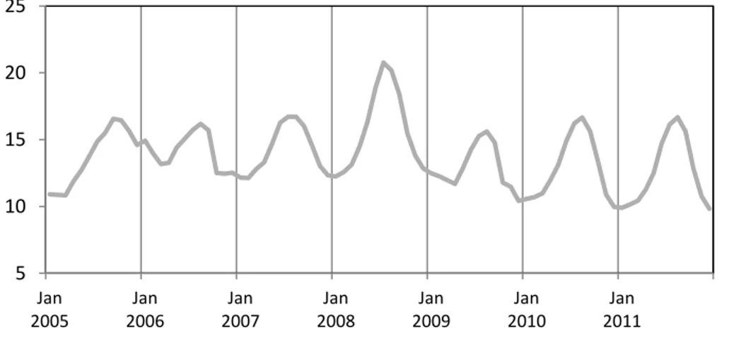
Figure 3 shows the average number of days falling within a given temperature bin. The grey bars report the averages as observed with the GHCN data of NOAA over the 1985-2011 period and the black bars report the averages as predicted by ECHAM under the A2 scenario. The A2 scenario predicts a dramatic increase in hot days (80-90°F) and very hot days (>90°F) in 2090-2099, mostly in hot regions. In contrast, the number of days below 70°F decreases uniformly across the different temperature bins.
18
Table 2: Summary statistics of climate data
Annual averages Daily temperature
Heating degree days
Cooling degree
days Days <10°F Days > 90°F Panel A. Historical temperature data (1985-2011)
All housing units 55.7 4,534 1,128 2.6 2.4
Cold regions 50.8 5,871 681 4.1 0.0
Central 51.9 5,732 959 4.7 0.0
Northwest 49.6 5,730 116 0.1 0.0
West North Central 50.3 6,357 1,005 11.7 0.0
East North Central 47.5 7,061 666 13.1 0.0
Northeast 52.7 5,397 907 1.3 0.1 Hot regions 63.2 2,474 1,799 0.2 6.2 South 65.6 2,319 2,552 0.3 2.3 Southeast 60.6 3,238 1,635 0.1 0.0 Southwest 62.6 3,289 2,430 1.1 31.3 West 62.9 1,972 1,223 0.0 3.1
Panel B. Predicted change from ECHAM model under the A2 scenario (2080-2099)
All housing units +7.4 -1,529 +1,168 -1.8 +12.9
Cold regions +7.4 -1,834 +869 -2.8 +2.4
Central +7.6 -1,736 +1,029 -3.5 +4.1
Northwest +6.3 -1,787 +527 -0.1 0.0
West North Central +7.4 -1,684 +1,026 -6.4 +6.9
East North Central +7.7 -1,951 +850 -8.2 +1.5
Northeast +8.0 -1,891 +1,021 -1.1 +3.2 Hot regions +7.4 -1,064 +1,620 -0.2 +28.9 South +7.8 -889 +1,959 -0.2 +68.2 Southeast +7.1 -1,264 +1,327 0.0 +8.7 Southwest +8.2 -1,290 +1,721 -0.7 +38.8 West +6.9 -1,008 +1,514 0.0 +11.3
Notes: The climate variables are averaged over all of the observations of the AHS datasets used in the regressions and the simulation. Hence, regional averages are not representative of the regions, but of the sample of housing units within each region. When a unit is located in a metropolitan area that overlaps two or three states, it enters the calculation of the averages in all of the states it overlaps, but with a weight of 1/2 or 1/3.
19
Figure 3: Observed and forecasted number of days falling within each temperature bin
Notes: Figure 3 shows the historical average and the predicted average in the distribution of daily mean temperatures across ten temperature-day bins. The “Observed in dataset” bars represent the average number of days per year in each temperature category for the all of the observations in the sample, covering the period 1985-2011. The “Forecasted” bars represent the average number of days per year in each temperature category based on the output of the ECHAM model under the A2 scenario and for the period 2080-2099, and for all of the observations of the sample used in the simulation.
4. Results
This section is divided into two subsections. The first provides estimates of the relationship between temperature and capital investments, and the second examines the impact of temperature and investment on energy expenditure.
4.1. Adaptation investments
The base results for investments in equipment and weatherization are displayed in Table 3. In Appendices E-J, most of the hypotheses used to calibrate the models are tested in a series of robustness checks that confirm our findings (using contemporaneous or lagged degree days, estimating left-censored models, excluding investments made before leaving the house, including observations for which an energy efficiency subsidy was granted, including regional trends or interactions between time and degree days).
We find a statistically significant impact of expected heating and cooling degree days on investments in equipment. The two coefficients are positive, consistent with the hypothesis that households purchase more (or larger) heaters when winter temperatures fall and more air conditioners when summer temperatures increase. The impact of heating and cooling degree
0 10 20 30 40 50 60 70 80 <10 10-20 20-30 30-40 40-50 50-60 60-70 70-80 80-90 >90 Temperature bins (°F)
20
days on weatherization is also positive and significant. Note that precipitation has no significant impact. As a robustness check, we show in Appendix K that investments in other indoor amenities (changes to the bathroom; changes to the kitchen; home extensions; and other major indoor improvements) are not sensitive to changes in expected heating and cooling degree days, confirming the specificity of investments in equipment and weatherization.
Table 3: Main results for investments in energy-related home improvements
Type of investment Equipment Weatherization
Expected heating degree days 0.106 0.328
(0.0501) (0.153)
Expected cooling degree days 0.264 0.441
(0.114) (0.223)
Expected precipitations -0.00159 0.0291
(0.00738) (0.0206)
No. people in unit 6.039 23.31
(9.809) (19.46)
Connection to pipe gas 225.0 245.5
(61.07) (88.33)
Observations 42,221 42,010
Notes: standard errors (clustered at household level) in parentheses. Models include household fixed effects and time-dummies. Constant terms are not reported.Standard errors are clustered at household level.
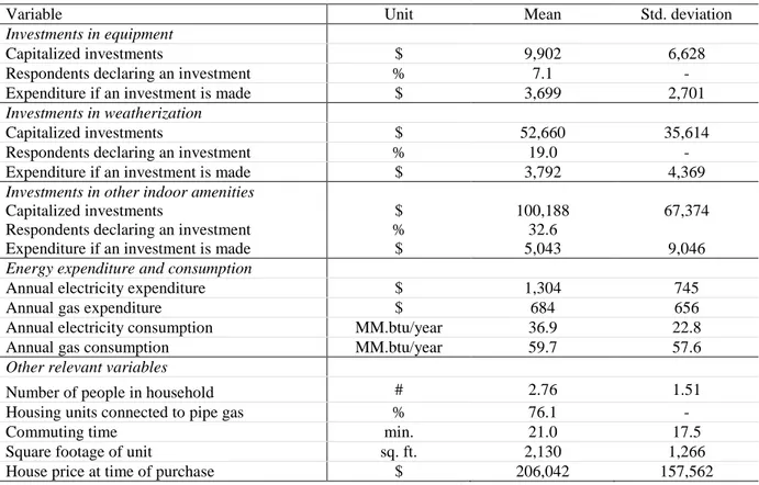
Table 4 displays the results of alternative models using temperature bins. The existence of nonlinearities in the relationships between degree days and investments is confirmed. The impact at the extremes is stronger than that observed in the comfort zone of 60-70°F22. We also find a local investment maximum at 30-40°F, when it starts freezing and snowing.
22 Note that the coefficients for the coldest bin are not statistically significant, probably due to too few observations.
21
Table 4: Linear investment models using temperature bins
Type of investment Equipment Weatherization
Expected # days with temperature:
Below 10°F 1.349 8.333 (5.788) (13.10) Between 10-20°F 10.78 21.75 (5.130) (10.77) Between 20-30°F -5.469 7.710 (3.722) (8.040) Between 30-40°F 3.687 10.90 (1.915) (6.149) Between 40-50°F 2.437 7.812 (2.349) (5.302) Between 50-60°F 2.810 7.938 (2.032) (4.343) Between 60-70°F - - Between 70-80°F 2.343 4.618 (1.791) (3.813) Between 80-90°F 4.414 9.424 (2.531) (4.888) Above 90°F 14.03 23.62 (6.661) (9.806)
Expected days with precipitations:
No precipitation - - Between 0-50mm 1.017 2.033 (0.893) (1.823) Between 50-100mm -5.467 -3.430 (3.017) (5.723) Between 100-200mm 2.043 6.030 (3.103) (6.022) Above 200mm -0.328 9.834 (3.537) (9.460)
No. people in unit 6.094 23.42
(9.806) (19.45)
Connection to pipe gas 225.3 246.4
(60.97) (88.38)
Observations 42,221 42,010
Notes: standard errors (clustered at household level) in parentheses. Models include household fixed effects and time-dummies. Standard errors are clustered at household level.
4.2. Energy expenditure
Table 5 displays results for gas and electricity expenditure. For each fuel type, we estimate the base model described by Eq. (4) and a variant where we use interactions of the equipment capital with the fuel used to heat and cool the house. Columns (1) and (3) thus provide estimates of the average impact of a change in equipment on energy demand across all households and years, while this impact can differ according to the main heating and the main cooling fuel declared by households in columns (2) and (4). The nature of the fuel gives an
22
indication of the type of equipment installed in the housing unit. We will use the results obtained with these models when running simulations in the next section in order to deal with the problem that we cannot distinguish between investments in heating or cooling in the data.
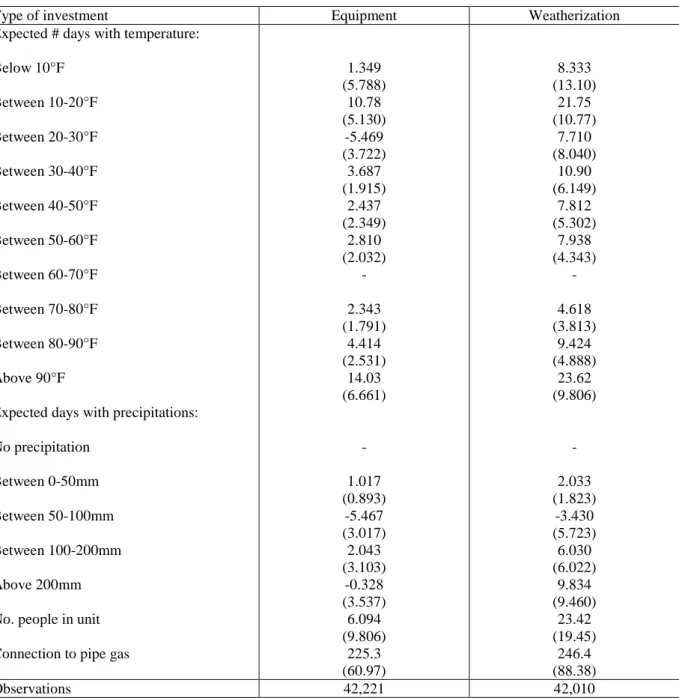
In the base specifications (1) and (3), households use more gas and electricity when the number of heating degree days increases as expected. It is also intuitive that cooling degree days increase electricity expenditure as most homes are equipped with electric air conditioners. In contrast, the significant and positive impact of cooling degree days on gas expenditure is more surprising, as gas is rarely used for cooling (around 3% of the households in the sample). Its interpretation highlights the fact that changes in energy prices are also a channel through which climate change affects adaptation expenditures: In the US, natural gas usage has two seasonal peaks. The first peak occurs during the winter, when cold weather increases the demand for natural gas space heating in the residential and commercial sectors. A second peak occurs in the summer when air conditioning use pushes up demand for electric power, an increasing portion of which is provided by natural gas-fired generators. Surprisingly enough, and for reasons related to gas storage technologies, gas prices only peak in summer months. The seasonal variation is high: during the study period (1985-2011), the annual maximum price of natural gas delivered to residential consumers, generally observed either in July or August, was on average 45% higher than the minimum price observed in December or January.23 Figure 4 illustrates this pattern by plotting the evolution of residential gas prices between January 2005 and December 2011. Coming back to the results of model (4), gas expenditure increases with cooling degree days because households continue to use gas in summer months to fuel water heaters, stoves, dryers, and other equipment so that the summer price peak significantly inflates their gas bill. The global warming expected in the future would reinforce this effect: by increasing the electricity consumption of air conditioners, higher summer temperatures would boost gas consumption by electric power generators, and push up gas prices in summer months.
23
Table 5: System GMM estimation of energy expenditure models
Dependent variable Ln. Electricity Expenditure Ln. Gas Expenditure
(1) (2) (3) (4)
Heating degree days 0.0137 0.00808 0.142 0.139
(0.00462) (0.00565) (0.00570) (0.00586)
Cooling degree days 0.176 0.129 0.0868 0.0856
(0.0110) (0.0209) (0.0144) (0.0144)
Capital in equipment 0.0131 0.00385
(0.00507) (0.00619)
x heating fuel is electricity 0.0176 (0.0119) x AC fuel is electricity 0.0203
(0.00778)
x heating fuel is gas 0.0184
(0.00925)
x AC fuel is gas 0.00104
(0.0191) Capital in weatherization -0.00360 -0.00287 -0.00219 -0.00291 (0.00173) (0.00171) (0.00210) (0.00211) Capital in other amenities 0.00141 0.00128 0.00218 0.00122
(0.000887) (0.000889) (0.00107) (0.00109)
Precipitations 0.0139 0.0146 0.0154 0.0161
(0.000771) (0.000784) (0.000997) (0.00105)
No. people in unit 0.0852 0.0852 0.0433 0.0444
(0.00220) (0.00218) (0.00242) (0.00244)
Connection to pipe gas -0.173 -0.0925 0.193 0.160
(0.00856) (0.0556) (0.0376) (0.0406)
Observations 50,000 50,000 37,244 37,244
Hansen test 0.12 0.36 0.09 0.16
Number of instruments 85 107 85 107
Notes: standard errors (clustered at household level) in parentheses. Models include household fixed effects and time-dummies. Constant terms are not reported. Capital variables are instrumented using third lags. Interactions are instrumented using third lag of capital in equipment times a dummy variable that takes the value of one if main heating/cooling fuel is different from gas or electricity. This is to avoid instruments to be correlated with changes in fuel choice. For heating degree days, cooling degree days, precipitations and all the capital variables, the reported coefficients have been rescaled since the model is log-linear. They correspond to a marginal change in the log of the dependent variable when the independent variables increase by 1000.
Figure 4: US price of natural gas delivered to residential consumers from Jan 2005 to Dec 2011 (in dollars per cubic feet)
Source: US Energy Information Administration (http://www.eia.gov) 5 10 15 20 25 Jan 2005 Jan 2006 Jan 2007 Jan 2008 Jan 2009 Jan 2010 Jan 2011
24
Turning next to the capital variables, all of the results are in line with expectations. The stock of equipment appears to have a positive impact on electricity expenditures in model (1). When the variable is interacted in model (2), results show that the positive effect is in fact only recorded when electricity is used for air conditioning. In columns (3) and (4), we find that investment in equipment increases gas expenditure when gas is used as the main heating fuel.
Weatherization also tends to reduce energy expenditures, but this negative impact is only statistically significant for electricity. Note also that capital in other amenities is positively correlated with gas and electricity use, which indicates that some of these investments increase heating and cooling needs, e.g. in the case of home extensions. The coefficients of the control variables show the expected signs, i.e. family size drives expenditure upwards and connection to pipe gas encourages households to choose gas heating.
Similar results are obtained when the specification is slightly changed. Appendix M gives results with alternative climate variables. In Appendix U, we estimate a model of energy consumption instead of energy expenditure and control for electricity and gas prices, where prices are instrumented using pre-sample information. The magnitude and statistical significance of the coefficients are very similar.
5. Impacts of climate change
This section aims to exploit the empirical results of investment and energy expenditure to estimate the impact of higher temperatures on energy expenditure and the resulting adaptation cost. The predictions are calibrated for the A2 scenario of IPCC and they rely on the ECHAM model of the Max Plank Institute, as described in section 3.
5.1. Simulation methodology
We proceed in three steps. First, we use the estimated coefficients of the fixed-effect investment models to compute the impact of a change in expected heating or cooling degree days on the average amount of equipment and the weatherization level in the housing unit. Second, we use the output of the panel models of energy expenditure to derive energy expenditure estimates that account for potential adjustments in capital calculated in the first step. Third, we calculate the cost of adaptation by adding up the variations of capital and
25
energy expenditures induced by the shift from the situation observed during the study period to the A2 scenario.24 We describe these steps in turn.
Step 1: Predicting investments
The first step involves no particular challenge. The estimated impact of predicted temperature changes in equipment investments in a given housing unit and year is calculated as follows:
∆𝐼𝑖𝑒𝑡 = 𝛼̂𝑒∆𝐻𝐷𝐷𝑖𝑡+ 𝛽̂𝑒∆𝐶𝐷𝐷𝑖𝑡
That is, the predicted change in heating and cooling degree days ∆𝐻𝐷𝐷𝑖𝑡 and ∆𝐶𝐷𝐷𝑖𝑡 is multiplied by the corresponding impact on investment (𝛼̂𝑒 and 𝛽̂𝑒).
Step 2: Predicting energy expenditure
The second step is more challenging and requires a number of assumptions. The first problem is that Eq. (4) does not distinguish between investments in cooling and heating equipment and thus relies on the simplifying assumption that purchasing cooling or heating equipment has the same impact on energy expenditure. Denoting 𝐾𝑖𝑡𝑐𝑜𝑜𝑙𝑖𝑛𝑔 and 𝐾𝑖𝑡ℎ𝑒𝑎𝑡𝑖𝑛𝑔 as the respective stock of cooling and heating equipment, this formally translates into:
𝜕 ln(𝐸𝑖𝑓𝑡) 𝜕𝐾𝑖𝑡𝑐𝑜𝑜𝑙𝑖𝑛𝑔 =
𝜕 ln(𝐸𝑖𝑓𝑡)
𝜕𝐾𝑖𝑡ℎ𝑒𝑎𝑡𝑖𝑛𝑔 = 𝜙𝑒𝑓
This restriction is problematic as temperature increases typically modify the composition of the equipment stock: home occupiers purchase more cooling equipment while reducing their stock of heating equipment.
To circumvent the problem, we proceed as follows. We first use the investment equation to predict investments in the two categories of equipment by assuming that, if a change in heating degree days increases the amount of capital invested, this corresponds to an increase in the level of investments in heating equipment. Formally, the estimated impact of predicted temperature changes on heating equipment investments in a given housing unit and year is:
∆𝐼𝑖𝑡ℎ𝑒𝑎𝑡𝑖𝑛𝑔= 𝛼̂𝑒∆𝐻𝐷𝐷𝑖𝑡
24 The simulation of the impacts of climate change was obtained employing econometric models that use heating and cooling degree days as the main variables of interest. Alternatively, we could have used models with temperature bins. Point estimates are similar when doing so for the entire sample, although confidence intervals widen because the effects of some temperature bins are imprecisely estimated. The use of heating and cooling degree days constrains the model to make linear extrapolations of the effect that these extreme days have on energy demand. This actually leads to more reliable results.
26
Symmetrically, if a change in cooling degree days increases the amount of capital invested, this corresponds to the purchase of cooling equipment so that ∆𝐼𝑖𝑡𝑐𝑜𝑜𝑙𝑖𝑛𝑔 = 𝛽̂𝑒∆𝐶𝐷𝐷𝑖𝑡.
The investment models predict the annual flows of investments while we need the capital stocks to use the energy expenditure model. We derive the value of ∆𝐾𝑖𝑡𝑐𝑜𝑜𝑙𝑖𝑛𝑔 and ∆𝐾𝑖𝑡ℎ𝑒𝑎𝑡𝑖𝑛𝑔 by assuming that these variations equal the predicted variations of annual investments divided by the depreciation rate of capital. This is equivalent to assuming that the same investment has been made in all previous periods. This assumption is not heroic as we make long-term predictions in which home occupiers have plenty of time to adjust their capital stocks. We set the depreciation rate of capital to 2%, which corresponds to the depreciation rate of real estate as estimated by Harding et al. (2007) based on AHS data
Then we infer the marginal impacts of ∆𝐾𝑖𝑡𝑐𝑜𝑜𝑙𝑖𝑛𝑔 and ∆𝐾𝑖𝑡ℎ𝑒𝑎𝑡𝑖𝑛𝑔 from the results of models (2) and (4) where the equipment capital is interacted with binary variables indicating the fuel used. In these models, the estimated marginal impact of the equipment capital is:
𝜕 ln(𝐸𝑖𝑓𝑡)
𝜕𝐾𝑖𝑒𝑡 = (𝜙𝑓1∙ 𝑎𝑓𝑡) + (𝜙𝑓2∙ 𝑏𝑓𝑡) (5)
where 𝑎𝑓𝑡 and 𝑏𝑓𝑡 indicate whether the fuel used for heating and cooling is 𝑓, respectively. This equation assumes that any equipment that uses a fuel other than 𝑓 has no impact on the expenditure for 𝑓: 𝜕𝑙𝑛(𝐸𝑖𝑓𝑡) 𝜕𝐾⁄ 𝑖𝑒𝑡 = 0 if 𝑎𝑓𝑡 = 𝑏𝑓𝑡 = 0.
Consider now the case where the fuel 𝑓 is only used for heating (𝑎𝑓𝑡 = 1 and 𝑏𝑓𝑡 = 0). It sounds reasonable to assume that any impact of 𝐾𝑖𝑒𝑡 on the consumption of fuel 𝑓 is exclusively due to an adjustment of the heating equipment stock. Formally, this writes:
𝜕 ln(𝐸𝑖𝑓𝑡) 𝜕𝐾𝑖𝑒𝑡 = 𝜕 ln(𝐸𝑖𝑓𝑡) 𝜕𝐾𝑖𝑡ℎ𝑒𝑎𝑡𝑖𝑛𝑔= 𝜙𝑓1 if 𝑎𝑓𝑡 = 1 and 𝑏𝑓𝑡 = 0 Symmetrically, we have 𝜕 ln(𝐸𝑖𝑓𝑡) 𝜕𝐾𝑖𝑒𝑡 = 𝜕 ln(𝐸𝑖𝑓𝑡) 𝜕𝐾𝑖𝑡ℎ𝑒𝑎𝑡𝑖𝑛𝑔= 𝜙𝑓2 if 𝑎𝑓𝑡 = 0 and 𝑏𝑓𝑡 = 1
Last, if we further assume no complementarities between heating and cooling investments, the marginal impacts of 𝐾𝑖𝑡𝑐𝑜𝑜𝑙𝑖𝑛𝑔 and 𝐾𝑖𝑡ℎ𝑒𝑎𝑡𝑖𝑛𝑔 continue to be equal to 𝜙𝑓1 and 𝜙𝑓2 in the case